


1. Introduction
There have been extensive studies on understanding swimming and locomotion of biological swimmers (e.g. bacteria and microalgae) in microfluidic environments where inertia is negligible (Purcell Reference Purcell1977; Lauga & Powers Reference Lauga and Powers2009). Especially, the recent advancements in nanotechnology and fabrication permit biomimetic medical micro-/nano-robots to navigate in non-Newtonian synthetic or biological fluids (Nelson, Kaliakatsos & Abbott Reference Nelson, Kaliakatsos and Abbott2010; Li et al. Reference Li, de Ávila, Gao, Zhang and Wang2017; Palagi & Fischer Reference Palagi and Fischer2018; Wu et al. Reference Wu, Chen, Mukasa, Pak and Gao2020). Understanding the microscale locomotion dynamics in complex anisotropic fluids is essential to design such microrobots that can efficiently operate inside the body for clinical applications. Of particular interest here is to uncover the propulsion mechanism of undulatory microswimmers in a class of anisotropic fluids, such as liquid-crystalline polymers, with orientation-dependent physical and material properties. For example, experimental observations have suggested that, when placed in solutions of liquid-crystal (LC) molecules (chromonic liquid-crystal disodium cromoglycate), swimming bacteria may exhibit intriguing behaviours, such as nematic director guided moving trajectories and activity-triggered topological defect dynamics, due to the coupling between the flow generation and the orientational order of the liquid medium (Zhou et al. Reference Zhou, Sokolov, Lavrentovich and Aranson2014; Lavrentovich Reference Lavrentovich2016; Zhou Reference Zhou2018).
Nevertheless, compared with the large body of literature on understanding the dynamics in isotropic Newtonian or non-Newtonian fluids, so far there have been only a minimal number of theoretical and computational models developed to understand swimming and locomotion in anisotropic fluids (Lintuvuori, Würger & Stratford Reference Lintuvuori, Würger and Stratford2017; Zhou et al. Reference Zhou, Tovkach, Golovaty, Sokolov, Aranson and Lavrentovich2017; Cupples, Dyson & Smith Reference Cupples, Dyson and Smith2018; Daddi-Moussa-Ider & Menzel Reference Daddi-Moussa-Ider and Menzel2018; Holloway et al. Reference Holloway, Cupples, Smith, Green, Clarke and Dyson2018; Rajabi et al. Reference Rajabi, Baza, Turiv and Lavrentovich2021). Most of these studies treat the fluid phase as suspensions composed of small LC molecules, and the corresponding mathematical descriptions of the constitutive relations are often built upon the classical LC models of Ericksen–Leslie (EL) or Landau–de Gennes type that use phenomenological energy functions to characterize the bend, twist and splay deformations for the LC's orientational topological structures (DeGennes Reference DeGennes1974; Larson Reference Larson1999). Also, undulatory microswimmers are modelled as either a rigid rod-like particle (Zhou et al. Reference Zhou, Tovkach, Golovaty, Sokolov, Aranson and Lavrentovich2017) or infinitely long swimming sheets (Krieger, Spagnolie & Powers Reference Krieger, Spagnolie and Powers2015, Reference Krieger, Spagnolie and Powers2019). Recently, Lin, Chen & Gao (Reference Lin, Chen and Gao2021) developed a fluid–structure interaction model to study the anisotropic undulatory swimming motion of a finite-length flexible swimmer in a LC fluid for the first time. Instead of using similar phenomenological, top–down LC models, we adopted a bottom–up  $Q$-tensor model coarse-grained form of Doi's kinetic theory (Doi & Edwards Reference Doi and Edwards1988) to describe the ambient fluid as suspensions of long, stiff liquid-crystalline polymers. Combining asymptotic analysis and direct simulations, we have studied and illustrated the enhanced (retarded) swimming motions in the nematic regime when the swimming direction is parallel with (perpendicular to) the nematic director.
Using the same  $Q$-tensor model of the Doi type, we extend the studies of simple parallel or perpendicular gaits to more general scenarios when the swimming direction is initially misaligned with the director. This work is also inspired by the analytical model by Shi & Powers (Reference Shi and Powers2017), who obtained the asymptotic solutions of a Taylor swimming sheet in solutions of small LC molecules with an arbitrary alignment angle. Moreover, they demonstrated that the misalignment between the swimming sheet and the director field could effectively produce a net body torque via the imposed anchoring condition of the director field on the wavy body. It is natural to ask (i) whether the misalignment condition will similarly lead to net polymer torque when using Doi's
  $Q$-tensor that does not require any anchoring condition to enforce alignment, and (ii) how a finite-length swimmer responds to such torque-imbalanced conditions arising from the LCP phase. Seeking the answers to these questions will provide quantitative understandings of both efficiency and stability of undulatory gaits of microswimmers, either biological or man-made, when navigating in anisotropic fluids.
The paper is organized as follows. Section 2 revisits the mathematical formulation of the fluid–structure interaction framework by Lin et al. (Reference Lin, Chen and Gao2021). In § 3, we perform the asymptotic solutions of Taylor's swimming sheet, and carry out numerical simulations for infinitely long sheets and finite-length swimmers using the immersed boundary (IB) method. Finally, we conclude and make some discussions in § 4. A few benchmarks studies and the derivation of the asymptotic solutions are presented in the appendices.
2. Mathematical model
We first set up the problem and review the dimensionless equations of the mathematical model developed by Lin et al. (Reference Lin, Chen and Gao2021) for completeness. Consider a one-dimensional flexible swimmer of length  $L_s$, whose undulatory kinematics can be described by the parametric form
  $\boldsymbol {X}(s,t)$ in terms of the local arc length
  $s\in [0,L_s]$ and time
  $t\geqslant 0$. The swimmer is initially positioned along the
  $x$-axis, with an imposed target body curvature of a travelling-wave form in the Lagrangian frame as
 \begin{equation} {\kappa_0}\left( {s,t} \right) ={-} {k^2}A\sin \left( {ks - \omega t} \right). \end{equation}
Equation (2.1) describes the (rightward) propagating travelling waves with amplitude  $A$, wavenumber
  $k$ and angular frequency
  $\omega$. In the following, we fix the wavenumber
  $k = 2{\rm \pi}$ and angular frequency
  $\omega = 2{\rm \pi}$. Imposing actuation in (2.1) drives elastic deformations to yield a force distribution
  ${\boldsymbol {F}}_e( {\boldsymbol {X}} )$ along the body, which effectively leads to periodic shape changes (or swimming gaits). Following Peskin (Reference Peskin2002), the Lagrangian body force can be derived by performing the variational derivative upon the elastic energy
  $E$, i.e.
 \begin{equation} {\boldsymbol{F}}_e\left( {\boldsymbol{X}},t \right) ={-} \frac{{\delta E\left[ {{\boldsymbol{X}}\left( {s,t} \right)} \right]}}{{\delta {\boldsymbol{X}}}}. \end{equation}
Here, the total elastic energy  $E[ {\boldsymbol {X}}]$ includes the contributions from both stretching (denoted by subscript
  $s$) and bending (denoted by subscript
  $b$) deformations (Fauci & Peskin Reference Fauci and Peskin1988)
 \begin{equation} E\left[ {{\boldsymbol{X}}\left( {s,t} \right)} \right] = \frac{{{\sigma _s}}}{2}\int_{{\varOmega_L}} {{{\left( {\left| {\frac{{\partial {\boldsymbol{X}}}}{{\partial s}}} \right| - 1} \right)}^2}} \,{\rm d}s + \frac{{{\sigma_b}}}{2}\int_{{\varOmega_L}} {{{\left( {{\frac{{{\partial ^2}{\boldsymbol{X}}}}{{\partial {s^2}}} \boldsymbol{\cdot} {\boldsymbol{n}}} - {\kappa_0}} \right)}^2}} \,{\rm d}s , \end{equation}
where  $\boldsymbol {n}$ denotes the local normal direction. After computing the elastic forces in the moving Lagrangian frame (denoted by
  ${\varOmega _L}$), we then convert it to the Eulerian form
  $\boldsymbol {f}_e(\boldsymbol {x},t)$ in the fixed coordinates as
 \begin{equation} {\boldsymbol{f}}_e\left( {{\boldsymbol{x}},t} \right) = \int_{{\varOmega_L}} {{\boldsymbol{F}}_e\left( {s,t} \right)\delta \left( {{\boldsymbol{x}} - {\boldsymbol{X}}\left( {s,t} \right)} \right){\rm d}s}, \end{equation}
where  $\delta$ denotes the Dirac delta function that maps between the Eulerian and Lagrangian domain (Peskin Reference Peskin2002), written as
 \begin{equation} \delta(\boldsymbol{x}-\boldsymbol{X})=\frac{1}{h^{2}} \rho\left(\frac{x-X}{h}\right) \rho\left(\frac{y-Y}{h}\right). \end{equation}
Here,  $h$ denotes the Eulerian mesh width, and the function
  $\rho (r)$ is constructed using four adjacent points as
 \begin{equation} \rho(r)=\begin{cases} 0, & |r| \geqslant 2, \\ \frac{1}{8}\left(5-2|r|-\sqrt{-7+12|r|-4 r^{2}}\right), & 2 \geqslant|r| \geqslant 1, \\ \frac{1}{8}\left(3-2|r|+\sqrt{1+4|r|-4 r^{2}}\right), & 1 \geqslant|r| \geqslant 0, \end{cases} \end{equation}
which guarantees momentum conservation (Peskin Reference Peskin2002).
In the fluid phase (denoted by  ${\varOmega _f}$), the constitutive evolution equation for LCPs hydrodynamically couples with the fluid velocity field
  $\boldsymbol {u}$, and takes the following form:
 \begin{equation} \mathop{\boldsymbol{D}}\limits^{\boldsymbol{\nabla}} + 2{\boldsymbol{\mathsf{E}}}:{\boldsymbol{S}} = \frac{{\zeta }}{{\textit{Pe}}}({\boldsymbol{D}} \boldsymbol{\cdot} {\boldsymbol{D}} - {\boldsymbol{D}}:{\boldsymbol{S}}) - \frac{1}{{\textit{Pe}}}\left( {{\boldsymbol{D}} - \frac{{\boldsymbol{\mathsf{I}}}}{2}} \right) + \frac{1}{{\textit{Pe}_t}}\Delta {\boldsymbol{D}}, \end{equation}
where  $\mathop {\boldsymbol {D}}\limits ^{\boldsymbol {\nabla }}= {{\partial {\boldsymbol {D}}}}/{{\partial t}} + {\boldsymbol {u}} \boldsymbol {\cdot}\boldsymbol {\nabla } {\boldsymbol {D}} - ({\boldsymbol {D}} \boldsymbol {\cdot} \boldsymbol {\nabla } {\boldsymbol {u}} + \boldsymbol {\nabla } {{\boldsymbol {u}}^{\rm T}} \boldsymbol {\cdot} {\boldsymbol {D}})$ is the so-called upper-convected time derivative,
  ${\boldsymbol {E}} = \frac {1}{2}( {\boldsymbol {\nabla }{\boldsymbol {u}} + \boldsymbol {\nabla } {{\boldsymbol {u}}^{\rm T}}} )$ is the symmetric strain-rate tensor and
  ${\boldsymbol {D}}$ and
  $\boldsymbol {S}$ are the second and fourth moments of a probability distribution function for rod-like particles (Doi & Edwards Reference Doi and Edwards1988), where
  $\boldsymbol {S}$ can be reconstructed by the lower-order moments via various moment closure methods (e.g. Bingham closure Bingham Reference Bingham1974; Gao et al. Reference Gao, Blackwell, Glaser, Betterton and Shelley2015).
  $\boldsymbol{\mathsf{I}}$ is an identity tensor and superscript T is a transpose. The maximal non-negative eigenvalue and the associated unit eigenvector for the two-dimensional order-parameter tensor
  $\boldsymbol {Q} = \boldsymbol {D}-\boldsymbol{\mathsf{I}}/2$ define the scalar-order parameter and the nematic director, respectively, which characterize the topological features of the orientational structures of LCPs. In all simulations, we set up the initial LC field such that its director has a certain alignment angle
  $\theta \in [0, {\rm \pi}]$ with respect to the swimmer (see the schematic inserted in figure 1a). The coefficient
  $\zeta$ represents the strength of a mean-field alignment torque arising from the Maier–Saupe (MS) potential that effectively models the enhanced steric interactions between polymers at a finite or high volume fraction (Doi & Edwards Reference Doi and Edwards1988). To resolve the fluid–structure interactions (FSIs), we solve the Stokes equations
 \begin{gather} \boldsymbol{\nabla}\boldsymbol{\cdot} {\boldsymbol{u}} = 0, \end{gather}
 \begin{gather}\boldsymbol{\nabla} p - \Delta{\boldsymbol{u}} = \textit{Er}\boldsymbol{\nabla} \boldsymbol{\cdot} {{\boldsymbol{\tau }}_p} + {\boldsymbol{f}}_e. \end{gather}
Here, the second forcing term on the right-hand side of (2.9) represents the force exerted upon the ambient fluid from the undulatory swimmer. The first term is due to the extra stress of LCPs
 \begin{equation} {{\boldsymbol{\tau }}_p} = \left( {{\boldsymbol{D}} - \frac{{\boldsymbol{\mathsf{I}}}}{2}} \right) - \zeta \left( {{\boldsymbol{D}} \boldsymbol{\cdot} {\boldsymbol{D}} - {\boldsymbol{S}}:{\boldsymbol{D}}} \right) + \beta{\boldsymbol{E}}:{\boldsymbol{S}}. \end{equation}
In the above equations, we introduce two Péclet numbers,  ${Pe}$ and
  ${Pe}_t$, which characterize the ratio of the time scales for the rod's rotation and transport over that of undulation (i.e.
  $\omega ^{-1}$), respectively. Here,
  ${Pe}$ characterizes the time evolution of the orientation field. In this study, we focus on the regime of
  ${Pe} \sim O(1)$ when the non-Newtonian swimming behaviours become prominent. Meanwhile,
  ${Pe}_t$ is chosen to be at least one order of magnitude higher than
  ${Pe}$ so that the translational diffusion effect is small or negligible. The Ericksen number is chosen to be
  ${Er} \sim O(1)$ that characterizes the relatively strong coupling between the LCPs and the viscous solvent (Krieger et al. Reference Krieger, Spagnolie and Powers2015). In addition, the stress term with a small empirical ‘crowdedness’ factor
  $\beta \sim O(10^{-3}) \unicode{x2013} O(10^{-2})$ (Feng, Sgalari & Leal Reference Feng, Sgalari and Leal2000) takes into account the inextensibility of rod-like particles. We emphasize that our model does not require imposing additional boundary conditions (e.g. anchoring condition) to couple the
  $\boldsymbol {D}$ field and the swimmer motion. Hence, unlike the EL model that enforces the LC molecules’ orientations on the swimmer's body by imposing anchoring conditions, here, the orientation variations of LCPs are driven by the induced near-body fluid flows as a result of FSIs.

Figure 1. The mean-speed ratio  $U_{LC}/U_N$ of an infinite-length sheet as a function of alignment angle
  $\theta$ in nematic LCPs (
 $\zeta = 50$,
  $\beta = 0$,
  $\textit {Pe}_t^{-1} = 0.001$). (a) Asymptotic solutions of Taylor's swimming sheet. (b) Results of numerical simulations for a stiff sheet when choosing
  ${\sigma _b} = 0.5$. The rescaled net polymer force
  ${\bar {F}}_p$ (c) and torque
  ${\bar {T}}_p$ (d) as functions of time at different
  $\theta$.
In the following, we simulate the swimmer's undulatory motions in lyotropic LCPs with an arbitrary alignment angle using the spectral IB method developed by Lin et al. (Reference Lin, Chen and Gao2021). We treat the swimmer to be nearly inextensible by selecting a large stretching stiffness  $\sigma _s = 500$ but varying the bending stiffness over a wide range
  $\sigma _b \sim O(10^{-3})\unicode{x2013}O(10^{-1})$. We choose the Lagrangian line segment
  $\Delta s$ and the Eulerian grid width
  $h$ as
  $\Delta s = 4h = 1/32$ and the time step
  $\Delta t = 6.25 \times 10^{-5}$. Note that the constitutive model in (2.7) admits both the isotropic and nematic equilibrium states, and hence naturally captures the isotropic–nematic phase transition when
  $\zeta$ is beyond a certain critical value
  $\zeta _c$ (
 $\zeta _c = 4$ in two dimensions). Here, we focus on studying the swimming mechanisms in the nematic regime (i.e.
  $\zeta > \zeta _c$) where the nematically aligned LC structures lead to intriguing anisotropic swimming behaviours. It needs to be mentioned that, when non-dimensionalizing the governing equations, to flexibly model swimmers of either a finite and an infinite length, we choose the actual wave speed and period of the imposed travelling-wave signal as the velocity (typically of the order of several
  $\mu m /s$) and time (of the order of a few seconds) scales, respectively, and
  $2\nu {k_B}T$ as the LCP's stress scale with
  $\nu$ being the LCP's effective volume fraction (Lin et al. Reference Lin, Chen and Gao2021). We refer the reader to our previous publication by Lin et al. (Reference Lin, Chen and Gao2021) for more details of the derivation of the
  $Q$-tensor model and the non-dimensionalization process. In addition, more benchmark studies of the IB algorithm for an infinite swimming sheet are presented in Appendix A.
3. Results and discussion
3.1. Asymptotic analysis of Taylor's swimming sheet
To understand the swimming mechanisms at different (initial) alignment angles  $\theta$, we first perform an asymptotic analysis for Taylor's swimming sheet of an infinite length (Taylor Reference Taylor1951; Lauga Reference Lauga2007; Shi & Powers Reference Shi and Powers2017; Lin et al. Reference Lin, Chen and Gao2021) in strongly aligned nematic LCPs (i.e.
  $\zeta \rightarrow \infty$). Instead of imposing a target curvature in (2.1), we describe the time-dependent undulatory motion by specifying the kinematics of the vertical displacement in the moving coordinate as
 \begin{equation} y\left(x, t\right) = \varepsilon \sin \left(x - t\right), \quad \varepsilon \ll 1, \end{equation}
which corresponds to the limit of  $\sigma _b \rightarrow \infty$ when the swimmer precisely follows the imposed time-varying curvature. To facilitate analysis, we neglect the crowdedness effect (i.e.
  $\beta = 0$) and the translational Brownian diffusion (i.e.
  $\textit {Pe}_t^{-1} \rightarrow 0$), and employ a streamfunction
  $\varphi$ to replace the incompressible fluid velocity such that
 \begin{equation} {\boldsymbol{u}} = \boldsymbol{\nabla} \times \left( {\varphi {{{\hat{\boldsymbol{e}}}}_z}} \right), \end{equation}
where  $\hat {\boldsymbol {e}}_z$ is the unit vector pointing to the out-of-place direction. Then, we impose a no-slip condition on the wavy sheet, and perform asymptotic analyses by expanding all the variables in the form of
  $f^{(ij)}$ with respect to
  $\varepsilon$ (denoted by index
  $i$) and
  $\zeta ^{-1}$ (denoted by index
  $j$). After some algebraic manipulations, we can obtain the asymptotic solutions for the mean swimming speed at the order of
  $\varepsilon ^2$, i.e.
 \begin{equation} U_{LC} = \left(U^{(20)}_{LC}+\frac{1}{\zeta}U^{(21)}_{LC}\right)\varepsilon^2 + o\left(\varepsilon^2\right), \end{equation}
which leads to the speed ratio by comparing with the swimming speed in the Newtonian fluid (with the subscript ‘ $N$’) when neglecting the higher-order terms of
  $o(\varepsilon ^2)$
 \begin{equation} \frac{U_{LC}}{U_{N}} =1+ \frac{\textit{Er} \,\textit{Pe}}{\zeta} \left(\cos4\theta+\cos2\theta\right). \end{equation}
Note that, at  $\theta = 0$ and
  ${\rm \pi} /2$, the above equation recovers the results by Lin et al. (Reference Lin, Chen and Gao2021) when expanding their asymptotic solutions with respect to
  $\zeta ^{-1}$. The reader is referred to Appendix B for the derivation details.
As shown in figure 1(a), the mean-speed ratio in (3.4) varies non-monotonically with  $\theta$, and is symmetric about the perpendicular direction at
  $\theta = {\rm \pi}/2$. An enhanced swimming speed, i.e.
  ${U_{LC}}/{U_{N}}>1$, is observed near
  $\theta = 0$ or
  ${\rm \pi}$ for near-parallel swimming motions, with the maximum value at
  $\theta = 0$ (or
  ${\rm \pi}$); while a retarded swimming motion (
 ${U_{LC}}/{U_{N}}<1$) occurs when
  $\theta$ approaches the minimum value close to
  ${\rm \pi} /4$, at
  $\theta _m =\frac {1}{2}{\arccos (-\frac {1}{4})}$. Such
  $\theta$-dependent behaviour is consistent with the previous study of the parallel (
 $\theta = 0$) and perpendicular (
 $\theta = {\rm \pi}/2$) swimming motions in LCPs by Lin et al. (Reference Lin, Chen and Gao2021). Interestingly, this result also recovers the
  $\theta$-dependency derived by Shi & Powers (Reference Shi and Powers2017) and Cupples et al. (Reference Cupples, Dyson and Smith2018) in the transversely isotropic limit of the EL-type models.
To further validate our analytical predictions, we perform direct simulations correspondingly for a relatively stiff ( $\sigma _b = 0.5$) sheet undergoing a small-amplitude (
 $A = 0.01$) undulation in strongly aligned LCPs (
 $\zeta = 50$) with the crowdedness factor being ignored (
 $\beta = 0$). To model an infinite-length swimmer, we place it in a square box of size
  $L_s \times L_s = 1 \times 1$ with periodic boundary conditions. Instead of directly setting
  ${Pe}_t^{-1} = 0$, we choose
  ${Pe}_t^{-1} = 10^{-3}$, which effectively adds a small damping effect in order to stabilize numerical solutions. We observe that, for all simulations, when changing the alignment angle
  $\theta$ with respect to the director, the sheet quickly approaches steady-state undulations while maintaining the swimming motions along the
  $x$-axis. As shown in figure 1(b), the computed speed ratios indeed exhibit quantitatively similar orientation-dependent swimming behaviours as in panel (a). We then calculate the net polymer force exerted on the swimmer by mapping the force distribution in the Eulerian coordinates to the Lagrangian frame as
 \begin{equation} {\bar{F}}_p(t) =\frac{1}{L_s} \int_{{\varOmega_L}} \int_{{\varOmega_f}} \boldsymbol{\nabla}\boldsymbol{\cdot} {{\boldsymbol{\tau }}_p}\left(\boldsymbol{x},t\right)\delta\left(\boldsymbol{X}(s) - \boldsymbol{x} \right) \boldsymbol{\cdot} {\hat{\boldsymbol{e}}}_U \,{\rm d}\kern0.7pt \boldsymbol{x} \,{\rm d}s, \end{equation}
where the net force is projected along with the swimming direction defined by the unit vector  $\hat {\boldsymbol {e}}_U = \boldsymbol {U}/|\boldsymbol {U}|$, with
  $\boldsymbol {U}$ the centre-of-mass velocity of the swimmer. Similarly, we define the net polymer torque rescaled by the sheet length as
 \begin{equation} {\bar{T}}_p(t) =\frac{1}{L_s} \int_{{\varOmega_L}} \int_{{\varOmega_f}} {\boldsymbol{r}} \times \boldsymbol{\nabla}\boldsymbol{\cdot} {{\boldsymbol{\tau}}_p}\left(\boldsymbol{x},t\right) \delta\left(\boldsymbol{X}(s) - \boldsymbol{x}\right) \boldsymbol{\cdot} \hat{\boldsymbol{e}}_z \,{\rm d}\kern0.7pt \boldsymbol{x} \,{\rm d}s, \end{equation}
where the unit vector  $\hat {\boldsymbol {e}}_z$ points to the out-of-plane direction. As shown in panel (c) for typical
  ${\bar {F}}_p(t)$ curves obtained at different values of
  $\theta$, the speed enhancement at steady states directly correlates with a positive
  ${\bar {F}}_p$, indicating that the polymer force distribution yields an effective thrust force to increase the mean swimming speed; while
  ${\bar {F}}_p(t)$ appears to be negative for all retarded swimming cases, corresponding to an effective drag force to slow down the swimmer speed, and its magnitude
  $|{\bar {F}}_p|$ becomes larger and larger as
  $\theta \rightarrow \theta _m$, where
  $U_{LC}$ approaches its minimum value. Meanwhile, as shown in panel (d),
  ${\bar {T}}_p(t)$ always vary symmetrically about a zero mean, which explains why an infinite swimming sheet can keep the same swimming direction without being subjected to any net body torque.
3.2. Direct simulation of a finite-length swimmer
Next, we examine the dynamics of a misaligned swimmer of length  $L_s = 1$ in a periodic domain of size
  $L_x \times L_y = 4 \times 4$, and choose a finite amplitude
  $A = 0.05$ in actuation in (2.1). Unlike Taylor's swimming sheet problem, deriving the analytical or semi-analytical solution for a finite-length swimmer could be delicate and far from trivial. Therefore, in this section we rely on pure numerical simulations to study the anisotropic swimming behaviours.
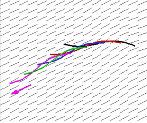
For all the stiff cases with  $\sigma _b = 0.5$, it is seen that the swimmer can simultaneously translate and rotate, seemingly subjected to a net body torque. The swimmer shape change and trajectories during the transient reorientation dynamics are shown in figures 2(a) and 2(d) for
  $\theta = {\rm \pi}/6$ (see supplementary movie 1 available at https://doi.org/10.1017/jfm.2022.621) and
  ${\rm \pi} /3$ (see supplementary movie 2), respectively. As shown in the two supplemental movies, the swimmer eventually performs steady-state undulatory swimming motions parallel to the director. We examine the time evolution of the net polymer force
  ${\bar {F}}_p(t)$ (panels b,e) and torque
  ${\bar {T}}_p(t)$ (panels c,f). To better analyse the strongly oscillating data (marked as light-colour solid lines), we calculate their means (marked as dark-colour solid lines) via the moving averaging (Hardle & Steiger Reference Hardle and Steiger1995)
 \begin{gather} \left\langle {\bar{F}}_p\right\rangle\left(t\right)=\frac{1}{T} \int_{t}^{t+T} {\bar{F}}_p \left(t'\right) {\rm d}t', \end{gather}
 \begin{gather}\left\langle{\bar{T}}_p\right\rangle\left(t\right)= \frac{1}{T} \int_{t}^{t+T} {\bar{T}}_p\left(t'\right) {\rm d}t', \end{gather}
where the sliding time window  $T=1$ is selected to be the same as the undulation period. Unlike the results of infinitely long sheets in figure 1(d), here,
  ${\bar {T}}_p$ varies asymmetrically about zero with a positive mean
  $\left \langle {\bar {T}}_p\right \rangle$ before reaching the steady states, which hence effectively drives an entire-body, counter-clockwise rotation of the swimmer. In addition, we observe the swimmer will achieve an enhanced speed at late times when swimming parallel with the director, due to a positive mean
  $\left \langle {\bar {F}}_p\right \rangle$. The reorientation dynamics of a finite-length swimmer can be also explained by examining the instantaneous polymer force distribution in the Lagrangian frame, i.e.
 \begin{equation} {\boldsymbol{F}}_p(s,t) = \int_{{\varOmega_f}} \boldsymbol{\nabla}\boldsymbol{\cdot} {{\boldsymbol{\tau}}_p}\left(\boldsymbol{x},t\right)\delta\left(\boldsymbol{X}(s) - \boldsymbol{x} \right) {\rm d}\kern0.7pt \boldsymbol{x}, \end{equation}
as shown in the insets of panels (a,d). Clearly, the Lagrangian polymer forces near the head and tail are highly aligned with the director. In the meantime, the distribution exhibits an apparent fore–aft asymmetry such that, from head to tail, not only the force magnitude increases, but also its direction completely reverses, which leads to an effective non-zero body torque.

Figure 2. Reorientation of a stiff ( ${\sigma _b} = 0.5$), finite-length (
 $L_s = 1$) swimmer in nematic LCPs (
 $\zeta = 8$,
  $\beta = 0.005$,
  $\textit {Pe} = 1$,
  $\textit {Pe}_t^{-1} = 0.02$), initially when choosing
  $\theta = {\rm \pi}/6$ (a–c) and
  ${\rm \pi} /3$ (d–f). (a,d) Sequential snapshots of swimmer shape during the transient. The background shows the typical nematic director distributions at certain time instants. The arrow denotes the swimming direction at quasi-steady states. Insets: instantaneous polymer force distributions
  $\boldsymbol {F}_p(s, t)$. The net polymer force (b,e) and torque (c,f) are plotted as functions of time, with both the instantaneous (light-colour lines) and the moving-averaged (dark-colour lines) values.
We then examine the characteristic near-body polymer force and flow field in the Eulerian frame by performing moving averages over one undulation period  $T = 1$ as
 \begin{gather} \left\langle\boldsymbol{f}_p\right\rangle\left(\boldsymbol{x},t\right)=\frac{1}{T} \int_{t}^{t+T} \boldsymbol{\nabla}\boldsymbol{\cdot} {{\boldsymbol{\tau}}_p} \left(\boldsymbol{x},t'\right) {\rm d}t', \end{gather}
 \begin{gather}\left\langle{\boldsymbol{u}}\right\rangle \left(\boldsymbol{x},t\right)=\frac{1}{T} \int_{t}^{t+T} {\boldsymbol{u}}\left(\boldsymbol{x},t'\right) {\rm d}t'. \end{gather}
For the typical case at  $\theta = {\rm \pi}/6$ shown in figure 3(a–c),
  $\left \langle \boldsymbol {f}_p\right \rangle$ reveals a strong (weak) polymer force generation near the tail (head) due to the hydrodynamic coupling between the elastic structure and the LC field. Especially, at
  $t = 0$, the resultant front-drag and rear-thrust forces are seen to be tilted with respect to the swimmer, and are consistent with the Lagrangian force distribution in figure 2. At the steady states, the near-body polymer force distribution recovers that of the parallel swimming motions along with the director by Lin et al. (Reference Lin, Chen and Gao2021). In panels (d–f), we show that the induced fluid flows remain extensile around the swimmer, with the magnitude decaying as the swimmer gradually finishes during reorientation.

Figure 3. The characteristic polymer force  $\left \langle \boldsymbol {f}_p\right \rangle$ and fluid velocity
  $\left \langle \boldsymbol {u}\right \rangle$ near the stiff (
 ${\sigma _b} = 0.5$) swimmer superimposed on their magnitudes, corresponding to the case in figure 2(a–c) when
  $\theta = {\rm \pi}/6$ initially.
Nevertheless, the dynamics of soft swimmers can be entirely different from stiff ones. As the examples shown in figure 4(a,b) where we choose  $\sigma _b$ to be two orders of magnitudes smaller than the stiff cases shown in figure 2, i.e.
  $\sigma = 0.005$, but keeping the other parameters the same, the swimmer barely moves. When tracking the body-shape change (see supplementary movies 3 and 4), it turns out that the swimmer quickly relaxes from the initially curved shape (black lines) to become approximately straight (purple lines), with small-amplitude wiggling motions. As shown in the insets, the Lagrangian force distribution
  ${\boldsymbol {F}}_p(s,t)$ along the body does not show any correlations with the nematic director field. Similar results are obtained for infinitely long soft sheets (not reported here). When performing parameter sweep, we find that non-trivial directional motions only occur when
  $\sigma _b$ goes up to
  $O(10^{-2})$. As shown in panels (c,d) for a typical case at
  $\sigma _b = 0.05$ (also see supplementary movies 5 and 6), the swimmer keeps translating and rotating but has difficultly in reaching a steady state.

Figure 4. Sequential snapshots of finite-length ( $L_s = 1$) swimmers undulating in nematic LCPs (
 $\zeta = 8$,
  $\beta = 0.005$,
  $\textit {Pe} = 1$,
  $\textit {Pe}_t^{-1} = 0.02$), when choosing the different bending stiffnesses (
 $\sigma _b = 0.005, 0.05$) and initial angles (
 $\theta = {\rm \pi}/6, {\rm \pi}/3$). The background shows the typical nematic director distributions at certain time instants. The initial shape is marked by the black colour. In panels (a,b), typical instantaneous shapes at quasi-steady states are marked by purple colour; in panels (c,d), the transient shapes are taken at
  $t = 20$ (red),
  $40$ (blue),
  $60$ (purple),
  $80$ (green), with the green arrow denoting the swimming direction at
  $t=80$. Insets in (a,b): instantaneous polymer force
  $\boldsymbol {F}_p(s, t)$ at late times.
These results suggest that performing directional motions requires a swimmer to be sufficiently stiff, which facilitates the generation of desired undulatory deformations to gain net motions (Taylor Reference Taylor1951). Once a finite-length swimmer starts moving in nematic LCPs, an asymmetric polymer force distribution automatically builds around the body with a non-zero net torque to drive the entire-body rotation. To quantitatively examine the role of  $\sigma _b$ in determining the rotational dynamics, we track the variation of the swimmer's orientation vector
  ${\boldsymbol {\hat {e}}}_U$ using a moving average with
  $T = 1$
 \begin{equation} \left\langle\phi\right\rangle(t) = \frac{1}{T} \int_{t}^{t+T} \arccos\left(|{\hat{\boldsymbol{e}}_U\left(t'\right) \boldsymbol{\cdot} \hat{\boldsymbol{e}}_x}|\right) {\rm d}t'. \end{equation}
As typical examples shown in figure 5(a,b),  $\sigma _b$ needs to go beyond
  $O(10^{-2})$ to successfully reorient when the swimmer is initially misaligned with the director. Similar reorientation dynamics has been consistently observed in the nematic regime when choosing
  $\zeta \sim O(1)$. To estimate the rotation time scale
  $\tau _R$, we fit the time-dependent curves to a saturation function of the form
  $\left \langle \phi \right \rangle (t) \sim 1 - \exp (-{t}/{\tau _R})$. As shown in panel (c) for the typical
  $\tau _R - \theta$ curves plotted at two different values of
  $\sigma _b$, we see that soft swimmers generally rotate slower than stiff ones at any given
  $\theta$. When
  $\sigma _b$ is fixed,
  $\tau _R$ monotonically increases with
  $\theta$, and the rotation time can be approximately one or two orders of magnitudes larger than the swimming period at large
  $\theta$.

Figure 5. Reorientation dynamics of the swimmer in nematic LCPs ( $\zeta = 8$) measured by the moving-averaged orientation angle
  $\left \langle \phi (t)\right \rangle$ when the initial alignment angle is chosen as
  ${\rm \pi} /6$ (a) and
  ${\rm \pi} /3$ (b) where
  $\sigma _b$ varies over three orders of magnitudes.
Note that such anisotropic swimming behaviours are similar to those of a squirmer, a coarse-grained micromechanical model of spherical active particles with specified slip velocity conditions on the surface (Blake Reference Blake1971), in nematic fluids. Several studies (Lintuvuori et al. Reference Lintuvuori, Würger and Stratford2017; Daddi-Moussa-Ider & Menzel Reference Daddi-Moussa-Ider and Menzel2018; Mandal & Mazza Reference Mandal and Mazza2021) have found that pusher-type particles with local extensile flow generation tend to align with the director while puller-type particles with contractile flows will swim perpendicular to the director. Indeed, besides the steady-state ‘parallel gait’ discussed above, Lin et al. (Reference Lin, Chen and Gao2021) reported a weak contractile flow around an undulatory swimmer that is initially aligned perpendicular to the director. However, it is unclear whether such a ‘perpendicular gait’ is stable, since slow entire-body rotation may still occur when  $\theta$ is close to
  ${\rm \pi} /2$, suggesting small disturbances could cause the rotation. Interestingly, the hydrodynamically induced reorientation dynamics for misaligned swimmers agrees with the stability condition suggested by Shi & Powers (Reference Shi and Powers2017). In their work, the imposed anchoring condition is converted to assess the exerted (local) torque per unit length as proportional to
  $\sin 2\theta$. It appears that the only stable steady-state motion (or equilibrium solution) is to swim parallel with the director, i.e.
  $\theta = 0$, such that the local torque vanishes. Nevertheless, performing quantitative analysis of the rotational stability condition for a finite-length swimmer using Doi's
  $Q$-tensor model could be laborious, and will be the subject of possible future investigations.
4. Conclusion and discussion
To summarize, we have adopted the same  $Q$-tensor model developed in our previous publication (Lin et al. Reference Lin, Chen and Gao2021) to generally study the anisotropic motions of an undulatory swimmer in nematic LCPs when the swimmer has an arbitrary alignment angle
  $\theta$ with respect to the director. For an infinite-length swimming sheet undergoing small-amplitude undulations, both the asymptotic analysis (i.e. Taylor's swimming sheet model) and IB simulations capture the similar orientation-dependent swimming speed with respect to the alignment angle, which exhibits a non-monotonic trend of enhancement and retardation. Moreover, we have demonstrated that systematically varying the bending stiffness can lead to drastic swimming behaviours when subjected to the same type of actuation. Especially, we find that the swimmer has to be sufficiently stiff to produce desired undulatory deformation to gain net motions. When initially misaligned with the nematic director, a finite-length swimmer with a minimal bending stiffness can gradually reorient before it swims steadily along with the director, when subjected to a net polymer torque arising from LCPs. Note that our
  $Q$-tensor model is essentially apolar, and strictly satisfies angular-moment conservation at the microscopic level (Feng et al. Reference Feng, Sgalari and Leal2000; Lin et al. Reference Lin, Chen and Gao2021). Hence, the net polymer torque is purely attributed to the finite-length effect that effectively breaks the fore–aft symmetry of the LCP's orientation structures surrounding the swimmer, leading to asymmetric near-body polymer force distribution. We emphasize that, besides the typical cases presented above, qualitatively similar anisotropic swimming behaviours and reorientation dynamics have been consistently observed in nematic LCPs.
Noticeably, some interesting agreements have been observed between the Doi- and EL-type models that incorporate different mechanisms for resolving the reciprocal coupling between the suspended polymers, moving structures and fluid flows. For example, we have shown that the asymptotic solution of the mean swimming speed of Taylor's swimming sheet in (3.4) has the same  $\theta$-dependency as that derived from an EL model by Shi & Powers (Reference Shi and Powers2017) in the transversely isotropic limit. Also, the reorientation of a misaligned finite-length swimmer captured in this study confirms the stability condition derived by the same authors in terms of the exerted local torque by LCPs arising from the anchoring conditions. However, we emphasize that Doi's
  $Q$-tensor model does not require enforcement of the rods’ orientation directions along the swimmer body via any anchoring conditions. Instead, the variations of orientational structures are simultaneously determined by the induced near-body fluid flows and the LCP's intrinsic nematic elasticity, which is mainly characterized by the MS potential and the rotational diffusion. Without specifying an explicit structure–orientation coupling at the solid boundary, the produced extra stresses effectively drive the fluid motions in a mean-field fashion, and couple with the undulatory swimming motions hydrodynamically via the no-slip conditions.
To seek further connections between the two different LC models, one may consider adding the contributions of distortion elasticity to the MS potential (Greco & Marrucci Reference Greco and Marrucci1992) in Doi's model, leading to equations that can mathematically recover the director formulation of the EL model in the limit of weak flow and mild spatial distortion (Feng et al. Reference Feng, Sgalari and Leal2000). Also, the high-order orientational derivatives in the distortion elastic terms require imposition of additional boundary conditions for the orientation field, equivalent to applying anchoring conditions. Then it is straightforward to examine how swimming dynamics will change in response to the additional structure–orientation coupling. Moreover, it will be intriguing to study undulatory swimming motions in three dimensions where the nematic field may exhibit far more complex topological structures to impact the resultant FSIs and associated gait stability.

Figure 6. Rotation time  $\tau _R$ as a function of the initial alignment angle
  $\theta$ for
  $\sigma _b = 0.2, 0.5$.
Supplementary movies
Supplementary movies are available at https://doi.org/10.1017/jfm.2022.621.
Funding
Z.L. acknowledges the National Natural Science Foundations of China grant No. 12172327 and No. 12132015. T.G. acknowledges the National Science Foundation grant No. 1943759 which partially supports this work.
Declaration of interests
The authors report no conflict of interest.
Appendix A. Numerical method validation
We use the same spectral IB method developed by Lin et al. (Reference Lin, Chen and Gao2021). Here, we show two benchmark studies for an infinite swimming sheet in both isotropic and anisotropic fluids. As shown in figure 7, we first study the undulatory swimming motions of infinite flexible sheet in an Oldroyd-B (OB) fluid where the dimensionless Deborah ( ${De}$) number, playing a similar role as
  $\textit {Pe}$ in the LC cases, is defined as the wave frequency by the OB fluid relaxation time. We measured the mean centre-of-mass swimming speed
  $U_{OB}$ of the swimmer, and compared the speed ratio with the numerical data by Salazar, Roma & Ceniceros (Reference Salazar, Roma and Ceniceros2016) and the asymptotic results for Taylor's swimming sheet by Lauga (Reference Lauga2007)
 \begin{equation} \frac{{U}_{OB}}{{U}_{N}}=\frac{1+\left(\dfrac{\eta_{s}}{\eta_{s}+\eta_{p}}\right) {De}^{2}}{1+{De}^{2}}, \end{equation}
where  $\eta _s$ and
  $\eta _p$ respectively represent the solvent and polymer contributions to the viscosity. The Newtonian speed
  $U_N$ can be derived as
 \begin{equation} {U}_{N}=\frac{1}{2}\left(\frac{\omega}{k}\right)(A k)^{2}+{O}\left(A k\right)^{4}. \end{equation}
Next, we performed the convergence tests for an infinite stiff swimming sheet swimming in LCPs as shown in figure 8, where we examine the time-dependent velocity components by varying the grid width, time step, domain size and stiffness separately.

Figure 7. Time-averaged centre-of-mass speed  $U_{OB}$ for undulatory swimming motion in an OB fluid when choosing
  ${De} = 1$.

Figure 8. Convergence tests with the time-dependent centre-of-mass velocity  $u_x$ and
  $u_y$ when changing (a) the Eulerian grid width, (b) the domain size and (c) the bending stiffness
  $\sigma _b$. These parameters are fixed:
  $\sigma _s = 500$,
  ${\sigma _b} = 0.5$,
  $A= 0.01$,
  $\textit {Pe} = 1$,
  $\textit {Er} = 1$,
  $\zeta = 8$,
  ${\textit {Pe}_t}^{-1} = 0.02$,
  $\beta = 0.0005$ and
  $\theta = {\rm \pi}/6$.
Appendix B. Asymptotic analysis
In the moving frame of the swimmer, we consider the vertical displacement of an infinitely long wavy sheet with the described travelling-wave motion as  $y(x, t)= A \sin (k x - \omega t)$. We then rescale it as
 \begin{equation} y(x, t) = \varepsilon \sin (x - t), \end{equation}
by choosing  $1/k$ the length scale,
  $1/\omega$ the time scale and
  $\omega /k$ the velocity scale. To model Taylor's swimming sheet, we assume a small amplitude
  $\varepsilon = Ak \ll 1$. Following the classical work by Lauga (Reference Lauga2007), we adopt a streamfunction
  $\varphi (x, y, t)$ to describe the two-dimensional incompressible flow as
 \begin{equation} {\boldsymbol{u}} = \boldsymbol{\nabla} \times \left( {\varphi {{\hat{\boldsymbol{e}}}_z}} \right). \end{equation}
Hence, the velocity components can be computed as  $u_{x} = \partial \varphi / \partial y$,
  $u_{y} = -\partial \varphi / \partial x$. The boundary conditions for
  $\varphi (x, y, t)$ arise from conditions at infinity and on the undulatory sheet with a steady speed
  $-U_{LC} {\hat {\boldsymbol {e}}}_{x}$. Then the far-field condition at
  $y=\infty$ becomes
 \begin{equation} \left.\boldsymbol{\nabla} \varphi\right|_{(x, \infty)}=U_{LC} {\hat{\boldsymbol{e}}}_{y}. \end{equation}
On the swimming sheet, the no-slip velocity condition is imposed as
 \begin{equation} \left.\boldsymbol{\nabla} \varphi\right|_{(x, \varepsilon \sin (x-t))}=\varepsilon \cos (x-t) {\hat{\boldsymbol{e}}}_{x}. \end{equation}
Recalling the forced Stokes equation
 \begin{equation} \boldsymbol{\nabla} p=\Delta \boldsymbol{u}+\textit{Er} \,\boldsymbol{\nabla}\boldsymbol{\cdot}\boldsymbol{\tau}_{p}, \end{equation}
where polymer stress, when ignoring  $\beta$, is given as
 \begin{equation} \boldsymbol{\tau}_{p}=\left(\boldsymbol{D}-\frac{\boldsymbol{\mathsf{I}}}{2}\right)-\zeta\left(\boldsymbol{D} \boldsymbol{\cdot} \boldsymbol{D}-\boldsymbol{D}: \boldsymbol{S}\right). \end{equation}
We focus on the effects of alignment angle  $\theta$ on swimming speed in the nematic regime, and adopt a classical quadratic closure to approximate the fourth moment
  $\boldsymbol {S}$ (Doi & Edwards Reference Doi and Edwards1988) as
 \begin{equation} \boldsymbol{S}=\boldsymbol{DD}, \end{equation}
which facilitates analytical manipulation in the following. Note that this closure becomes more and more accurate in deep nematic when  $\zeta \gg \zeta _c$. Now the evolution equation of
  $\boldsymbol {D}$ reads
 \begin{equation} \mathop{\boldsymbol{D}}\limits^{\boldsymbol{\nabla}}+2 \boldsymbol{E}: \boldsymbol{S}={-}\frac{1}{\textit{Pe}}\left(\boldsymbol{D}-\frac{\boldsymbol{\mathsf{I}}}{2}\right)+ \frac{\zeta}{\textit{Pe}}(\boldsymbol{D} \boldsymbol{\cdot} \boldsymbol{D}-\boldsymbol{D}: \boldsymbol{S}), \end{equation}
with  $\mathop {\boldsymbol {D}}\limits ^{\boldsymbol {\nabla }}$ an upper-convected time derivative. When applying the curl on both sides of (B5), we have
 \begin{equation} \boldsymbol{\nabla} \times (\boldsymbol{\nabla}\boldsymbol{\cdot} \boldsymbol{\tau}_{p})= \frac{1}{\textit{Er}} \nabla^{4} \varphi {{\hat{\boldsymbol{e}}}_z}. \end{equation}
 Next, we expand all the variables with  $\varepsilon$ to the second order and
  $\delta = {\zeta ^{-1}}$(
 $\zeta \gg 1$) to the first order, i.e.
 \begin{gather} \varphi=\varepsilon (\varphi^{(10)}+\delta \varphi^{(11)})+\varepsilon^{2} (\varphi^{(20)}+\delta \varphi^{(21)})+O\left(\varepsilon^{3}, \delta^2\right), \end{gather}
 \begin{gather}{\boldsymbol{\tau}} = ({{\boldsymbol{\tau}}^{(00)}}+\delta {{\boldsymbol{\tau}}^{(01)}}) + \varepsilon ({{\boldsymbol{\tau}}^{(10)}}+\delta{{\boldsymbol{\tau}}^{(11)}}) + {\varepsilon ^2}({{\boldsymbol{\tau}}^{(20)}}+\delta{{\boldsymbol{\tau}}^{(21)}})+ O({\varepsilon ^3}, \delta^2), \end{gather}
 \begin{gather}{\boldsymbol{D}} = ({\boldsymbol{\mathsf{D}}^{(00)}}+\delta {\boldsymbol{\mathsf{D}}^{(01)}}) + \varepsilon ({\boldsymbol{\mathsf{D}}^{(10)}}+\delta {\boldsymbol{\mathsf{D}}^{(11)}}) + {\varepsilon ^2}({\boldsymbol{\mathsf{D}}^{(20)}}+\delta {\boldsymbol{\mathsf{D}}^{(21)}}) + O({\varepsilon ^3}, \delta^2), \end{gather}
 \begin{gather}U_{LC}=\varepsilon (U_{LC}^{(10)}+\delta U_{LC}^{(11)})+\varepsilon^{2} (U_{LC}^{(20)}+\delta U_{LC}^{(21)})+O\left(\varepsilon^{3}, \delta^2\right). \end{gather}
After some manipulations, we can derive the following governing equations at different orders:
 $O(\varepsilon ^{0}, \delta ^{-1})$ order
 \begin{equation} \sum_{k+l=0} \left(\boldsymbol{\mathsf{D}}^{(k0)} \boldsymbol{\cdot} \boldsymbol{\mathsf{D}}^{(l0)} - \boldsymbol{\mathsf{D}}^{(k0)} : \boldsymbol{S}^{(l0)}\right) = \boldsymbol{0}. \end{equation}
  $O(\varepsilon ^{0}, \delta ^{0})$ order
 \begin{equation} \boldsymbol{\tau}_{p}^{(00)}=\left(\boldsymbol{\mathsf{D}}^{(00)}-\frac{\boldsymbol{\mathsf{I}}}{2}\right) - \sum_{k+l=0} \sum_{i+j=1} \left(\boldsymbol{\mathsf{D}}^{(k i)} \cdot \boldsymbol{\mathsf{D}}^{(l j)} - \boldsymbol{\mathsf{D}}^{(k i)} : \boldsymbol{S}^{(l j)}\right), \end{equation}
 \begin{align} &\frac{\partial \boldsymbol{\mathsf{D}}^{(00)}}{\partial t}+ \sum_{k+l=0} \sum_{i+j=0}\left[\boldsymbol{u}^{(k i)} \boldsymbol{\cdot}\boldsymbol{\nabla} \boldsymbol{\mathsf{D}}^{(l j)}-\left(\boldsymbol{\mathsf{D}}^{(k i)} \boldsymbol{\cdot}\boldsymbol{\nabla} \boldsymbol{u}^{(l j)}+\boldsymbol{\nabla} {\boldsymbol{u}^{(l j)}}^{{{\rm T}}} \boldsymbol{\cdot} \boldsymbol{\mathsf{D}}^{(k i)}\right)+2 \boldsymbol{E}^{(k i)}: \boldsymbol{S}^{(l j)}\right]\nonumber\\ &\quad ={-}\frac{1}{\textit{Pe}}\left(\boldsymbol{\mathsf{D}}^{(00)}-\frac{\boldsymbol{\mathsf{I}}}{2}\right)+\frac{1}{\textit{Pe}} \sum_{k+l=0} \sum_{i+j=1}\left(\boldsymbol{\mathsf{D}}^{(k i)} \boldsymbol{\cdot} \boldsymbol{\mathsf{D}}^{(l j)}-\boldsymbol{\mathsf{D}}^{(k i)}: \boldsymbol{S}^{(l j)}\right). \end{align}
  $O(\varepsilon ^{0}, \delta ^{1})$ order
 \begin{equation} \boldsymbol{\tau}_{p}^{(01)}=\boldsymbol{\mathsf{D}}^{(01)} - \sum_{k+l=0} \sum_{i+j=2} \left(\boldsymbol{\mathsf{D}}^{(k i)} \boldsymbol{\cdot} \boldsymbol{\mathsf{D}}^{(l j)} - \boldsymbol{\mathsf{D}}^{(k i)} : \boldsymbol{S}^{(l j)}\right), \end{equation}
 \begin{align} &\frac{\partial \boldsymbol{\mathsf{D}}^{(01)}}{\partial t}+\sum_{k+l=0}\sum_{i+j=1}\left[\boldsymbol{u}^{(k i)} \boldsymbol{\cdot}\boldsymbol{\nabla} \boldsymbol{\mathsf{D}}^{(l j)}-\left(\boldsymbol{\mathsf{D}}^{(k i)} \boldsymbol{\cdot}\boldsymbol{\nabla} \boldsymbol{u}^{(l j)}+\boldsymbol{\nabla} {\boldsymbol{u}^{(l j)}}^{{{\rm T}}} \boldsymbol{\cdot} \boldsymbol{\mathsf{D}}^{(k i)}\right)+2 \boldsymbol{E}^{(k i)}: \boldsymbol{S}^{(l j)}\right]\nonumber\\ &\quad={-}\frac{1}{\textit{Pe}}\boldsymbol{\mathsf{D}}^{(01)}+\frac{1}{\textit{Pe}} \sum_{k+l=0} \sum_{i+j=2}\left(\boldsymbol{\mathsf{D}}^{(k i)} \boldsymbol{\cdot} \boldsymbol{\mathsf{D}}^{(l j)}-\boldsymbol{\mathsf{D}}^{(k i)}: \boldsymbol{S}^{(l j)}\right). \end{align}
  $O(\varepsilon ^{1}, \delta ^{-1})$ order
 \begin{equation} \sum_{k+l=1} \left(\boldsymbol{\mathsf{D}}^{(k0)} \boldsymbol{\cdot} \boldsymbol{\mathsf{D}}^{(l0)} - \boldsymbol{\mathsf{D}}^{(k0)} : \boldsymbol{S}^{(l0)}\right) = \boldsymbol{0}. \end{equation}
  $O(\varepsilon ^{1}, \delta ^{0})$ order
 \begin{equation} \boldsymbol{\tau}_{p}^{(10)}=\boldsymbol{\mathsf{D}}^{(10)} - \sum_{k+l=1} \sum_{i+j=1} \left(\boldsymbol{\mathsf{D}}^{(k i)} \boldsymbol{\cdot} \boldsymbol{\mathsf{D}}^{(l j)} - \boldsymbol{\mathsf{D}}^{(k i)} : \boldsymbol{S}^{(l j)}\right), \end{equation}
 \begin{align} &\frac{\partial \boldsymbol{\mathsf{D}}^{(10)}}{\partial t}+\sum_{k+l=1}\sum_{i+j=0}\left[\boldsymbol{u}^{(k i)} \boldsymbol{\cdot}\boldsymbol{\nabla} \boldsymbol{\mathsf{D}}^{(l j)}-\left(\boldsymbol{\mathsf{D}}^{(k i)} \boldsymbol{\cdot}\boldsymbol{\nabla} \boldsymbol{u}^{(l j)}+\boldsymbol{\nabla} {\boldsymbol{u}^{(l j)}}^{{{\rm T}}} \boldsymbol{\cdot} \boldsymbol{\mathsf{D}}^{(k i)}\right)+2 \boldsymbol{E}^{(k i)}: \boldsymbol{S}^{(l j)}\right]\nonumber\\ &\quad ={-}\frac{1}{\textit{Pe}}\boldsymbol{\mathsf{D}}^{(10)}+\frac{1}{\textit{Pe}} \sum_{k+l=1} \sum_{i+j=1}\left(\boldsymbol{\mathsf{D}}^{(k i)} \boldsymbol{\cdot} \boldsymbol{\mathsf{D}}^{(l j)}-\boldsymbol{\mathsf{D}}^{(k i)}: \boldsymbol{S}^{(l j)}\right). \end{align}
  $O(\varepsilon ^{1}, \delta ^{1})$ order
 \begin{equation} \boldsymbol{\tau}_{p}^{(11)}=\boldsymbol{\mathsf{D}}^{(11)} - \sum_{k+l=1} \sum_{i+j=2} \left(\boldsymbol{\mathsf{D}}^{(k i)} \boldsymbol{\cdot} \boldsymbol{\mathsf{D}}^{(l j)} - \boldsymbol{\mathsf{D}}^{(k i)} : \boldsymbol{S}^{(l j)}\right), \end{equation}
 \begin{align} &\frac{\partial \boldsymbol{\mathsf{D}}^{(11)}}{\partial t}+\sum_{k+l=1}\sum_{i+j=1}\left[\boldsymbol{u}^{(k i)} \boldsymbol{\cdot}\boldsymbol{\nabla} \boldsymbol{\mathsf{D}}^{(l j)}-\left(\boldsymbol{\mathsf{D}}^{(k i)} \boldsymbol{\cdot}\boldsymbol{\nabla} \boldsymbol{u}^{(l j)}+\boldsymbol{\nabla} {\boldsymbol{u}^{(l j)}}^{{{\rm T}}} \boldsymbol{\cdot} \boldsymbol{\mathsf{D}}^{(k i)}\right)+2 \boldsymbol{E}^{(k i)}: \boldsymbol{S}^{(l j)}\right]\nonumber\\ &\quad ={-}\frac{1}{\textit{Pe}}\boldsymbol{\mathsf{D}}^{(11)}+\frac{1}{\textit{Pe}} \sum_{k+l=1} \sum_{i+j=2}\left(\boldsymbol{\mathsf{D}}^{(k i)} \boldsymbol{\cdot} \boldsymbol{\mathsf{D}}^{(l j)}-\boldsymbol{\mathsf{D}}^{(k i)}: \boldsymbol{S}^{(l j)}\right). \end{align}
  $O(\varepsilon ^{2}, \delta ^{-1})$ order
 \begin{equation} \sum_{k+l=2} \left(\boldsymbol{\mathsf{D}}^{(k0)} \boldsymbol{\cdot} \boldsymbol{\mathsf{D}}^{(l0)} - \boldsymbol{\mathsf{D}}^{(k0)} : \boldsymbol{S}^{(l0)}\right) = \boldsymbol{0}. \end{equation}
  $O(\varepsilon ^{2}, \delta ^{0})$ order
 \begin{equation} \boldsymbol{\tau}_{p}^{(20)}=\boldsymbol{\mathsf{D}}^{(20)} - \sum_{k+l=2} \sum_{i+j=1} \left(\boldsymbol{\mathsf{D}}^{(k i)} \boldsymbol{\cdot} \boldsymbol{\mathsf{D}}^{(l j)} - \boldsymbol{\mathsf{D}}^{(k i)} : \boldsymbol{S}^{(l j)}\right), \end{equation}
 \begin{align} &\frac{\partial \boldsymbol{\mathsf{D}}^{(20)}}{\partial t}+\sum_{k+l=2}\sum_{i+j=0}\left[\boldsymbol{u}^{(k i)} \boldsymbol{\cdot}\boldsymbol{\nabla} \boldsymbol{\mathsf{D}}^{(l j)}-\left(\boldsymbol{\mathsf{D}}^{(k i)} \boldsymbol{\cdot}\boldsymbol{\nabla} \boldsymbol{u}^{(l j)}+\boldsymbol{\nabla} {\boldsymbol{u}^{(l j)}}^{{{\rm T}}} \boldsymbol{\cdot} \boldsymbol{\mathsf{D}}^{(k i)}\right)+2 \boldsymbol{E}^{(k i)}: \boldsymbol{S}^{(l j)}\right]\nonumber\\ &\quad ={-}\frac{1}{\textit{Pe}}\boldsymbol{\mathsf{D}}^{(20)}+\frac{1}{\textit{Pe}} \sum_{k+l=2} \sum_{i+j=1}\left(\boldsymbol{\mathsf{D}}^{(k i)} \boldsymbol{\cdot} \boldsymbol{\mathsf{D}}^{(l j)}-\boldsymbol{\mathsf{D}}^{(k i)}: \boldsymbol{S}^{(l j)}\right). \end{align}
  $O(\varepsilon ^{2}, \delta ^{1})$ order
 \begin{equation} \boldsymbol{\tau}_{p}^{(21)}=\boldsymbol{\mathsf{D}}^{(21)} - \sum_{k+l=2} \sum_{i+j=2} \left(\boldsymbol{\mathsf{D}}^{(k i)} \boldsymbol{\cdot} \boldsymbol{\mathsf{D}}^{(l j)} - \boldsymbol{\mathsf{D}}^{(k i)} : \boldsymbol{S}^{(l j)}\right), \end{equation}
 \begin{align} &\frac{\partial \boldsymbol{\mathsf{D}}^{(21)}}{\partial t}+\sum_{k+l=2}\sum_{i+j=1}\left[\boldsymbol{u}^{(k i)} \boldsymbol{\cdot}\boldsymbol{\nabla} \boldsymbol{\mathsf{D}}^{(l j)}-\left(\boldsymbol{\mathsf{D}}^{(k i)} \boldsymbol{\cdot}\boldsymbol{\nabla} \boldsymbol{u}^{(l j)}+\boldsymbol{\nabla} {\boldsymbol{u}^{(l j)}}^{{{\rm T}}} \boldsymbol{\cdot} \boldsymbol{\mathsf{D}}^{(k i)}\right)+2 \boldsymbol{E}^{(k i)}: \boldsymbol{S}^{(l j)}\right]\nonumber\\ &\quad ={-}\frac{1}{\textit{Pe}}\boldsymbol{\mathsf{D}}^{(21)}+\frac{1}{\textit{Pe}} \sum_{k+l=2} \sum_{i+j=2}\left(\boldsymbol{\mathsf{D}}^{(k i)} \boldsymbol{\cdot} \boldsymbol{\mathsf{D}}^{(l j)}-\boldsymbol{\mathsf{D}}^{(k i)}: \boldsymbol{S}^{(l j)}\right). \end{align}
At  $O(\varepsilon ^{0})$, we can solve for homogeneous solutions. Now the boundary conditions at
  $O(\varepsilon ^{1})$ become
 $O(\varepsilon ^{1}, \delta ^{0})$ order
 \begin{gather} \left.\boldsymbol{\nabla} \varphi^{(10)}\right|_{(x, \infty)}=U_{LC}^{(10)} {\hat{\boldsymbol{e}}}_{y}, \end{gather}
 \begin{gather}\left.\boldsymbol{\nabla}\varphi^{(10)}\right|_{(x, 0)}=\cos (x-t) {\hat{\boldsymbol{e}}}_{x}. \end{gather}
  $O(\varepsilon ^{1}, \delta ^{1})$ order
 \begin{gather} \left.\boldsymbol{\nabla} \varphi^{(11)}\right|_{(x, \infty)}=U_{LC}^{(11)} {\hat{\boldsymbol{e}}}_{y}, \end{gather}
 \begin{gather}\left.\boldsymbol{\nabla} \varphi^{(11)}\right|_{(x, 0)}=\boldsymbol{0}. \end{gather}
Note that, in the above, instead of being satisfied exactly along the wavy body, the no-slip boundary condition is projected onto the  $x$-axis, i.e. at
  $y=0$. And at
  $O(\varepsilon ^{2})$, they take the form
 $O(\varepsilon ^{2}, \delta ^{0})$ order
 \begin{gather} \left.\boldsymbol{\nabla} \varphi^{(20)}\right|_{(x, \infty)}=U_{LC}^{(20)} {\hat{\boldsymbol{e}}}_{y}, \end{gather}
 \begin{gather}\left.\boldsymbol{\nabla} \varphi^{(20)}\right|_{(x, 0)}={-}\sin (x-t) \boldsymbol{\nabla} \left(\frac{\partial \varphi^{(10)}}{\partial y}\right)|_{(x, 0)}. \end{gather}
  $O(\varepsilon ^{2}, \delta ^{1})$ order
 \begin{gather} \left.\boldsymbol{\nabla} \varphi^{(21)}\right|_{(x, \infty)}=U_{LC}^{(21)} {\hat{\boldsymbol{e}}}_{y}, \end{gather}
 \begin{gather}\left.\boldsymbol{\nabla} \varphi^{(21)}\right|_{(x, 0)}={-}\sin (x-t) \boldsymbol{\nabla} \left.\left(\frac{\partial \varphi^{(11)}}{\partial y}\right)\right|_{(x, 0)}. \end{gather}
To proceed, we choose to decompose the steady-state configuration tensor as
 \begin{equation} \boldsymbol{\mathsf{D}}^{(00)} = \boldsymbol{\mathsf{M}}(\theta)\overline{\boldsymbol{\mathsf{D}}^{(00)}}\boldsymbol{\mathsf{M}}^{{-}1}(\theta) \end{equation}
where  $\overline {\boldsymbol{\mathsf{D}}^{(00)}}={\rm diag}(\overline {{{{\mathsf{D}}_{11}^{(00)}}}}, 1-\overline {{{{\mathsf{D}}_{11}^{(00)}}}})$,
  $\overline {{{{\mathsf{D}}_{11}^{(00)}}}}>1/2$ and the rotation matrix
  $\boldsymbol{\mathsf{M}}(\theta ) = \left (\begin {smallmatrix} {\cos \theta } & {-\sin \theta } \\ {\sin \theta } & {\cos \theta } \end {smallmatrix}\right )$. Then we solve
  $\overline {\boldsymbol{\mathsf{D}}^{(00)}}$ via (B14) to obtain
 \begin{align} \boldsymbol{0}&=\boldsymbol{\mathsf{M}}^{{-}1}(\theta)\sum_{k+l=0} \left(\boldsymbol{\mathsf{D}}^{(k0)} \boldsymbol{\cdot} \boldsymbol{\mathsf{D}}^{(l0)} - \boldsymbol{\mathsf{D}}^{(k0)} : \boldsymbol{S}^{(l0)}\right) \boldsymbol{\mathsf{M}}(\theta) \nonumber\\ &=\sum_{k+l=0} \left(\overline{\boldsymbol{\mathsf{D}}^{(k0)}} \boldsymbol{\cdot} \overline{\boldsymbol{\mathsf{D}}^{(l0)}}-\sum_{l_1+l_2=0}\left(\overline{\boldsymbol{\mathsf{D}}^{(k0)}} : \overline{\boldsymbol{\mathsf{D}}^{(l_1 0)}}\right) \overline{\boldsymbol{\mathsf{D}}^{(l_2 0)}}\right), \end{align}
which yields the equilibrium solutions
 \begin{equation} \overline{\boldsymbol{\mathsf{D}}^{(00)}} = \begin{pmatrix}{1} & {0} \\ {0} & {0}\end{pmatrix}, \quad \overline{\boldsymbol{\mathsf{D}}^{(01)}} = \begin{pmatrix}{-\frac{1}{2}} & {0} \\ {0} & {\frac{1}{2}}\end{pmatrix}, \quad \overline{\boldsymbol{\mathsf{D}}^{(02)}} = \begin{pmatrix}{-\frac{1}{4}} & {0} \\ {0} & {\frac{1}{4}}\end{pmatrix}. \end{equation}
We denote
 \begin{equation} {\boldsymbol{F}} = \boldsymbol{\nabla}\boldsymbol{u} = \begin{pmatrix} {F_{11}} & {F_{12}} \\ {F_{21}} & {-F_{11}} \end{pmatrix}. \end{equation}
At  $O(\varepsilon ^{1}, \delta ^{0})$, we solve configuration tensor
  $\overline {\boldsymbol{\mathsf{D}}^{(10)}}$ as
 \begin{equation} \overline{\boldsymbol{\mathsf{D}}^{(10)}} = \overline{{\mathsf{D}}^{(10)}_{12}}\begin{pmatrix}{0} & {1} \\ {1} & {0}\end{pmatrix}, \end{equation}
which leads to  $\overline {\boldsymbol {\tau }_{p}^{(10)}}=\boldsymbol {0}$ and
  $\overline {{\mathsf{D}}^{(11)}_{11}}=0$. We can further derive
 \begin{equation} \nabla^{4} \varphi^{(10)} = 0. \end{equation}
Given the boundary conditions, we obtain the solution
 \begin{gather} \varphi^{(10)}(x,y,t) = (1+y){\rm e}^{{-}y}\sin (x-t), \end{gather}
 \begin{gather}U_{LC}^{(10)} = 0, \end{gather}
leading to the solution
 \begin{equation} \overline{{\mathsf{D}}_{12}^{(10)}} = y{\rm e}^{{-}y}\cos (x-t+2\theta)+{\rm e}^{{-}y}\cos (x-t). \end{equation}
At  $O(\varepsilon ^{1}, \delta ^{1})$ order, using (B22), we can derive
 \begin{equation} \overline{\boldsymbol{\tau}_{p}^{(11)}}= \overline{{\mathsf{D}}^{(12)}_{11}}\begin{pmatrix}{1} & {0} \\ {0} & {-1}\end{pmatrix}. \end{equation}
Using (B23), we obtain the equations
 \begin{gather} \frac{1}{P e}\overline{\tau_{p,11}^{(11)}}-2\overline{F_{11}^{(10)}}=0, \end{gather}
 \begin{gather}\frac{\partial \overline{{\mathsf{D}}_{12}^{(11)}}}{\partial t}- \overline{F_{12}^{(11)}}+\frac{1}{2}\left(\overline{F_{12}^{(10)}}-\overline{F_{21}^{(10)}}\right)=0. \end{gather}
Then we can obtain the solutions
 \begin{equation} \overline{\tau_{p,11}^{(11)}}=\overline{{\mathsf{D}}^{(12)}_{11}}={-}2y{\rm e}^{{-}y}\cos (x-t+2\theta){\textit{Pe}}, \end{equation}
which leads to
 \begin{equation} \nabla^{4} \varphi^{(11)} = 4(y-1){\rm e}^{{-}y}\sin (x-t+4\theta){\textit{Er}}\,{\textit{Pe}}. \end{equation}
Given the boundary conditions in (B31)–(B32), we obtain the solution
 \begin{gather} \varphi^{(11)}(x,y,t) = \tfrac{1}{6}y^{3}{\rm e}^{{-}y}\sin (x-t+4\theta){\textit{Er}}\,{\textit{Pe}}, \end{gather}
 \begin{gather}U_{LC}^{(11)} = 0. \end{gather}
Substituting (B51) into (B47), we can derive the solution
 \begin{align} \overline{{\mathsf{D}}_{12}^{(11)}} &= \tfrac{1}{6}{\textit{Er}}\,{\textit{Pe}} \left[\left(y^{3}-3y^{2}+ \tfrac{3}{2}y\right){\rm e}^{{-}y}\cos (x-t+6\theta) \right.\nonumber\\ &\left.\quad +(3y^{2}-3y){\rm e}^{{-}y}\cos (x-t+4\theta)+\tfrac{3}{2}y{\rm e}^{{-}y}\cos (x-t+2\theta)\right]-{\rm e}^{{-}y}\cos (x-t). \end{align}
 At  $O(\varepsilon ^{2}, \delta ^{0})$, we solve configuration tensor
  $\overline {\boldsymbol{\mathsf{D}}^{(20)}}$ via (B24) and get the form
 \begin{equation} \overline{{\mathsf{D}}_{11}^{(20)}} ={-}\overline{{\mathsf{D}}^{(10)}_{12}}^{2}. \end{equation}
Using (B25), we have
 \begin{equation} \overline{\boldsymbol{\tau}_{p}^{(20)}}=\left(\overline{{\mathsf{D}}^{(21)}_{11}}-2 \overline{{\mathsf{D}}^{(20)}_{11}}+2 \overline{{\mathsf{D}}^{(10)}_{12}} \overline{{\mathsf{D}}^{(11)}_{12}}-\overline{{\mathsf{D}}^{(10)}_{12}}^{2}\right)\begin{pmatrix}{1} & {0} \\ {0} & {-1}\end{pmatrix}. \end{equation}
Using (B26), we can derive the equations
 \begin{gather} \frac{\partial \overline{{\mathsf{D}}_{11}^{(20)}}}{\partial t}+2\overline{F_{12}^{(10)}}\overline{{\mathsf{D}}_{12}^{(10)}}+\frac{1}{P e}\overline{\tau_{p,11}^{(20)}}=0, \end{gather}
 \begin{gather}\frac{\partial \overline{{\mathsf{D}}_{12}^{(20)}}}{\partial t}+\left(\boldsymbol{u}^{(10)} \boldsymbol{\cdot} \boldsymbol{\nabla}\right)\overline{{\mathsf{D}}_{12}^{(10)}}-\overline{F_{12}^{(20)}}+2 \overline{E_{11}^{(10)}}\overline{{\mathsf{D}}_{12}^{(10)}}=0. \end{gather}
Then we can obtain
 \begin{equation} \overline{\tau_{p,11}^{(20)}}={-}{\textit{Pe}}\left(\frac{\partial \overline{{\mathsf{D}}_{11}^{(20)}}}{\partial t}+2\overline{F_{12}^{(10)}}\overline{{\mathsf{D}}_{12}^{(10)}}\right)=0, \end{equation}
leading to
 \begin{equation} \nabla^{4} \varphi^{(20)} = 0. \end{equation}
Applying the boundary conditions (B33)–(B34), we obtain
 \begin{gather} \varphi^{(20)}(x,y,t)={-}\tfrac{1}{2}y{\rm e}^{{-}2y}\cos (2x-2t)+\tfrac{1}{2}y, \end{gather}
 \begin{gather}U_{LC}^{(20)} = \tfrac{1}{2}. \end{gather}
 At  $O(\varepsilon ^{2}, \delta ^{1})$, using (B27), we first derive the equations
 \begin{align} \left.\begin{aligned}
&\overline{\tau_{p,11}^{(21)}}=\overline{{\mathsf{D}}_{11}^{(22)}}-2\overline{{\mathsf{D}}_{11}^{(21)}}-2\overline{{\mathsf{D}}_{12}^{(10)}}\overline{{\mathsf{D}}_{12}^{(11)}}+2\overline{{\mathsf{D}}_{12}^{(10)}}\overline{{\mathsf{D}}_{12}^{(12)}}+{\overline{{\mathsf{D}}_{12}^{(11)}}}^2-\frac{1}{2}{\overline{{\mathsf{D}}_{12}^{(10)}}}^2,
\\
&\overline{\tau_{p,12}^{(21)}}=2\overline{{\mathsf{D}}_{12}^{(10)}}\overline{{\mathsf{D}}_{11}^{(12)}},
\\
&\overline{\tau_{p,22}^{(21)}}={-}\overline{\tau_{p,11}^{(21)}}.
\end{aligned} \right\} \end{align}
\begin{align} \left.\begin{aligned}
&\overline{\tau_{p,11}^{(21)}}=\overline{{\mathsf{D}}_{11}^{(22)}}-2\overline{{\mathsf{D}}_{11}^{(21)}}-2\overline{{\mathsf{D}}_{12}^{(10)}}\overline{{\mathsf{D}}_{12}^{(11)}}+2\overline{{\mathsf{D}}_{12}^{(10)}}\overline{{\mathsf{D}}_{12}^{(12)}}+{\overline{{\mathsf{D}}_{12}^{(11)}}}^2-\frac{1}{2}{\overline{{\mathsf{D}}_{12}^{(10)}}}^2,
\\
&\overline{\tau_{p,12}^{(21)}}=2\overline{{\mathsf{D}}_{12}^{(10)}}\overline{{\mathsf{D}}_{11}^{(12)}},
\\
&\overline{\tau_{p,22}^{(21)}}={-}\overline{\tau_{p,11}^{(21)}}.
\end{aligned} \right\} \end{align}
Using (B28), we can further derive
 \begin{align} \left.\begin{aligned}
&\displaystyle\frac{\partial
\overline{{\mathsf{D}}_{11}^{(21)}}}{\partial
t}-2\overline{E_{11}^{(20)}}+2\overline{F_{12}^{(11)}}\overline{{\mathsf{D}}_{12}^{(10)}}+2\overline{F_{12}^{(10)}}\overline{{\mathsf{D}}_{12}^{(11)}}-2\overline{E_{12}^{(10)}}\overline{{\mathsf{D}}_{12}^{(10)}}+\frac{1}{P
e}\overline{\tau_{p,11}^{(21)}}=0, \\
&\displaystyle\frac{\partial
\overline{{\mathsf{D}}_{12}^{(21)}}}{\partial
t}+\left(\boldsymbol{u}^{(10)}
\boldsymbol{\cdot}\boldsymbol{\nabla}\right)\overline{{\mathsf{D}}_{12}^{(11)}}+\left(\boldsymbol{u}^{(11)}
\boldsymbol{\cdot}\boldsymbol{\nabla}\right)\overline{{\mathsf{D}}_{12}^{(10)}}-\overline{F_{12}^{(21)}}-\frac{1}{2}\left(\overline{F_{21}^{(20)}}-\overline{F_{12}^{(20)}}\right)
\\ \displaystyle&\quad
+2\overline{{\mathsf{D}}_{12}^{(10)}}\left(\overline{E_{11}^{(11)}}-\overline{E_{11}^{(10)}}\right)+2\overline{E_{11}^{(10)}}\overline{{\mathsf{D}}_{12}^{(11)}}+\frac{1}{P
e}\overline{\tau_{p,12}^{(21)}}=0. \end{aligned} \right\}
\end{align}
\begin{align} \left.\begin{aligned}
&\displaystyle\frac{\partial
\overline{{\mathsf{D}}_{11}^{(21)}}}{\partial
t}-2\overline{E_{11}^{(20)}}+2\overline{F_{12}^{(11)}}\overline{{\mathsf{D}}_{12}^{(10)}}+2\overline{F_{12}^{(10)}}\overline{{\mathsf{D}}_{12}^{(11)}}-2\overline{E_{12}^{(10)}}\overline{{\mathsf{D}}_{12}^{(10)}}+\frac{1}{P
e}\overline{\tau_{p,11}^{(21)}}=0, \\
&\displaystyle\frac{\partial
\overline{{\mathsf{D}}_{12}^{(21)}}}{\partial
t}+\left(\boldsymbol{u}^{(10)}
\boldsymbol{\cdot}\boldsymbol{\nabla}\right)\overline{{\mathsf{D}}_{12}^{(11)}}+\left(\boldsymbol{u}^{(11)}
\boldsymbol{\cdot}\boldsymbol{\nabla}\right)\overline{{\mathsf{D}}_{12}^{(10)}}-\overline{F_{12}^{(21)}}-\frac{1}{2}\left(\overline{F_{21}^{(20)}}-\overline{F_{12}^{(20)}}\right)
\\ \displaystyle&\quad
+2\overline{{\mathsf{D}}_{12}^{(10)}}\left(\overline{E_{11}^{(11)}}-\overline{E_{11}^{(10)}}\right)+2\overline{E_{11}^{(10)}}\overline{{\mathsf{D}}_{12}^{(11)}}+\frac{1}{P
e}\overline{\tau_{p,12}^{(21)}}=0. \end{aligned} \right\}
\end{align}
Then we obtain
 \begin{equation} \overline{\tau_{p,11}^{(21)}}=2\,{\textit{Pe}}\left(2\overline{E_{12}^{(10)}}\overline{{\mathsf{D}}_{12}^{(10)}}+\overline{E_{11}^{(20)}}\right). \end{equation}
We apply the same manipulation used in (B9) and take the time averaging to get the form of  $\varphi ^{(21)}$
 \begin{equation} \frac{{\rm d}^2}{{{\rm d} y}^2}\langle \varphi^{(21)}\rangle(x,y) = 2\,{\textit{Er}}\,{\textit{Pe}}\left(\cos 2\theta y^{2}+\cos 4\theta y\right){\rm e}^{{-}2y}. \end{equation}
Applying the boundary conditions leads to the solution
 \begin{align} \frac{{\rm d}}{{\rm d} y}\langle \varphi^{(21)}\rangle(x,y)&={-}2\,{\textit{Er}}\,{\textit{Pe}}\left(\frac{\cos 2\theta}{2}y^2+\frac{\cos 4\theta + \cos 2\theta}{2}y+\frac{\cos 4\theta + \cos 2\theta}{4}\right){\rm e}^{{-}2y} \nonumber\\ &\quad +\frac{{\textit{Er}}\,{\textit{Pe}}}{2}\left(\cos 4\theta+\cos 2\theta\right), \end{align}
 \begin{equation} U_{LC}^{(21)} = \frac{{\textit{Er}}\,{\textit{Pe}}}{2}\left(\cos 4\theta+\cos 2\theta\right). \end{equation}
Hence, we can eventually solve for the speed ratio at  $O(\varepsilon ^{2}, \delta ^{1})$ as
 \begin{equation} \frac{U_{LC}}{U_{N}} =\frac{\varepsilon^{2}\left(U_{LC}^{(20)}+\delta U_{LC}^{(21)}\right)}{\frac{1}{2}\varepsilon^{2}} = 1 + \frac{{\textit{Er}}\,{\textit{Pe}}}{\zeta}\left(\cos 4\theta+\cos 2\theta\right). \end{equation}


 Open access