


1. Introduction
1.1. Impacts of product development
The product development process begins as concepts are developed, preliminary requirements are defined, and performance measures are established to ensure the product solves a particular problem in a desirable way (Mattson & Sorensen Reference Mattson and Sorensen2019). Requirements are often connected, resulting in a number of tradeoffs in performance. These design tradeoffs often have economic, environmental, and social impacts (Mattson et al. Reference Mattson, Pack, Lofthouse and Bhamra2019). These three impacts have been illustrated (see Figure 1) as three overlapping circles of equal size that demonstrate both the independence and interrelated nature of these impacts and the need for their balance to develop truly sustainable designs (McKenzie Reference McKenzie2004; Littig & Griessler Reference Littig and Griessler2005; Kohl et al. Reference Kohl, Van der Schoor, Syré and Göhlich2020). Impacts can be purely economic, environmental, or social. Impacts can also be combinations of two or all three types. Impacts can be positive or negative. A product’s total impact is an aggregation of these three factors, weighted by the engineering team’s notion of best, and is often influenced from other stakeholders or regulatory bodies.

Figure 1. Three circles representing the relationship between economic, environmental, and social impacts (McKenzie Reference McKenzie2004).
Historically, economic impacts have been the driving force in product development and business. Though more recently, awareness of social responsibility has risen through increased social connection, corporate policy, organizational initiatives, social assessment guidelines, and various ISO standards (Elkington Reference Elkington1998; Castka & Balzarova Reference Castka and Balzarova2008; Organización Internacional de Normalización, 2010; UN Department of Economic and Social Affairs 2015; Benoît Norris et al. Reference Benoît Norris, Traverzo, Neugebauer, Ekener, Schaubroeck and Russo Garrido2020; Valdivia et al. Reference Valdivia, Backes and Traverso2021). The 17 Sustainable Development Goals of the U.N. have set targets to end poverty, achieve gender equality, and “make cities and human settlements inclusive, safe, resilient an sustainable,” to name three of the goals (UN Department of Economic and Social Affairs 2015). Focus has also increasingly shifted from economic centered toward a focus on environmental responsibility. A product’s efficiency, manufacturing waste, and longevity are now being examined for environmental reasons in addition to how they influence the product’s economic viability. These metrics are assessed from production through to the product’s end-of-life to determine the product’s total effect on the environment (Klöpffer Reference Klöpffer1997; Organización Internacional de Normalización, 2006). When an existing product is updated, improvements are often incremental with each generation being slightly better than its predecessor. The economic and environmental impacts are often observed and measured and then improved upon in later iterations. When a new product is developed, impacts are uncertain. Initial estimates are calculated and then improved throughout the development process.
When a new technology is introduced, or reintroduced, as is the case with the airships discussed in the next section, to the increasingly globalized world, steps should be taken to understand its impact and consequences on more than just an economic or environmental level; its social impact should also be assessed. Assessing social impact has been described as “understanding and determining the impacts on the day-to-day quality of life of persons and communities whose environment is affected by some development project” (Burdge Reference Burdge1995). Social impacts are commonly framed in terms of corporate identity, consumer product development, and life-cycle analysis (Elkington Reference Elkington1998; Brent & Labuschagne Reference Brent and Labuschagne2006; Benoît & Mazjin Reference Benoît and Mazjin2010; Rainock et al. Reference Rainock, Everett, Pack, Dahlin and Mattson2018; Ottosson, Mattson & Dahlin Reference Ottosson, Mattson and Dahlin2020). For example, corporate initiatives for sustainability, such as the triple bottom line, include a push for business practices to be sustainable through social, environmental, and economic awareness (Elkington Reference Elkington1998). As a product is adopted and reaches more people, there is a greater chance that the product will have a widespread social impact across the multiple dimensions of social well-being (Keyes Reference Keyes1998). As a product grows in complexity, the future social impact may be less obvious and require dedicated analysis to predict that eventual impact. Therefore, as the scale and complexity of the system increase, the need for social impact consideration increases as well.
Product development often aims to solve a problem in order to benefit society. While eliminating a problem for society likely has positive impacts for that society, there will be other unrelated, unexpected social impacts. Other social impacts may be tied to the economical and environmental impacts determined during the product’s development through economic or environmental modeling. Examples of this may be healthier lungs from decreased toxic emissions or increased income or job opportunities resulting from a product’s decreased manufacturing costs. There has been relatively little done in social impact research regarding these unexpected impacts for new engineered products prior to release, with most impact analysis happening post-release, if not postmortem. For example, in the cases of the automobile and airplane, many papers and books evaluate the past and discuss how each innovation has impacted the environment, societies, and economies throughout the world since their introduction (Starr Reference Starr1969; Womack, Jones & Roos Reference Womack, Jones and Roos2007). Still, by applying such efforts and knowledge to the development of future products earlier in the process, one can aid in limiting the negative social impacts of a product’s introduction, while maximizing its positive impact.
Airplanes and automobiles have allowed for an increase in the flow of people, ideas, and products throughout the world, resulting in a large impact on society. The variability in ownership, usage, and high upfront costs add additional complexity to the system that make social impacts more difficult to predict than for other products. One engineered product receiving renewed interest, and which has similar potential for positive impact, with similar scale and complexity to the automobile or airplane, is the airship. Still yet to be reintroduced at a large scale, there are opportunities to develop and introduce airships to positively impact society.
1.2. Impacts of airships
The airship (see Figure 2), with its massive scale and its potential social impact augmented by its tested but tainted history, will require social impacts to be considered for it to have a successful resurgence. This makes it a good candidate for this research. The main reasons airships have the potential for large social impact are 1) airships can be faster than a sea cargo vessel, 2) airships are more energy efficient than a traditional fixed-wing or rotor aircraft, and 3) unlike other transportation modes, airships can be mostly agnostic to landing area requirements. Thus, they are well suited to many activities in a variety of locations, with little need for supporting infrastructure. Many such areas are difficult to reach or may be in particular need of positive social impact such as remote regions of Africa or North America or areas hit by natural disasters such as mountainous or coastal regions throughout the world.

Figure 2. A selection of high-level design parameters of an axisymmetric airship.
Many of the economic and environmental benefits of airships link closely to their social benefits – though focused analysis is needed to determine the less obvious and more significant impacts. Since constant air displacement from rotors or forward thrust from engines is unneeded to generate lift, airships are much less noisy than helicopters or airplanes (Khoury Reference Khoury2012). This also means, airships can be less costly to operate, while producing less carbon emissions due to the decrease in energy use. Additionally, this reduction in needed thrust decreases the discomfort of noise pollution and abates the aversion to living near an airfield. The decreased fuel consumption, combined with the ability to land virtually anywhere, makes airships an attractive transport candidate for humanitarian and disaster relief environments.
Between the 1920s and 1940s, airships were used for naval surveillance, freight transportation, and even transatlantic passenger flight and flew millions of miles in total (Hunt Reference Hunt2015). Large investment in airplane technology led to the airship being relegated to airborne advertisements and small tourist flights for the last half century. The new millennium saw governments and military organizations become interested in, and began funding projects to develop a new generation of, airships (Hunt Reference Hunt2015). Then in the 2010s, a number of projects began development or were transformed into more civilian-centric designs. Hybrid Air Vehicles, for example, was initially awarded a government contract for airship development and eventually reclassified their prototype as a civil aircraft (Hybrid Air Vehicles 2020). In addition, many ideas have been proposed for airship use such as cargo transport in the Arctic (Prentice & Thomson Reference Prentice and Thomson2003), humanitarian missions (Tatham, Neal & Wu Reference Tatham, Neal and Wu2017; Jeong et al. Reference Jeong, Yu, Min and Lee2020), or mobile hospitals (Paramalingam et al. Reference Paramalingam, England, Mollura and Koff2020). With each different use-case, the payload, speed, and size requirements vary. The social impacts of each use-case vary as well. Consequently, social impacts cannot be measured for airships in general, but their calculation must be incorporated into the development process for each airship use-case. The aim of this paper is to provide a method of determining and calculating these social impacts for any product of scale operating within a complex system. This is done using the airship as a case study. This addition to the development process is important both to the success of product development projects and to the societies affected by their introduction.
This paper explains and demonstrates a method to develop predictive social impact models for large, costly products that are part of socio-technical systems using available historical data from the target societies. Related work seeks to develop a framework for socially focused life-cycle assessments of large-scale introductions of novel products (van Haaster et al. Reference van Haaster, Ciroth, Fontes, Wood and Ramirez2017). Instead of approaching the full life cycle of novel products in general, our work focuses on an initial introduction period of large-scale, shared products (van Haaster et al. Reference van Haaster, Ciroth, Fontes, Wood and Ramirez2017). As opposed to developing a broad framework, this paper combines engineering and social impact modeling frameworks in simulation, following the framework proposed by Stevenson, Mattson & Dahlin (Reference Stevenson, Mattson and Dahlin2020). Similar to the work done by Kohl et al. (Reference Kohl, Van der Schoor, Syré and Göhlich2020) to look at the introduction of service robots into society, our work looks at the introduction of shared products operating within socio-technical systems and the interaction and overlap of social, economic, and environmental impacts of the product’s introduction. This paper provides an example of how discrete-event simulation (DES) can be used to model a socio-technical system and extract the necessary data to estimate social impact metrics. Airships, with their relatively high upfront cost, shared usage and ownership, and anticipated benefit to communities, are a great candidate for this research. A case study is presented that involves the introduction of airships into the Brazilian Amazon region to help local farmers transport and sell their produce. The aforementioned example presents some key elements and challenges in incorporating social impact into the development, analysis, and implementation of these products. The holistic approach and use of available historical data in the case study demonstrate an accessible example to begin exploring the sustainability space of a system design early in the development process.
2. Airship system design
Conventional airships rely on being lighter than air. This is generally accomplished using a helium- or hydrogen-filled envelope. A helium-filled airship, for example, requires about one cubic meter of lifting gas for each kilogram of mass. Similar to other aircraft, the lighter the airship – its structure, engines, and other parts – the more of this lift can be devoted to carrying cargo, people, or other useful payload. Airships often need to maintain neutral buoyancy. If they have too much buoyant lift, they will float skyward until the lifting gas envelope bursts, or until an alternative action is taken. If the airship is insufficiently buoyant, it will float to the ground or, if the ship is already on the ground, it will not be able to become airborne. Therefore, when people or cargo are unloaded, the airship either needs the unloaded weight to be replaced or the amount of lift needs to be reduced. Reducing buoyancy after a significant weight reduction at the time of payload offloading has often been accomplished by adding ballast such as water or sand bags or by venting the lifting gas from the airship.
Generally, airships are designed for a maximum cargo payload. This makes neutral buoyancy difficult to maintain, particularly once the cargo has reached its final destination and has been unloaded. Recent designs, such as Lockheed Martin’s LMH-1 and Hybrid Air Vehicles Airlander 10, seek to address the neutral buoyancy requirement in a new way.
These new airships solve this problem by being slightly heavier than air and relying more on aerodynamic lift, similar to an airplane wing, to compensate for the cargo weight (Hybrid Air Vehicles 2020; Martin Reference Martin2020). When the cargo is dropped off, there is no need to add ballast or vent the expensive helium. This reliance on both buoyant and aerodynamic lift has led to this type called hybrid airships. One tradeoff for this hybrid solution is the airship is more reliant on airspeed and, consequently, large, open spaces for take-off and landing are required. Such tradeoffs lead to higher operating costs or decreased versatility due to a lack of runway independence when compared to conventional airships.
Operating altitude also heavily constrains airships due to their volumetric sensitivity to atmospheric pressure and temperature changes (Hunt Reference Hunt2015). Airships are often flown at relatively low altitudes compared to airplanes to avoid the large volume changes experienced when rising tens of thousands of feet (Hunt Reference Hunt2015). However, some projects and proposals for surveillance and observational airships are designed to float through the stratosphere, at or above 15 km (Smith et al. Reference Smith, Lee, Fortneberry and Judy2011). With this requirement, a lifting gas envelope must account for the change in gas density by changing its volume as the airship rises through the atmosphere. This is achieved by carrying less payload, due to decreased lift, and by using air-filled ballonets, which are, simply, an air-filled balloon inside a larger helium-filled volume. When on the ground, the ballonets take up most of the room inside the gas envelope but slowly release the air to make room for the expanding lifting gas as elevation increases.
Environmental conditions, in addition to payload and cruise altitude, play a large role in airship development. Consider two airships, one used near either pole and the other around the equator. An airship designed for use in the Arctic such as that proposed by Prentice & Thomson (Reference Prentice and Thomson2003) may need to be relatively larger to account for decreased lift in colder temperatures. An airship designed for the Amazon region of Brazil may need to be much smaller since it is working above a dense forest canopy with few large expanses where it can land, quite dissimilar to the arctic. Even in a similar working region, airships may have different constraints driven by their objectives.
Two recent examples of proposed airship use in the Amazon region are for infrastructure repairs (Junior, Felippes & de Souza Bronzeado Reference Junior, Felippes and de Souza Bronzeado2020) and for rainforest observation (Carvalho et al. Reference Carvalho, Rueda, Azinheira, Moutinho, Mirisola, de Paiva, Nogueira, Fonseca, Ramos, Koyama, Bueno and Amaral2021). For each application, a large payload is desirable to carry enough spare parts or the necessary equipment, which would require a large airship. For the observation airship, this may not be a problem. On the other hand, the repair ship would likely need to make frequent stops at each power station or transmission line tower. This could make the airship design more dependent on the available landing locations, leading to possible size constraints. Certain areas of the Amazon forest are so dense that the only places to land in an emergency may be a small farm or a football pitch. While one option may be to deforest plots of land for airship landing sites, this would obviously have poor environmental and social repercussions.
Some airships may be developed with social impacts as major system requirements. An airship intended for providing disaster relief may require a maximized number of people helped or a minimized amount of time people have to wait before they receive aid. These design decisions may result in an airship with a certain payload, maximum speed, or complete runway independence.
Like all products, wherever airships are introduced and however airships are used, they will have an impact on society. It is then important to determine what the biggest impacts will be, maximize the positive and minimize the negative social impacts, and create metrics that tie these effects to airship system design parameters such as payload, speed, and fleet size. In order to more systematically determine social impacts and how they affect certain design tradeoffs with product parameters and attributes, we present the following methods to help guide engineers and designers through the process.
Airships operate within a socio-technical system, and the complexity introduced by the social aspect of the system requires modeling and simulation to discover the emergent behavior inherent in all complex systems (Hsu & Butterfield Reference Hsu and Butterfield2007). Modeling and simulation have been used to analyze many different types of complex systems such as urban electric bus systems (Göhlich et al. Reference Göhlich, Fay, Jefferies, Lauth, Kunith and Zhang2018). Two frameworks often used to model socio-technical systems and their performance over a desired time period are agent-based modeling (ABM) and DES (Tako & Robinson Reference Tako and Robinson2010; Mabey et al. Reference Mabey, Armstrong, Mattson, Salmon, Hatch and Dahlin2021).
ABM models autonomous, individual agents and their behavior in a pseudo-continuous environment (Bonabeau Reference Bonabeau2002). The simulation is developed using agents’ decisions based on a set of rules as the foundation (Bonabeau Reference Bonabeau2002). Data are generated as agents interact. ABM has been used to model electric vehicle transportation networks (Willey & Salmon Reference Willey and Salmon2021), military use of small, unmanned air vehicles (Christensen and Salmon Reference Christensen and Salmon2022), persistent search and retrieval using multiple unmanned air vehicles (Day & Salmon Reference Day and Salmon2021), and to estimate product impacts during the product development process (Mabey et al. Reference Mabey, Armstrong, Mattson, Salmon, Hatch and Dahlin2021).
DES is one of the more popular modeling techniques and has existed nearly since the birth of the computer (Robinson Reference Robinson2005). DES models systems as a collection of interconnected processes, entities, and resources (Pidd Reference Pidd2006). Unlike ABM, DES is only concerned with events that happen at discrete time intervals and the interactions that occur at those times, as opposed to the near-constant stream of events and interactions studied using ABM. Similar to ABM, DES incorporates behavior and demographic information related to the relevant populations to more accurately model the performance of the system (Juran & Schruben Reference Juran and Schruben2004). DES has been used widely to model operations systems, such as freight networks and manufacturing facilities (Cochran & Lin Reference Cochran and Lin1989; Robinson Reference Robinson2005; Greasley & Owen Reference Greasley and Owen2018). These problems tend to involve a number of discrete entities that interact in a certain way at discrete intervals that may vary depending on the interactions and available resources.
Similar to the system we will analyze in the proceeding case study, DES has been applied to analyzing the use of railways for timber transportation, to predicting the environmental impact of road-based freight transportation, and to modeling the interconnectedness of global freight transportation systems (Saranen & Hilmola Reference Saranen and Hilmola2007; Halim, Tavasszy & Seck Reference Halim, Tavasszy and Seck2012; Marcilio et al. Reference Marcilio2018).
The lack of constant interaction between agents and the resource-driven, logistic nature of the problem made DES the obvious choice for how we formulated the problem. By modeling the system using DES and performing a range of simulations across different variables of interest, we will show how the system can be optimized for social impact during a phase of development before any physical costs are incurred (Swisher, Jacobson & Yücesan Reference Swisher, Jacobson and Yücesan2003).
3. Methodology
The methodology for social impact modeling used in this paper builds upon the process introduced by Stevenson et al. (Reference Stevenson, Mattson and Dahlin2020) and is illustrated in Figure 3. The first step in this process is to determine the requirements and objectives of the product. For some products, it might also be necessary to choose one of many product use-cases, since each can affect different groups of people in various ways. In order to reduce the effort associated with the social impact analysis and predictions, at least initially, a specific use-case should be chosen. Once the use-case of the product has been determined, those impacted by the product are identified. These people might be the product’s users, people working in the same industry as the product, people living in the product’s vicinity, or those funding the product’s development or use. Product developers should spend a thoughtful amount of time on this step as it will guide the remainder of the process.

Figure 3. Steps for predicting social impact of engineered products, building upon those suggested by Stevenson et al. (Reference Stevenson, Mattson and Dahlin2020).
Second, the social impacts on each group of people are described generally. One method of doing this is by using the social impact categories. In a study by Rainock et al. (Reference Rainock, Everett, Pack, Dahlin and Mattson2018), 11 product social impact categories were gathered from product impact studies, case studies, social impact assessments, and other similar studies. The social impact categories identified by Rainock et al. (Reference Rainock, Everett, Pack, Dahlin and Mattson2018) are
-
• Impacts on conflict and crime
-
• Impacts on cultural identity
-
• Impacts on education
-
• Impacts on family
-
• Impacts on gender
-
• Impacts on health
-
• Impacts on human rights
-
• Impacts on paid work
-
• Impacts on population change
-
• Impacts on networks and communication
-
• Impacts on stratification
While this is not an exhaustive list of all potential social impact categories, these categories have been used by other researchers to better understand and predict the social impacts of engineered products (Ottosson et al. Reference Ottosson, Mattson and Dahlin2020; Stevenson et al. Reference Stevenson, Mattson and Dahlin2020).
There are many methods to determine which social impact categories apply to a product. Stevenson et al. (Reference Stevenson, Mattson and Dahlin2020) proposed using product development information in combination with correlation tables and social impact questions to determine social impact categories. Another common method from social life-cycle analysis includes identifying the social issues addressed with the product (often known as type 1 impact categories) or modeling the social impact from sub-categories to social impact categories (known as type 2 impact categories) (Benoît Norris et al. Reference Benoît Norris, Traverzo, Neugebauer, Ekener, Schaubroeck and Russo Garrido2020; Huarachi et al. Reference Huarachi, Piekarski, Puglieri and de Francisco2020). For the purpose of this paper, any method that helps the designer identify a product’s social impact categories may be used.
The third step is to select indicators for, or ways to measure, each social impact category. Indicators describe and facilitate measuring and predicting the social impacts of a product. For example, if impact on population change was chosen, an indicator might be the number of people moving to and from a city. These indicators serve as the beginnings of an equation that, through the model framework that will be described in Step 4, tie a product’s engineering parameters to the data that describe impacted groups and individuals. Some relevant data sources include survey data, census data, and data from the UN or World Bank. Usually, such data include demographic information (income, gender, age, occupation, etc.) about individuals within the population. Data requirements are likewise dependent on the social impact indicators. In general, the data describe the current conditions of the social impact indicators and any variables that might influence those current conditions. In determining the best indicators, it is important to begin with a wide scope to ensure the most important measures are captured. In most cases, the indicators will be reduced as a result of data limitations and desired size of the product social impact study.
Fourth, after indicators are chosen, predictive models are created to quantify the social impacts. There are two basic equations that describe what the predictive models need. Generally, the social impact indicator is defined by:
 $$ {I}_S={Y}_f-{Y}_i $$
where the predicted social impact of a product (
 $ {I}_S $
) is the difference between the condition of the individuals prior to product introduction (
$ {I}_S $
) is the difference between the condition of the individuals prior to product introduction (
 $ {Y}_i $
) and after the product introduction (
$ {Y}_i $
) and after the product introduction (
 $ {Y}_f $
). Whenever possible, the initial state (
$ {Y}_f $
). Whenever possible, the initial state (
 $ {Y}_i $
) should be a measured value. Since the social impact (
$ {Y}_i $
) should be a measured value. Since the social impact (
 $ {I}_S $
) calculates the change between conditions before and after the product’s introduction, the sign of this delta should correspond to the desirability of the change. The values should be positive if the metric is for a positive impact and an increase is desired. The values should be negative if the metric is for a negative impact and a decrease is desired. Therefore, it is appropriate for conditions
$ {I}_S $
) calculates the change between conditions before and after the product’s introduction, the sign of this delta should correspond to the desirability of the change. The values should be positive if the metric is for a positive impact and an increase is desired. The values should be negative if the metric is for a negative impact and a decrease is desired. Therefore, it is appropriate for conditions
 $ {Y}_f $
and
$ {Y}_f $
and
 $ {Y}_i $
to be reversed for some impacts where a decrease is desirable. The basic concept for the post-introduction condition (
$ {Y}_i $
to be reversed for some impacts where a decrease is desirable. The basic concept for the post-introduction condition (
 $ {Y}_f $
) is that it is a function of two sets of parameters
$ {Y}_f $
) is that it is a function of two sets of parameters
 $ U $
and
$ U $
and
 $ P $
:
$ P $
:
 $$ {Y}_f=f\left(U,P\right) $$
where
 $ U $
is the set of parameters corresponding to the impacted individuals and
$ U $
is the set of parameters corresponding to the impacted individuals and
 $ P $
where U is the set of parameters corresponding to the impacted individuals and P is the set of the product’s engineering parameters that influence the final condition (
$ P $
where U is the set of parameters corresponding to the impacted individuals and P is the set of the product’s engineering parameters that influence the final condition (
 $ {Y}_f $
). A predictive social impact model needs both of these data types to be dependent on the product and sensitive to each impacted individual (Stevenson et al. Reference Stevenson, Mattson and Dahlin2020).
$ {Y}_f $
). A predictive social impact model needs both of these data types to be dependent on the product and sensitive to each impacted individual (Stevenson et al. Reference Stevenson, Mattson and Dahlin2020).
For products that are part of complex systems, such as airships, it is also necessary to create a system model as part of Step 4. This system model should describe how people in the product–user system interact with the product and how the product influences their life. This system model will be used to calculate intermediate variables that will be used to calculate
 $ {Y}_f $
. The system model forms the basis of the simulation.
$ {Y}_f $
. The system model forms the basis of the simulation.
Step 5 is to create a simulation framework in which to incorporate the models from Step 4 and simulate system performance and calculate the predicted social impact. The results of the simulations are analyzed for the interactions among users of the product, using data obtained about people, locale, and situation. An example of how this is implemented with DES is described in detail in the proceeding case study.
There is often potential for considering many social impacts. The limiting factor in incorporating the social impacts of a product into the development process should be the desired fidelity of the social impact’s predictive model. A lack of available data about the impacted individual or few social impact metrics due to time or computational constraints can lead to necessarily decreasing the fidelity of the product’s social impact model. Ultimately, the degree to which social impact models influence the engineering models for a product is decided by the product developer and the resources available to them. The process of determining social impact metrics is a beneficial exercise in gaining perspective to the product’s role and impact to society, as well as qualitatively guiding design decisions toward social good. When combined together, the social impact models and engineering models can assist in creating a better functioning, more sustainable, and more impactful design.
4. Case study and analysis
4.1. Brazil and farmers background
This example explores the potential social impacts of airships in an engineering for global development context. Following the process introduced in the methodology section, the first step is to determine the airship’s use-case and impacted individuals. The chosen location for this study is the area surrounding the city of Manaus, Brazil (−3.117°S, −60.025°W). Manaus is the capital city of the Brazilian state of Amazonas and is one of the only free ports in Brazil. Manaus is located in the middle of the Amazon, at the beginning of the Amazon River, a place known locally as the “meeting of the waters,” see Figure 4.

Figure 4. Regional map around Manaus, the location of the market where all produce is sold in the simulation, and the communities that the airship services.
For simplicity, we will focus on the farmers in the region. The airship manufacturer, airship pilots, companies or governments buying the airship, or the individuals living in or around the area each are all important parts of the society that could be taken into consideration. The farmers live within the communities where the airship could be introduced and provide a higher-level subset of the community allowing for higher-level modeling and analysis, as a result. There are several reasons why airships might be an impactful and useful solution to some of the Amazon farmers’ problems. Transporting goods is very difficult in the Amazon. Poor roads, variable river heights, and lack of proper transportation equipment make it difficult for smaller farmers to move their goods to markets and processing facilities (Martinot, Pereira & Silva Reference Martinot, Pereira and Silva2017). Figure 5 shows the distributions of harvest times of common fruits throughout the year. The shaded area indicates the time of the year when the river is lowest (from September to February). Low river heights make transport by water impossible for many farmers. This is because many farmers live on inlets of the river that dry up when the river heights are low. This time frame coincides with the harvest of many popular crops, such as lime and papaya. Naturally, when farmers are unable to transport crops and sell their product, they lose money or miss out on potential income. Airships have the potential to positively impact farmers who otherwise lose a large portion of their inventory and time when they unable to transport their product to a market or processing facility.

Figure 5. Daily production over 1 year for the nine fruits in the four cities included in the study (IBGE–Instituto Brasileiro de Geografia e Estatística 2017).
As stated in the previous section, in order to understand the impacts of airship introduction, it is important to better understand the population of farmers who may be affected by the airship. The farmers modeled and used in this example come from four different communities: Careiro da Várzea, Iranduba, Jutaí, and Manaquiri (see Table 1). Farmers’ production, income, and loss data were collected from the 2017 Brazil Agriculture Census (IBGE–Instituto Brasileiro de Geografia e Estatística 2017). Sufficient data were extracted from this Census for 627 farmers who harvest nine different fruit crops (Figure 5).
Table 1. Number of farmers and distances from each city to Manaus (IBGE–Instituto Brasileiro de Geografia e Estatística 2017)

4.2. Engineering and social impact models
By following the process described in Section 3, a number of potential impact categories were selected, such as impacts on paid work, gender, and family. From these, four social impacts were identified that may influence these impact categories. In addition, one simple environmental impact was identified. These were impacts to farmer time savings (
 $ {I}_{time} $
), crop savings (
$ {I}_{time} $
), crop savings (
 $ {I}_{crop} $
), and income (
$ {I}_{crop} $
), and income (
 $ {I}_{income} $
). The fourth social impact selected was impact to boat worker jobs (
$ {I}_{income} $
). The fourth social impact selected was impact to boat worker jobs (
 $ {I}_{boat} $
), which was modeled as the change in boat trips needed to transport the farmers’ crops. The environmental impact modeled was the impact to forest loss (
$ {I}_{boat} $
), which was modeled as the change in boat trips needed to transport the farmers’ crops. The environmental impact modeled was the impact to forest loss (
 $ {I}_{forest} $
), though this impact could also have cultural or social implications that we do not explore in this paper.
$ {I}_{forest} $
), though this impact could also have cultural or social implications that we do not explore in this paper.
The method used to identify these impacts is that which is described in Section 3 and follows the process outlined in Stevenson et al. (Reference Stevenson, Mattson and Dahlin2020). The selection process of appropriate impacts falls outside the focus of this paper, so readers are invited to read Rainock et al. (Reference Rainock, Everett, Pack, Dahlin and Mattson2018) and Stevenson et al. (Reference Stevenson, Mattson and Dahlin2020) to learn more. The following are the equations used to calculate the social and environmental impact indicators for all of the farmers in all of the cities for one calendar year. It is important to note here that since only the 1 year after the product introduction is analyzed, a full life-cycle assessment will not be performed, so many impacts are ignored or not taken into account for the full lifetime of the airship.
While some of the selected social impacts may risk undue focus on the environmental or economic facets of these impacts, this results from the desire for more quantifiable, high-level metrics and use of available historical data. For each impact, we describe below how each is an abstraction and has a variety of implications, or sub-impacts (that are more than just economic or environmental) that the given name of the impact risks suggesting. By looking at social and environmental impacts with economic implications, we can more fully look at the sustainability of the designs. Additionally, for the holistic level of the approach described in this paper, any purely social impacts would be difficult or infeasible to model and analyze due to the individual nature of most purely social impacts as well as the lack of such granular and personal data or first-hand knowledge about the communities included in the analysis. Some important social impacts were not included due to this lack of historical data. One of these impacts could be to youth education as farmers may be able to spend less time traveling and more time farming, thus requiring less support from children in the family. Another possible impact is that to cultural identity. It is possible there is cultural significance in transporting fruit on boats and selling it in the market potentially due to the historic use of boats, an intimate connection to the Amazon River, or important social interactions in the market. Impact to population change of farmers or their neighbors is another potential impact that we did not explore. As farms grow or shrink, or as farming certain crops become more or less profitable, it is likely that there would be some shift in population that would in turn have other social impacts for the affected communities.
A possible benefit of using the airship is the time that farmers may be able to save by loading, ideally, all of their fruit onto the airship in the morning. They would then have the rest of the day to perform other work on their farms or spend more time with their families, rather than potentially taking multiple trips to the market via boat to sell their fruit. The model for impact to farmer time savings (
 $ {I}_{time} $
) is
$ {I}_{time} $
) is
 $$ {I}_{time}={t}_i-\left({t}_a+{t}_f\right) $$
where the initial condition (
 $ {t}_i $
) is the time to transport a farmer’s entire crop to market without an airship. The conditions after airship introduction are the time to load the farmers’ crops onto the airship (
$ {t}_i $
) is the time to transport a farmer’s entire crop to market without an airship. The conditions after airship introduction are the time to load the farmers’ crops onto the airship (
 $ {t}_a $
) and the time to transport the goods to market that were not loaded onto the airship (
$ {t}_a $
) and the time to transport the goods to market that were not loaded onto the airship (
 $ {t}_f $
). The calculation of
$ {t}_f $
). The calculation of
 $ {t}_a $
is dependent on the total payload capacity of the airship, number of airships in the fleet, and amount of crops taken from a farmer’s city. The calculation
$ {t}_a $
is dependent on the total payload capacity of the airship, number of airships in the fleet, and amount of crops taken from a farmer’s city. The calculation
 $ {t}_f $
is dependent on the fleet size, airship speed, and airship payload as the more trips the airship fleet makes and more produce it can carry, the need to transport the produce another way is reduced.
$ {t}_f $
is dependent on the fleet size, airship speed, and airship payload as the more trips the airship fleet makes and more produce it can carry, the need to transport the produce another way is reduced.
Hundreds of tons of fruit spoil each year in part due to the farmers being unable to transport it (IBGE–Instituto Brasileiro de Geografia e Estatística 2017). Impact to crop savings models how much of this normally wasted crop is saved by using the airship. The equation for the impact to crop savings (
 $ {I}_{crop} $
) is
$ {I}_{crop} $
) is
 $$ {I}_{crop}={F}_a-{F}_i $$
where the initial condition (
 $ {F}_i $
) is the fruit crop sold before the airship introduction and is a constant from the agricultural data (IBGE–Instituto Brasileiro de Geografia e Estatística 2017). The fruit crop sold using the airship (
$ {F}_i $
) is the fruit crop sold before the airship introduction and is a constant from the agricultural data (IBGE–Instituto Brasileiro de Geografia e Estatística 2017). The fruit crop sold using the airship (
 $ {F}_a $
) is determined by the airship’s speed and payload, as well as the fleet size. If the airship’s payload is large but the ship is slow, it may not be able to visit each city frequently enough to gather all of the crops before waste and losses accumulate. But if the large airship is fast enough, or there is a large enough fleet of small airships, then all the available crops can be picked up from each city. While a decrease in crop loss is both an economic and environmental improvement, its inclusion as a social impact is an abstraction of a number of deeper social impacts that are outside the scope of this paper to explore. The farmers would likely see an improvement to morale and mental health since less of there work goes to waste. More people in the communities may turn to farming as less land is required to harvest the same amount of crops, impacting paid work or population change. This simplification is due to the accessibility of crop data.
$ {F}_a $
) is determined by the airship’s speed and payload, as well as the fleet size. If the airship’s payload is large but the ship is slow, it may not be able to visit each city frequently enough to gather all of the crops before waste and losses accumulate. But if the large airship is fast enough, or there is a large enough fleet of small airships, then all the available crops can be picked up from each city. While a decrease in crop loss is both an economic and environmental improvement, its inclusion as a social impact is an abstraction of a number of deeper social impacts that are outside the scope of this paper to explore. The farmers would likely see an improvement to morale and mental health since less of there work goes to waste. More people in the communities may turn to farming as less land is required to harvest the same amount of crops, impacting paid work or population change. This simplification is due to the accessibility of crop data.
Produce not transported by airship, in both the cases before and after airship introduction, is assumed to be transported using boats with payloads of one imperial ton, since the river is the main thoroughfare for transportation in the Amazon (Salonen et al., Reference Salonen, Toivonen, Cohalan and Coomes2012). Other than Iranduba, which can reach Manaus via roads and a bridge, each of the other cities can only reach Manaus using boats or aircraft. Our model for impact to boat job loss (
 $ {I}_{boat} $
) is
$ {I}_{boat} $
) is
 $$ {I}_{boat}={B}_f-{B}_i $$
where
 $ {B}_f $
is the boat trips required when the airship has been introduced and
$ {B}_f $
is the boat trips required when the airship has been introduced and
 $ {B}_i $
is the boat trips required to transport all of the initial crop sold before the airship introduction. This impact is shown as the change in boat trips after the airship is introduced. If this impact is negative, less boat workers are used by the farmers to transport their fruit. If the boat use remains unchanged, the impact is zero. As airships and fleets increase in size and speed, more crops are transported by the airships and less boats are needed to transport that fruit.
$ {B}_i $
is the boat trips required to transport all of the initial crop sold before the airship introduction. This impact is shown as the change in boat trips after the airship is introduced. If this impact is negative, less boat workers are used by the farmers to transport their fruit. If the boat use remains unchanged, the impact is zero. As airships and fleets increase in size and speed, more crops are transported by the airships and less boats are needed to transport that fruit.
The airship is intended to take as much of the farmer’s load as possible, both literally and figuratively. By doing so, the airship has the potential to increase the income the farmers receive. Our model for impact to farmer income (
 $ {I}_{income} $
) is
$ {I}_{income} $
) is
 $$ {I}_{income}=\left(\left(H-{L}_f\right){P}_M-{C}_f\right)-\left(\left(H-{L}_i\right){P}_M-{C}_i\right) $$
where
 $ H $
is the total harvest,
$ H $
is the total harvest,
 $ {L}_f $
is the predicted crop loss when using the airship,
$ {L}_f $
is the predicted crop loss when using the airship,
 $ {P}_M $
is the average market price for the crop, and
$ {P}_M $
is the average market price for the crop, and
 $ {C}_f $
is the cost to sell their crop when using the airship and will be discussed further below.
$ {C}_f $
is the cost to sell their crop when using the airship and will be discussed further below.
 $ {L}_i $
is the crop loss and
$ {L}_i $
is the crop loss and
 $ {C}_i $
is the cost to sell without using the airship. As indicated by the parenthetical groupings of Equation 6, as well as the
$ {C}_i $
is the cost to sell without using the airship. As indicated by the parenthetical groupings of Equation 6, as well as the
 $ i $
and
$ i $
and
 $ f $
subscripts, impact to farmer income (
$ f $
subscripts, impact to farmer income (
 $ {I}_{income} $
) is the difference of monetary states before and after airship introduction. The term
$ {I}_{income} $
) is the difference of monetary states before and after airship introduction. The term
 $ {C}_f $
is dependent on how often the farmer uses the airship, which depends on the fleet size and the airship’s speed and payload. While income is inherently economic, framing it in terms of the farmers is intended to shift focus from general profit of the airship to the impact on the well-being of the farmers. With this impact to paid work, an increase to farmer income could, at least to some small degree, improve their quality of life. Similar to impact to crop savings, the ease of quantifying changes in income simplifies the problem. Deeper analysis of farmer income could explore the varying effects an increase to farmer income could have on the social networks of the farmers and their surrounding society. These impacts could be to stratification within the communities if the income were to increase considerably or at a high rate. Additionally, the change in farmer income could also be used to explore effects on the health or education of the farmers’ families.
$ {C}_f $
is dependent on how often the farmer uses the airship, which depends on the fleet size and the airship’s speed and payload. While income is inherently economic, framing it in terms of the farmers is intended to shift focus from general profit of the airship to the impact on the well-being of the farmers. With this impact to paid work, an increase to farmer income could, at least to some small degree, improve their quality of life. Similar to impact to crop savings, the ease of quantifying changes in income simplifies the problem. Deeper analysis of farmer income could explore the varying effects an increase to farmer income could have on the social networks of the farmers and their surrounding society. These impacts could be to stratification within the communities if the income were to increase considerably or at a high rate. Additionally, the change in farmer income could also be used to explore effects on the health or education of the farmers’ families.
Finally, although a bigger airship can carry more of the farmers’ crop, bigger airships have their drawbacks. Bigger airships and airship fleets may also require the clearing of more of the forest to land the airships to load, to unload, or to store the airships when not in use, either near the communities where the farmers live or in Manaus. The impact to forest loss (
 $ {I}_{forest} $
) is a function of both the fleet size and airship payload and is defined as
$ {I}_{forest} $
) is a function of both the fleet size and airship payload and is defined as
 $$ {I}_{forest}={n}_a{R}_f $$
where
 $ {n}_a $
is the number of airships in the fleet. The area of rainforest that needs to be cleared in order to store and maintain an airship (
$ {n}_a $
is the number of airships in the fleet. The area of rainforest that needs to be cleared in order to store and maintain an airship (
 $ {R}_f $
) is assumed to be 125% of the airship’s footprint or its major diameter multiplied by its length.
$ {R}_f $
) is assumed to be 125% of the airship’s footprint or its major diameter multiplied by its length.
The cost to use the airship (
 $ {C}_f $
in Equation 6) is a combination of operational costs and a portion of the amortized airship acquisition cost. The airship acquisition cost is a function of the fleet size, payload, and required power of the airship and is assumed to be amortized over 10 years. This amortization period was chosen as the assumed financing period but could have been implemented as a variable to explore the financial tradeoffs of financing plans or to help model envelope materials with different lifespans. The farmers are assumed to share 5% of this cost. The operational cost was simplified to include only fuel and helium. Airships slowly lose helium as it diffuses and effuses through the envelope fabric of the airship. This helium loss was modeled as happening at a rate of approximately 0.0037 cubic feet of helium per square foot per atmosphere per day and is a function of the surface area of the airship, time, and atmospheric pressure, which was assumed to be constant (Khoury Reference Khoury2012).
$ {C}_f $
in Equation 6) is a combination of operational costs and a portion of the amortized airship acquisition cost. The airship acquisition cost is a function of the fleet size, payload, and required power of the airship and is assumed to be amortized over 10 years. This amortization period was chosen as the assumed financing period but could have been implemented as a variable to explore the financial tradeoffs of financing plans or to help model envelope materials with different lifespans. The farmers are assumed to share 5% of this cost. The operational cost was simplified to include only fuel and helium. Airships slowly lose helium as it diffuses and effuses through the envelope fabric of the airship. This helium loss was modeled as happening at a rate of approximately 0.0037 cubic feet of helium per square foot per atmosphere per day and is a function of the surface area of the airship, time, and atmospheric pressure, which was assumed to be constant (Khoury Reference Khoury2012).
Figures 6 and 7 show an abstraction of the high-level modeling process. Airship parameters are interconnected such that a system requirement defines one of the variables directly, which then has cascading effects to the other variables (see Figure 6). Secondary requirements further constrain the design. In the case shown in Figure 6, a certain cargo requirement necessitates a certain payload and, subsequently, a certain fleet size and speed. However, a required cost constraint could reduce the possible airship size, causing the maximum payload requirement to be reduced, or the fleet size to change. Alternatively, a fuel consumption requirement, or hangar space requirement, may define a target speed or fleet size, respectively, that results in changes to the other design variables.

Figure 6. High-level airship design parameter interaction.

Figure 7. Integration of airship design parameters and indicator variables for evaluation of the social impact metrics.
Social impacts (
 $ {I}_S $
) are the change in conditions before and after airship introduction, with the post-introduction condition (
$ {I}_S $
) are the change in conditions before and after airship introduction, with the post-introduction condition (
 $ {Y}_f $
) being a function of both social constraints (
$ {Y}_f $
) being a function of both social constraints (
 $ U $
) and airship parameters (
$ U $
) and airship parameters (
 $ P $
), as described in Equations 1 and 2 and shown in the upper, left box in Figure 7. In this case,
$ P $
), as described in Equations 1 and 2 and shown in the upper, left box in Figure 7. In this case,
 $ P $
consists of any of the parameters: size, cost, payload, or speed. These high-level airship design parameters were chosen to align with the example usage of the airship and keep the analysis high level. For example, payload is tied to many aspects of the airship’s design, as well as the transportation of crops. Alternatively, cruise altitude is an important, high-level parameter of an airship design, but since there are no mountains or other large changes in elevation in this use-case, the cruise altitude is kept constant. The use of these high-level design parameters simultaneously helps to avoid the topic’s inaccessibility to any readers without extensive knowledge of airship design or fluid dynamics. Each of the other rectangles shown in Figure 6 shows the impacts studied in this example and which airship parameters were included in their calculations.
$ P $
consists of any of the parameters: size, cost, payload, or speed. These high-level airship design parameters were chosen to align with the example usage of the airship and keep the analysis high level. For example, payload is tied to many aspects of the airship’s design, as well as the transportation of crops. Alternatively, cruise altitude is an important, high-level parameter of an airship design, but since there are no mountains or other large changes in elevation in this use-case, the cruise altitude is kept constant. The use of these high-level design parameters simultaneously helps to avoid the topic’s inaccessibility to any readers without extensive knowledge of airship design or fluid dynamics. Each of the other rectangles shown in Figure 6 shows the impacts studied in this example and which airship parameters were included in their calculations.
4.3. System model and simulation
As mentioned in the previous section, the system model provides the structure for the simulation, which in this case study is a DES. The airship system model consists of the following entities: each airship in the fleet, the farmers of each community, and the hub in Manaus. The resources of the simulation include available produce, a loading area at each city, an unloading area at the hub in Manaus, a refueling area in Manaus, and a maintenance area in Manaus. The three main processes the airship engages in during the simulation are waiting, loading, or unloading. Additional processes are refueling and undergoing maintenance at the hub. A diagram of the DES is shown in Figure 8. The DES was developed in Python using the DES library, SimPy, though there are many other options for open source DES software (Dagkakis & Heavey Reference Dagkakis and Heavey2016).

Figure 8. State diagram of the discrete-event simulation.
The airship is assumed to begin at the hub. Each workday begins at 8:00 AM, upon which the airship determines if the current time is during the 9-hour workday. Next, the airship ranks each city, based on the available produce and the airship’s ability to visit that city, and chooses the community with the highest priority. The airship then travels to the city and requests the loading resource and a calculated amount of goods. If another airship in the fleet is loading at the same location, the resource is unavailable and the airship waits until it becomes available. When the loading resource becomes available, the airship loads the desired amount of goods. This amount can be up to the amount of payload available, the goods available at the city, or is a function of the amount of time it has available to load and the average load rate, whichever amount is least. The goods available at the city include the produce not transported the previous day or not yet transported on the current day. Goods from the previous day that are not transported by the airship are transported by the boat the next day. If time remains in the workday, the airship then repeats the above process and visits the next city. The airships continue this process until the workday has ended, the airship is full, or there are no more cities to visit, the airship returns to the hub to unload.
When the airship returns to Manaus, it requests the unloading resource and waits until it is available to begin unloading. Once unloaded, the airship is refueled and receives some amount of maintenance, waiting for the associated resource before beginning each activity. The average unload rate, average refuel time, and average maintenance time are constant values with constant standard deviations. The unload rate, refuel time, and maintenance time are randomly generated from normal distributions using these mean–standard deviation pairs. Once the airship has finished all of the hub activities, it returns to visiting cities if there is still fruit to be transported and if there is still enough time in the workday to do so. The simulation continues each day for 9 hours for a full 365-day year.
The choice of which city to visit ultimately had a large influence on the results of the simulation. The logic used in the decision-making process was that an airship always visited the city with the most fruit to be picked up, with the previous day’s unloaded fruit having twice the priority as the current day. Since many fruits spoil quickly, any fruit not picked up the previous day is more important than the fruit of the current day. Açaí, for example, is unfit for consumption just 3 days after harvesting (Brondízio, Safar & Siqueira Reference Brondízio, Safar and Siqueira2002). In order to avoid wasting time visiting a high priority city but only loading the minimum threshold amount of goods, the priority ranking would be reversed if the airship had already visited a city since leaving Manaus. This load threshold was assumed to be between 0 and 10 imperial tons and was included as a system design parameter. An airship would only travel to a city if:
-
• The airship had room for at least the minimum threshold of goods.
-
• The city had at least the minimum threshold of goods available for the airship.
-
• The airship had enough time and fuel to go and load the minimum threshold of fruit and return to Manaus before the end of the work day.
-
• The airship was not currently at that city.
-
• The airship had not already visited each city before returning to Manaus to unload.
The airship would first attempt to visit cities that were not occupied by another airship in the fleet. If there were no cities suitable to visit based on these criteria, it would relax the criteria to visit an occupied city where another airship in the fleet was loading produce. In this case, the airship may have to wait for the other airship to load and leave before landing and begin loading.
4.4. Model and simulation assumptions
Some assumptions were made in the creation of the models and predictions of this example. The main assumption being that the farmers would fully adopt the airship for their crop transportation. As more data are collected on the farmers and the potential farmer-airship system, some assumptions could be reduced or removed.
An essential assumption deals with what data are currently available through the 2017 Brazil Agricultural Census (IBGE–Instituto Brasileiro de Geografia e Estatística 2017). The data from the 2017 census do not include data on production numbers and sales when the subgroup of farmers is small. In this case, it is assumed that the farmers from each city, on average, have similar production and sale values. Using this assumption, if a city does not have data for a crop’s production or sale value, an average value from the other cities is used. Also, it is assumed that they are all farmers that were included in the 2017 census. It is possible that farmers who were not already selling their products are not included in the data. If this is the case, the total impact of an airship might be increased from additional farmers using the airship.
Secondly, it is assumed that each farmer behaves similarly. In this example, it is assumed that the farmers would sell as much of their produce as possible using the airship. This assumption is based on the potential of the farmers to reduce their crop loss to zero as the airship has the potential to transport all of their products on a daily basis. Similarly, it is assumed that the product they are unable to sell using the airship, they would sell in the same manner they currently sell based on the 2017 census. Since the cities are only accessible via boat or aircraft, all unsold produce was assumed to be transported using boats with one-ton payloads. The number of boats needed was validated against data from the 2010 Demographic Census in Brazil (Minnesota Population Center 2020). It is also assumed that the farmers all sell their product at the markets in Manaus.
As mentioned in the previous subsection, for the DES, the transportation system was simplified to just a few main tasks: flying, loading, unloading, refueling, maintenance, and waiting. Other peripheral activities were assumed to be extraneous and were ignored. While flying, the airship was assumed to be traveling at a constant cruise altitude and cruise speed to simplify fuel consumption calculations. Wind was assumed to be negligible. Within the simulation, it was assumed fruit was transported during a workday of approximately 9 hours each day for the entire week.
5. Results and discussion
5.1. Social impacts
The results of the social impact modeling and simulation show how the social impact of an airship in the described socio-technical system is related to the airship system design parameters. The simulations spanned the design space defined by the ranges of system design parameters shown in Table 2. Figure 9 shows the results of these simulations and social impact calculations, though only the surfaces for a single airship and a load threshold of 0.5 tons. The social impacts change mainly as functions of the airship’s payload and speed parameters. While fleet size and load threshold do have an effect on the social impacts, they simply create additional, offset surfaces along the impact axis with some changes to surface shape in certain areas of the design space (see Figure 10). Each of the impacts is the difference between conditions from a prior state without airships and the state after airship introduction.
Table 2. Ranges of system design parameters used in simulation set


Figure 9. Social impact indicators, totaled for all farmers in all cities, are plotted against the linked airship design parameters. The Z-axes show the social impacts, with X- and Y-axes showing payload and cruise speed. The color scale denotes desirability with green indicating most desirable and pink, least desirable. The
 $ x $
shown in the payload-cruise plane marks the maximum impact on the contour plot projected onto that plane. Note that the axes in the impact to income graph in the lower left are rotated 270° about the vertical axis (relative to what is shown in the other three graphs) to better show the decrease to the impact at higher payloads and cruise speeds.
$ x $
shown in the payload-cruise plane marks the maximum impact on the contour plot projected onto that plane. Note that the axes in the impact to income graph in the lower left are rotated 270° about the vertical axis (relative to what is shown in the other three graphs) to better show the decrease to the impact at higher payloads and cruise speeds.

Figure 10. Impact to farmer income is shown for a single, constant payload amount. The discrete surface slices correspond to different fleet sizes (left) and different load thresholds (right). At this payload of between 5 and 6 tons, single-airship fleets are less profitable than larger fleets at low speeds since they cannot transport all of the produce. At higher speeds and fleet sizes, the operational costs increase more rapidly. Higher load thresholds result in more productive trips.
Looking closer at the impacts, beginning with the impact to farmer time savings and impact to crop savings, we see that increasing both payload and speed generally leads to a similar increase in both impacts, with some fluctuation due to the stochastic nature of the simulation and the prioritization of cities (this will be discussed in more detail later). Increased fleet sizes also further increase each impact, but only for speed–payload combinations that require an additional airship to transport more fruit. This increase from increased speed, payload, and fleet size enable the airship fleet to make more trips in a day, while decreasing the number of trips required to transport all of the farmers’ crop for a given day. Increases to load threshold only result in a minor increase to these two impacts and only at low speeds and payloads. The impact to boat loss is similarly influenced by the system parameters but result in a decrease to the impact, instead of an increase. This is simply because as more crops are transported by the airship, less boat workers are needed to transport fruit for the farmers. Meaning, more workers are displaced and must find alternative uses for their boats, or find new careers.
The effect of system design parameters on the impact to farmer income is more complex. Increasing payload or speed generally leads to an increase in the impact up to certain payload–speed combinations, but then the impact begins to decrease. This inflection point from increasing to decreasing impact to income depends on the fleet size. At higher fleet sizes, the transition occurs at lower payloads since the fleet can transport the necessary fruit with slower and with smaller airships. The decreasing of impact to income at higher fleet sizes, airship payloads, and cruise speeds is mainly the result of the acquisition and operational costs of the airship associated with the increases to these design parameters. The revenue generated by the airship follows the same trend as the impact to crop savings, but as the airship fleet increases in size, speed, and payload per airship, costs also increase. As the airship increases in size due to the increase in payload, the acquisition cost increases along with the helium refill cost and the fuel cost for a given cruise speed. The helium refill cost increases because as the airship operates throughout the year, helium slowly effuses and diffuses through the fabric of the envelope as a function of the surface area of the envelope (see Figure 11). At a given speed, the fuel cost increases with payload because the larger volume requires more power to provide the necessary thrust (see left side of Figure 12). The acquisition cost and operational cost also increase as speed increases. The airship fleet becomes more costly to operate the faster the airship travels, as more fuel is used for a given airship size (see right side of Figure 12). Faster speeds also require increased power, which require an airship with more powerful, more costly engines. These relationships between speed and payload are exaggerated as fleet size increases, given that the increase in fleet size increases the acquisition cost by that factor. The break-even curve then develops where the additional costs no longer result in an increase to the revenue generated by the airship fleet.

Figure 11. Helium refill cost as a function of airship payload.

Figure 12. Fuel consumption as a function of airship payload, with cruise speed and load threshold held constant (left), and of cruise speed, with payload and load threshold held constant (right).
The load threshold also effects the impact to income but only in the context of the decision-making logic. As load threshold increases from zero tons to one ton, the impact to farmer income similarly increases, but from one ton to 10 tons, the trend reverses and the impact decreases. The increase in threshold from zero tons to one ton only has a minor influence on the impact with the influence being more noticeable at high payloads and speeds where the expensive airship fleets require as much efficiency as possible. The exception to this trend is that for small airships (around one to two tons), the load threshold of one ton is too close to the airship payload and prevents the airship from being efficient or even from completing any trips in the case of the one-ton airships.
The exception to the trends discussed above is the fluctuations due to the inherent randomness and logic behind how city priority is determined. The selection criteria for which cities to visit and in which order to visit them (see the previous subsection on DES) have a more significant and complex effect than initially expected. Notice in Figure 9 the ridge approximately between payloads of 10 and 20 tons and speeds above 30 knots. The plateau above 20 tons and 30 knots occurs as a result of the airship being able to visit every city and transport all of the crop produced on the busiest day (about 19 tons), so the order in which it visits cities is irrelevant. The plateau on the other side of the ridge requires multiple outings during the day but is still able to visit each city and transport all of the crop. On the ridge, and also many of the other spikes seen in the plots, the non-optimal decision-making criteria result in city prioritization that is optimal for that day but negatively effects how fruit is transported on subsequent days.
In Figure 13, we see the activity of two fleet configurations for 1 day during the high-production season of the year. One airship fleet (12 tons, 29 knots, 1 airship, and a 0.5 ton load threshold) with an impact to boat loss on the ridge and the other airship fleet (11 tons, 29 knots, 1 airship, and a 0.5 ton load threshold) on the plateau. On this day, the two airships follow a similar itinerary, visiting the same cities and loading the same amount of fruit. The slight time shift in the upper graph of Figure 13 is due to the normally distribution variation in load time. When the 11-ton airship is filled to capacity on the third city visited, the 12-ton airship is still able to visit the fourth city, though just barely. The smaller airship, after unloading the fruit at the hub in Manaus, was able to return to the city it had not yet visited and fill the full airship payload or load all of the fruit available at that city. It may have been better on this occasion for the larger airship to visit the fourth city on its second leg of the trip instead of on the fourth leg when it had very little payload remaining. Alternatively, it may have been better to postpone the fourth leg of the trip until after it had unloaded its cargo in Manaus, similar to what the smaller airship did. Either of these options could have been better, but they also could have had negatives effects to the schedule on the subsequent days.
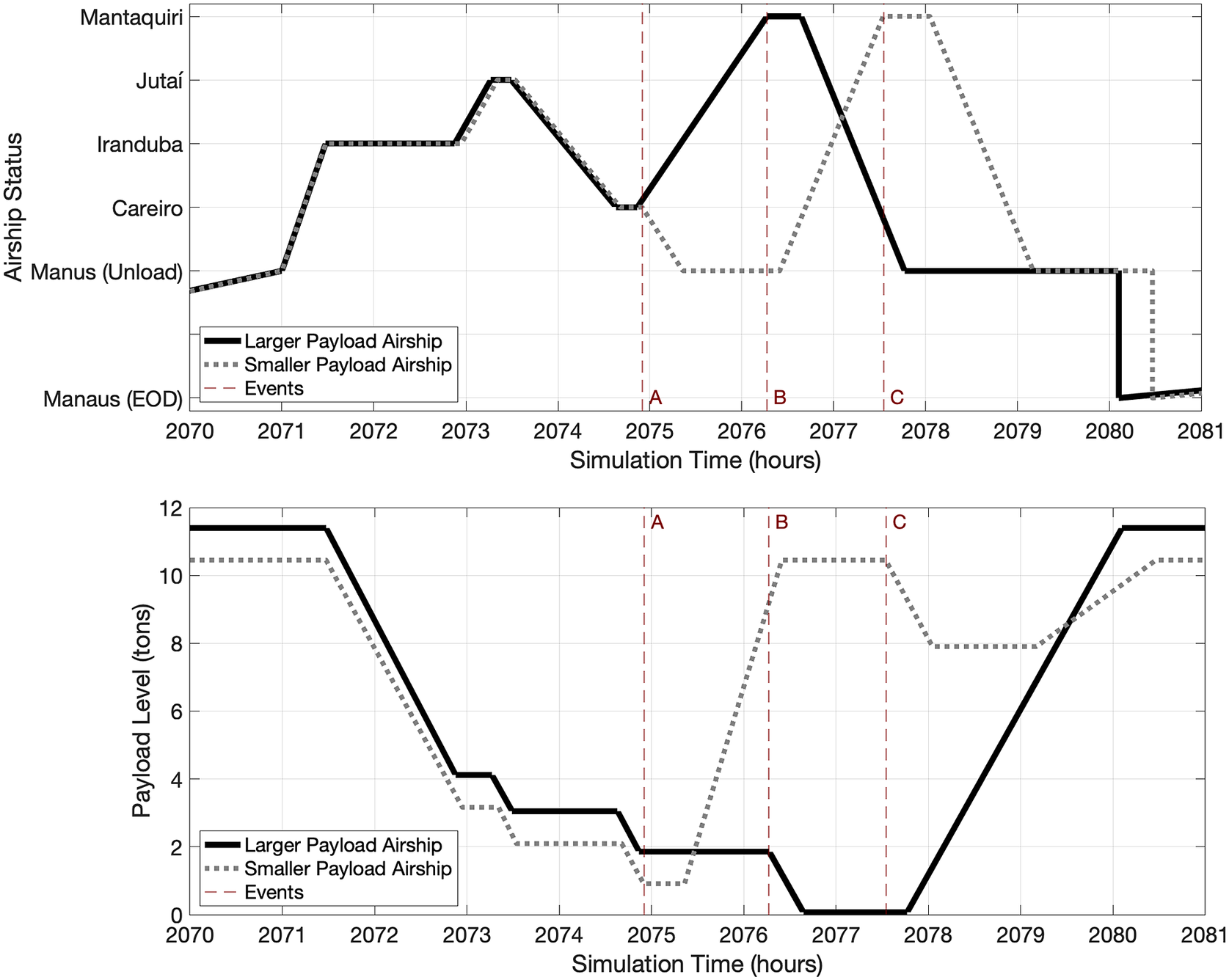
Figure 13. Shown is one day’s activity for two airship designs differing only by a payload of one ton. The airships follow a similar schedule until hour 2075 (denoted by vertical line, Event A). The smaller airship is also unable to visit the fourth city before returning to the hub to unload its cargo. The larger airship loads only a small amount of fruit from the fourth city (Event B). The smaller airship is ultimately able to transport more fruit due to a more productive trip to the fourth city after unloading first in Manaus (Event C).
Additionally, the city decision logic resulted in different routes depending on the system configuration. When airship payloads were low or with fleets of four airships, the resulting routes were hub-and-spoke, favoring the city with the most available fruit (see left-side illustration in Figure 14). As payloads increased, the fleets were able to visit additional cities before returning to unload (see center illustration in Figure 14). When payloads allowed for visiting multiple cities, the routes became more random (see right-side illustration in Figure 14). Had routes been constrained to a certain type of logistics model such as hub-and-spoke or pre-defined, city-to-city circuits based on payload and fleet size, results would have turned out differently.

Figure 14. Depending on the system configuration, the routes taken by the fleets can vary considerably. The diagrams above are three points on the spectrum of possible route options. The weight of the arrows indicate more trips traversing that leg. The return legs are shown as dashed red lines.
The decision of which cities to visit and in which order to visit those cities is complex due to the relationship between airship fleet parameters, city parameters, and the logic of the decision-making algorithm, which included the load threshold parameter. Further exploration in this area would include the addition of an algorithm to the simulation that attempts to solve the traveling salesman problem inherent in the freight transportation domain to find an optimal schedule for each system configuration. But this was beyond the scope of this paper and would add significant computational complexity which could result in each simulation taking orders of magnitude longer. While likely more accurate, it may be less useful as a concept development tool. So while these models and the simulation are not perfect, the simulation of each design took between a thousandth and hundredth of a second to run, general trends of social impact were extracted, and surrogate models were created to find potentially optimal designs.
5.2. Optimization
Using the data generated from the simulations and shown in Figure 9, surrogate models for each impact were created using the neural network predictive modeling tool in JMP Pro, a statistical software by SAS. Each impact was modeled using a two-layer neural network, with each layer consisting of four hidden nodes represented by hyperbolic tangent activation functions. Models were trained on 50% of the data using a hold-back method internal to JMP for the validation on the other half of the data. A squared penalty method and a learning rate of 0.1 were used to train the models. The fit metrics for each model are shown in Table 3.
Table 3. Results of neural network model fitting

The surrogate models of these five impacts were used to find the airship system configuration with the maximum positive impact and minimum negative impact. To do this, the genetic algorithm from Matlab’s Global Optimization Toolbox was used to find the optimum of the cost function:
 $$ O={w}_b{I}_{bn}-{w}_c{I}_{cn}+{w}_f{I}_{fn}-{w}_i{I}_{in}-{w}_t{I}_{tn} $$
where
 $ w $
are weights and
$ w $
are weights and
 $ I $
are normalized versions of the impacts described in Equations 3–7. The subscript
$ I $
are normalized versions of the impacts described in Equations 3–7. The subscript
 $ b $
refers to impact to boat job loss,
$ b $
refers to impact to boat job loss,
 $ c $
refers to the impact to crop savings,
$ c $
refers to the impact to crop savings,
 $ f $
refers to the impact to forest loss,
$ f $
refers to the impact to forest loss,
 $ i $
refers to the impact to farmer income, and
$ i $
refers to the impact to farmer income, and
 $ t $
refers to the impact to farmer time savings. The optimization was performed subject to bound constraints that matched the design variable ranges defined in Table 2 and that also defined the bounds of the DES. Here, the impact to forest was added to act as an additional optimization criterion to ensure that airship designs did not maximize impact for farmers and boat workers at the expense of other rainforest inhabitants, the environment, or others effected by deforestation. Since this simulation took place in the Amazon forest, size could also be limited by available landing area. A 20-ton-carrying airship may be the largest feasible airship for the area if the largest available landing sites are the size of a football pitch. The density and rapid growth of the vegetation in the Amazon make it difficult to clear land. Even if the land is cleared, the forest continually tries to reclaim the land, making it costly to maintain.
$ t $
refers to the impact to farmer time savings. The optimization was performed subject to bound constraints that matched the design variable ranges defined in Table 2 and that also defined the bounds of the DES. Here, the impact to forest was added to act as an additional optimization criterion to ensure that airship designs did not maximize impact for farmers and boat workers at the expense of other rainforest inhabitants, the environment, or others effected by deforestation. Since this simulation took place in the Amazon forest, size could also be limited by available landing area. A 20-ton-carrying airship may be the largest feasible airship for the area if the largest available landing sites are the size of a football pitch. The density and rapid growth of the vegetation in the Amazon make it difficult to clear land. Even if the land is cleared, the forest continually tries to reclaim the land, making it costly to maintain.
As shown in Table 4, the optimization resulted in a different system design depending on the weights. In practice, the weights are dependent on stakeholder preferences. If the stakeholders show no preference to any particular impact, the weights may be equal. This results in a fleet of three airships with one-ton payloads, that travel at 68 knots, and only visit a city if there is one ton of produce available for transport. This design results in less time savings for the farmers, but fewer boat workers must look for new work and very little forest loss may occur. If stakeholders are confident there is enough demand for boat workers elsewhere, they may not consider the impact to boat jobs in their weighting. This results in designs with smaller fleets of larger airships that are capable of transporting all the fruit produced by the four cities while also increasing income for the farmers.
Table 4. Results of optimization using various weightings corresponding to potential stakeholder preferences

Note: First, an equal weighting and has a circle marker. Second, the weighting only shows minor regard for boat job loss and forest loss with an otherwise equal weighting and has a diamond marker. Third, the weighting with a square marker does not consider boat job loss or forest loss and has an otherwise equal weighting. Fourth, equal weight is given to income and time savings, with no regard for other impacts. This weighting has a triangle marker.
These optimal designs are overlaid on the contour plots for each of the four social impacts in Figure 15. The design marked with a square, for example, shows that when boat job loss is no longer a factor, and the importance of forest loss decreases, the design increases in positive impact to income, time savings, and crop loss but in return also increases impact to boat job loss and slightly increases impact to forest loss.

Figure 15. The contour plots of each impact are shown with optimal designs described in Table 4. These points, with markers defined in the bottom, right, show the tradeoffs for each impact to achieve the desired objectives of each cost function weighting. The color scale denotes desirability with green indicating most desirable and pink least desirable.
5.2.1. Operational cost and time
The design obtained from minimizing the cost function where forest loss and boat job loss have decreased priority (diamond symbol in Table 4 and Figure 15), which we will call the optimal-impact design moving forward, may balance the tradeoffs between the social and environmental impacts of interest, but this may be in conflict with other metrics that stakeholders may normally consider such as airship utilization, time to complete the objective, revenue, or cost per ton. The larger airships and larger fleets with higher speeds are able to transport all of the produce quicker than the optimal-impact design. These bigger, faster fleets would also have lower utilization so the airships could then be used by other cities or used for another purpose (see Figure 16). Increasing payload and decreasing fleet size from the optimal-impact design result in designs with lower costs per ton of fruit transported due to the lower fleet acquisition costs and lower helium refill costs throughout the year. Keeping the cruise speed low keeps fuel consumption low contributing to the lower operating costs.

Figure 16. Fleet utilization as a function of airship payload, with cruise speed and load threshold held constant (left), and of cruise speed, with payload and load threshold held constant (right).
The optimal-impact design has a utilization fraction of 0.25, meaning that the airship fleet is being used for 25% of the day, on average, throughout the year. The Pareto-optimal designs for this measure range from 0.35, if a 20-ton airship is traveling around 25 knots, to about 0.12 for fleets traveling above 80 knots and that contain four airships that can carry over 10 tons (see Figure 16). It makes sense that the optimal-impact design is on the higher side of this Pareto-curve as it means the airship is using a high percentage of the allotted time so the fleet is neither working over time nor being significantly underutilized and sitting at the hangar in Manaus for a large portion of the day.
These high-utilization, low time-to-complete designs are also some of the most expensive fleets to operate. The Pareto frontier created by these two competing variables is shown in Figure 17. The configuration that balances cost-per-ton and time-to-complete and the designs at the knee of the curve are four- to seven-ton airships traveling between 45 ando 75 knots in fleets of two airships. Since the optimal-impact design is dependent on many other factors, especially the concern for boat workers and their jobs, the optimal-impact design is not similar to the design that is optimal with respect to time and cost as shown in Table 5.

Figure 17. Fleet utilization and operational cost per ton. Lower utilization means the airship transports all of the produce more quickly, but this is more costly. Lower utilization may also mean that the fleet’s freight transportation capacity is over-designed for the given scenario.
Table 5. Shown is the design optimized for time and cost and the optimal-impact design

Note: The variation in preferences from performance based to impact based results in different designs.
5.2.2. Load rate sensitivity
The simulation is dependent on the rate at which cargo can be loaded onto the airships at each city. The design parameter for this within the simulation was average load rate. This was defined as the time needed to load one ton of cargo onto the airship. The load time was then the product of the tonnage of cargo and a load rate randomly generated from a normal distribution with average load rate as the mean with a standard distribution of 0.01. In the simulations used for this optimization, the average load rate was set to 0.2 hours per ton. Because the load rate directly effects the time each trip takes, optimal designs are likely influenced by the rate at which fruit is loaded onto the airships. Additional simulations were ran for load rates of 0.1–0.5 hours per ton with increments of 0.1 to help determine the sensitivity of the optimal design to this variable. Each of these simulations was ran with a constant load threshold of one ton to match the optimal design from the equally weighted cost function.
The results contained in Table 6 show that load rate indeed affects the optimal airship design. At faster rates, the optimal-impact design consisted of one airship. The jump from 0.1 to 0.2 hours per ton required a larger, faster airship but still only required one of these in the fleet. At 0.3 hours per ton, the slower rate led to the need for two smaller airships to achieve the optimal impact. For system designers, this introduces the decision of whether to spend more on an airship fleet (load rates between 0.3 and 0.5) or to invest more into optimizing the loading process by hiring more workers or introducing more technology.
Table 6. Results of optimization using a range of average load rates and a constant load threshold of one ton

Note: The load rate of 0.2 is the value used in the original optimization.
Further extensions may also include adding additional cities or altering the production schedule or the goods are being produced. The production schedule used in this case study changes drastically through the year and has one city that has much higher production throughout the year than the rest of the cities. A more constant production rate or freight that is more evenly distributed between the cities may have a significant effect on which airship system designs are optimal. The fruit being transported in this example has a very low unit weight relative to the airship payloads. As a result, the cargo can easily be divided into random, small amounts. Other cargo such as fruit processing equipment, wind turbine blades, or other large, indivisible objects would alter how the airship is used since it may be able to carry more weight but not have any space for it, or it may have space for more cargo, but not enough lift.
6. Conclusion
Through the proposed methodology and case study of airship fruit transport in Brazil, we have shown how social impact metrics can be calculated for large-scale products operating within socio-technical systems. We found that by varying airship parameters, it is possible to explore the design space and determine high-potential designs in the context of social impact. By doing so, we provide a possible methodology for other designers of large-scale, shared products operating within socio-technical systems to start from to include social impacts in the system design process.
Going through the process to model and predict the social impact of the airship, we found that the social impact of the airship is highly dependent on the airship-farmer system in addition to the airship’s engineering parameters. We also found that the designs that optimized for product impact were not the same designs that were found optimizing for conventional variables like mission completion time and operational costs per ton transported (see Table 5). Because of this, it is even more important for the system designers and other stakeholders making design decisions to consciously consider social impact as it may not be closely connected to other system requirements related to the problem the product is addressing. This may take the form of including other stakeholders, such as the farmers in the provided case study, in the design process in other ways than solely providing the data that informed the model creation. These stakeholders could provide insights into simulation results and analysis by providing additional information on their preferences with respect to tradeoffs.
Through this process, the importance of the system and operational models to the social impacts became clear. The decisions of farmers and the ways in which the airship was used can have a large influence on the social impacts. This provides the opportunity for further research into the design space of social impacts and engineering parameters. Additionally, this provides the opportunity to further explore how the integration of variable operational and logistic parameters in the simulation can provide further resolution into the calculation of social impact metrics.
There are limitations to the social impacts that could be modeled using the method introduced in this paper. Each of the social impacts predicted in the example is easily quantifiable, while many other social impacts are inherently qualitative. Future work could be done to include qualitative impacts using a mixed-methods approach.
Additional research and refinements to this initial study would generate other findings that could help airship designers and decision-makers maximize the positive social benefit to the area. For example, the surfaces in Figure 9 show the interaction of the product’s sustainability space (Mattson et al. Reference Mattson, Pack, Lofthouse and Bhamra2019) and design space. Applying this linked space, stakeholders could visualize, explore, and better understand the direct interactions between engineering parameters and social impacts. Further investigations into this sustainability-design space could be leveraged to predict the impacts of related airship designs or of other products on society.
What is more, this model only analyzed airships with useful payloads up to 30 imperial tons (13,608 kg) and a variable route between Manaus and each city of farmers. Given different operational parameters such as a different fruit production schedule or city selection criteria, or even a different operational environment all together, the effects to social impact may change considerably with the use-case. Further analysis could also compare different logistics models. Varying the logistical parameters and logic may require additional performance metrics to enable comparison across models. This comparison would determine the optimal combination of airship design for given logistics methods, likely weighing the variations of upfront and operational costs for different numbers and sizes of airships. These interactions may lead to increased social impact metrics that remove or raise the level of the optimal impact. The variation of operational and logistic parameters, if included in the social impact model, could provide further insight into the effects they have on the model and resulting social impact metrics. It may also provide insight on how changes to how the airship is used may provide increased benefit compared to the initial plans for operation.


 Open access