


1. Introduction
With the rapid increases in computational power over the last fifty years, it has become feasible to further understand the three-dimensional features of turbulent flows by resolving numerically the Navier–Stokes and continuity equations using direct numerical simulations (DNS). The DNS data sets obtained from the pioneering simulations by Kim, Moin & Moser (Reference Kim, Moin and Moser1987) and Eggels et al. (Reference Eggels, Unger, Weiss, Westerweel, Adrian, Friedrich and Nieuwstadt1994) demonstrated that the flow statistics obtained from volumetric DNS data sets agree well with existing experimental databases. These numerical experiments have provided extremely useful insights and have advanced our understanding of the physics of steady wall-bounded turbulent flows, such as their statistical universality, scaling laws, flow organisation, self-sustaining process and invariant solutions. Although understanding steady turbulent flows is of significant importance from a fundamental and technological perspective, it is also essential to understand the nature of unsteady turbulent flows with the same depth. However, the physics of unsteady turbulent flows have received relatively little attention by comparison.
Unsteady turbulent flows can be subdivided into two kinds: periodic pulsating flows and non-periodic flows (He & Jackson Reference He and Jackson2000). The former has been studied in more depth, motivated by the nature of biological flows. On the other hand, minimal literature exists regarding the fundamental physics of non-periodic accelerating and decelerating flows. During the last twenty years, only a handful of experimental and numerical investigations have been conducted to investigate the physics of linearly accelerating and decelerating flows. These efforts have mainly focused on the physics and transitional statistics of accelerating turbulent flows. Consequently, it has been possible to understand and obtain a proper characterisation of the transient behaviour of accelerating internal canonical flows (i.e. channel and pipe flows) (He & Seddighi Reference He and Seddighi2013; Guerrero, Lambert & Chin Reference Guerrero, Lambert and Chin2021). Decelerating turbulent flows have received much less attention than accelerating flows. As a result, the literature dedicated to understanding the fundamental physics of decelerating turbulent flows is extremely limited. Thus, the present investigation aims to analyse the transient physics of turbulent pipe flows undergoing a rapid ramp-down reduction in their flow rate using a series of DNS data sets.
1.1. Accelerating turbulent flow
Contrary to intuition, it has been demonstrated that as a fully developed turbulent flow is linearly accelerated, there exists a phase lag in its turbulence response. This implies that if an already turbulent flow is rapidly accelerated, its turbulence kinetic energy (TKE) remains frozen during a relatively short period. In that sense, the seminal study conducted by Maruyama, Kuribayashi & Mizushina (Reference Maruyama, Kuribayashi and Mizushina1976) revealed that there exist two delays associated with the generation of turbulence in a step-up accelerating flow. The first delay is related to the production of ‘new’ turbulence. The second delay is associated with the wall-normal diffusion of the vorticity produced as a result of the acceleration imposed on an already turbulent base flow. Consequently, the time scales associated with the turbulence generation and diffusion in an accelerating flow have been shown to be much larger than the ramp-up time.
To complement and extend the work mentioned above, He & Jackson (Reference He and Jackson2000) carried out a series of ramp-up accelerating flow experiments in a turbulent pipe and obtained three-dimensional measurements of the flow by using a three-beam laser-Doppler velocimeter (LDV). The results of that investigation showed that aside from the two delays observed by Maruyama et al. (Reference Maruyama, Kuribayashi and Mizushina1976), there exists a third delay associated with the redistribution of turbulent kinetic energy amongst the three orthogonal velocity components. Later, Greenblatt & Moss (Reference Greenblatt and Moss2004) gathered time series data sets of rapidly accelerating pipe flows by using single-component LDV. The results from that study revealed that some integral quantities such as the momentum thickness and the displacement thickness exhibited coherence in their time development and showed that a rapidly accelerating turbulent pipe flow followed three transient phases. Jung & Chung (Reference Jung and Chung2012) emulated the experiments conducted by He & Jackson (Reference He and Jackson2000) using large-eddy simulation (LES) data sets. As expected, the results obtained from those simulations confirmed the three-phase lags in the turbulence response observed in the former study (He & Jackson Reference He and Jackson2000).
During the last ten years, special attention has been paid to the time response of the frictional drag in accelerating turbulent pipe and channel flows (He, Ariyaratne & Vardy Reference He, Ariyaratne and Vardy2011). In that regard, several numerical studies have been performed (He & Seddighi Reference He and Seddighi2013, Reference He and Seddighi2015; He, Seddighi & He Reference He, Seddighi and He2016; Jung & Kim Reference Jung and Kim2017; Mathur et al. Reference Mathur, Gorji, He, Seddighi, Vardy, O'Donoghue and Pokrajac2018). The detailed study conducted by He & Seddighi (Reference He and Seddighi2013) analysed the temporal dependence of the mean skin friction coefficient  $C_f$ together with other mean flow statistics to determine the stages undergone by a turbulent channel flow following a step-up increase in the flow rate, using DNS data sets. The results of that study showed that
  $C_f(t)$ in a rapidly accelerating turbulent channel flow exhibits similarities to the bypass transition of a turbulent boundary layer. Additionally, it was concluded that a rapidly accelerating channel flow follows two transient stages, namely pre-transition and transition. The pre-transition phase seems to be associated with the development of a perturbation boundary layer, resulting from a plug-like inflow into the turbulent base flow, whose turbulence is initially frozen. As a result, a decay in the skin friction coefficient is observed. Subsequently,
  $C_f$ attains a minimum; this is nominally the instant at which the pre-transitional period ends and the transitional stage begins. The skin friction coefficient recovers within the transition stage due to the generation of ‘new’ turbulent spots that grow, merge and propagate throughout the flow domain. As the flow fully develops, a plateau in
  $C_f$ is attained.
A recent study conducted by Guerrero et al. (Reference Guerrero, Lambert and Chin2021) investigated the transient flow dynamics of a series of rapidly accelerating turbulent pipe flows between two steady Reynolds numbers ( $Re$) using a series of DNS data sets. That investigation consolidated and extended the different conceptual views existing in the literature (see Greenblatt & Moss Reference Greenblatt and Moss2004; He & Seddighi Reference He and Seddighi2013). The time evolution of the mean flow dynamics of that study exhibited coherence and showed that a rapidly accelerated internal flow follows four transient stages; inertial (stage I), a rapid increase in the viscous forces and a frozen turbulent behaviour; pre-transition (stage II), a weak turbulence response in the near-wall region together with a rapid attenuation in the viscous forces; transition (stage III), a proportional increase in viscous and turbulent forces at the inner region; and core relaxation (stage IV), a slow propagation of turbulence from the wall towards the wake region.
1.2. Decelerating turbulent flow
As mentioned above, non-periodic decelerating flows have received marginal attention compared with the other unsteady flows (i.e. periodic pulsating and non-periodic accelerating flows). The very few experimental studies on this particular topic have reported that as a pipe flow is decelerated, the mean velocity profile at the logarithmic and wake region of the flow is progressively shifted to a lower value during the early flow excursion (Kurokawa & Morikawa Reference Kurokawa and Morikawa1986). However, it maintains the same shape as the initial turbulent base flow within the outer region of the flow. This behaviour in the mean velocity profile has been confirmed from more recent numerical results using Reynolds-averaged Navier–Stokes (Ariyaratne, He & Vardy Reference Ariyaratne, He and Vardy2010) and DNS (Chung Reference Chung2005; Lee et al. Reference Lee, Jung, Lee and Kim2018) approaches.
Following those lines, the DNS study conducted by Mathur (Reference Mathur2016) on decelerating turbulent channel flows revealed that during the early flow excursion there exists the development of a perturbation boundary layer with a negative sign. This perturbation boundary layer exhibits strong similarities with the perturbation velocity profile observed during the early flow excursion in accelerating internal flows (He & Seddighi Reference He and Seddighi2015). It has also been observed that the perturbation boundary layer growth can be modelled using the solution to Stokes’ first problem (He & Seddighi Reference He and Seddighi2015; Joel Sundstrom & Cervantes Reference Joel Sundstrom and Cervantes2017; Mathur et al. Reference Mathur, Gorji, He, Seddighi, Vardy, O'Donoghue and Pokrajac2018). This laminar similarity during the early transient process in accelerating and decelerating flows was confirmed numerically by Mathur (Reference Mathur2016) and experimentally by Joel Sundstrom & Cervantes (Reference Joel Sundstrom and Cervantes2018).
Similar to accelerating flows, the literature has shown that decelerating flows experience a ‘frozen’ turbulence behaviour during the early flow excursion (Maruyama et al. Reference Maruyama, Kuribayashi and Mizushina1976; Ariyaratne et al. Reference Ariyaratne, He and Vardy2010). The same experimental study conducted by Maruyama et al. (Reference Maruyama, Kuribayashi and Mizushina1976) suggests that after the initial ‘frozen turbulence’ period, the TKE follows a somewhat linear decay rate. Along these lines, recent DNS studies of a decelerating turbulent channel flow at low initial Reynolds numbers have revealed that as a flow is decelerated, there exists an anisotropy in the early response amongst the three normal components of the Reynolds stress tensor (Seddighi, He & Orlandi Reference Seddighi, He and Orlandi2011). Moreover, by analysing the time series of the mean friction velocity  $u_\tau (t)$ and the mean centreline velocity
  $\left \langle U_{c}\right \rangle$, Chung (Reference Chung2005) suggested that a decelerating flow follows two transient stages, which exhibited a fast and slow time response, respectively. Nevertheless, the mechanics underlying these two different relaxation periods is not explained in that investigation. More recently, Joel Sundstrom & Cervantes (Reference Joel Sundstrom and Cervantes2018) decomposed the TKE production budget into three components and compared their behaviour between accelerating and decelerating flows, concluding that the turbulence establishment between these two unsteady flows is substantially different.
The temporal evolution of the mean skin friction coefficient and the near-wall dynamics associated with a temporally decelerating internal flow have been analysed in very few studies, and most of them only analyse the frictional drag during the ramp-down period (Shuy Reference Shuy1996; Ariyaratne et al. Reference Ariyaratne, He and Vardy2010; Seddighi et al. Reference Seddighi, He and Orlandi2011) and not during the entire transient process (i.e. until the flow fully develops to its final steady conditions). Indeed, to the knowledge of the present authors, there only exist very few DNS studies that have attempted to examine the transient frictional drag in decelerating internal flows (Chung Reference Chung2005; Mathur Reference Mathur2016; Guerrero, Lambert & Chin Reference Guerrero, Lambert and Chin2022), and in all those cases, the studies were conducted at low  $Re$ turbulence.
From an industrial perspective, most modern fluid transportation systems through pipes are not steady. For instance, the fluid flow through pipes in industrial and domestic facilities is continuously modulated by control valves or pumps to fulfil a specific demand. Nonetheless, due to the lack of knowledge of unsteady flows’ behaviour, the transient effects in these flows are often ignored in the engineering design calculations. As a result, there exist very few reliable unsteady friction models able to predict the frictional drag in accelerating and decelerating turbulent pipe flows.
1.3. Motivation
Most efforts devoted to understanding the physics of temporally decelerating turbulent internal flows have only reported the evolution of mean flow statistics during the ramp-down time. As a result, the complete transient process undergone by a rapidly decelerating turbulent flow has not been analysed thoroughly. Indeed, the very recent textbook by Ciofalo (Reference Ciofalo2022), which devotes a chapter to the analysis of unsteady (periodic and non-periodic) flows explicitly states, ‘The influence of temporal acceleration on turbulence is a different and more subtle issue, which (in the author's opinion) has not found in the literature a really satisfactory treatment so far’. Similarly, the study conducted by Mathur (Reference Mathur2016) in the context of a decelerating turbulent channel flow mentions that ‘…the transition mechanism and timings of the different transitional stages are unclear, possibly due to the masking effect by the existing flow structures at the beginning of the transient or due to the step-down size chosen’. In contrast with the studies associated with the behaviour of rapidly accelerating flows (see Greenblatt & Moss Reference Greenblatt and Moss2004; He & Seddighi Reference He and Seddighi2013; Guerrero et al. Reference Guerrero, Lambert and Chin2021), the different transient stages undergone by a rapidly decelerating flow are still elusive.
As a result, this investigation aims to analyse over a long time scale the transient flow kinematics, dynamics and turbulence decay process associated with a turbulent smooth pipe flow following a rapid temporal ramp-down change in the Reynolds number from one steady flow condition to another. A series of DNS data sets of linearly decelerating turbulent pipe flows with a high spatiotemporal resolution have been conducted for this purpose. Several flow visualisations and high- and low-order one-dimensional and two-dimensional flow statistics have been carefully examined to properly characterise the transient stages experienced by this kind of unsteady flow. It is noteworthy that this investigation does not cover all the features inherent to each of the transient stages experienced by a decelerating wall flow. Instead, this study sheds light on the general dynamics and kinematics that characterise this kind of flow.
2. Numerical details
A series of DNS, using the spectral Navier–Stokes solver Nek5000 (Fischer, Lottes & Kerkemeier Reference Fischer, Lottes and Kerkemeier2019), were performed to gather volumetric time series of resolved flow fields between two steady Reynolds numbers. The spatial domain was a circular pipe whose spectral elements were based on seventh-order Gauss–Lobatto–Legendre quadrature points. Periodic boundary conditions were imposed at both extremes of the pipe. The flow fields were integrated in time using a third-order backward difference scheme. Fully developed turbulent flow fields at an initial steady bulk Reynolds number ( $Re_{b,0} = U_{b,0} D /\nu$) were used as the initial condition. Here,
  $U_{b,0}$ stands for the initial bulk velocity of the flow,
  $D=2R$ is the pipe diameter,
  $R$ is the pipe radius and
  $\nu$ is the kinematic viscosity of the fluid. It should be mentioned that the flow ran for five turnarounds throughout the domain, maintaining the initial steady Reynolds number
  $Re_{b,0}$ in order to attain fully developed turbulence and converged flow statistics before a negative acceleration (i.e.
  ${\rm d}U_b / {\rm d}t < 0$) was imposed. Subsequently, at time
  $t=0$ the flow rate was linearly reduced until it attained a final bulk Reynolds number (
 $Re_{b,1}$). Thereafter, the flow rate was kept constant until the flow fully developed and the universal laws of turbulence converged.
For generality and to properly characterise the transient stages of a rapidly decelerating flow, three different simulation cases were conducted to consider different initial/final Reynolds numbers and deceleration rates. It is noteworthy that each simulation was repeated three times using uncorrelated flow fields as the restarting base flow to obtain convergent flow statistics at each time step. In all cases, the volumetric flow realisations were stored with a time frequency  $t^{+1} \approx 0.5\unicode{x2013}1.0$ to track the time evolution of the different flow quantities adequately. The general set-up of each simulation is summarised in table 1. Additionally, the reader is referred to figure 1(a) to visualise the ramp-down change imposed in the Reynolds number.

Figure 1. (a) Ramp-down change in the bulk Reynolds number  $Re_b$ for the present cases D1 (
![]() ), D2 (
), D2 ( $- ~ - ~ - ~ -$) and D3 (
 $- {\cdot } - {\cdot } -$). Case D3 is compared with the channel flow DNS by Mathur (Reference Mathur2016) (
 $\circ$). (b) Transient response of the skin friction coefficient for the cases depicted in (a).
Table 1. Computational parameters used in the numerical simulations. The ‘ $+$’ superscript denotes normalisation in viscous units, and the ‘0’ and ‘1’ indices denote the initial and final steady states. The subscripts ‘ramp’ and ‘samp’ stand for the acceleration time and the sampling time intervals at which three-dimensional flow realisations have been stored. The variable
  $\gamma = [{\rm d}U_b/{\rm d}t\,D/(U_{b,0} u_{\tau,0})]$ is the dimensionless ramp-rate parameter proposed by He & Jackson (Reference He and Jackson2000).

Due to the nature of a straight and smooth pipe, a cylindrical coordinate system has been adopted in this paper, where  $r$,
$r$,  $\theta$ and
  $z$ are the radial, azimuthal and streamwise directions, respectively. The wall-normal direction is denoted as
  $y=R-r$. Similarly, the resolved flow fields contain three orthogonal velocity components
  $U_r = -Uy$,
  $U_\theta$ and
  $U_z$ whose fluctuating components are
  $u_r=-u_y$,
  $u_\theta$ and
  $u_z$. Note that the ‘
 $+0$’ or ‘
 $+1$’ superscripts denote normalisation in viscous units at the initial or final steady Reynolds numbers of the simulations, respectively. Herein, the viscous unit length is
  $\delta _\nu = \nu /u_\tau$, where
  $\nu$ is the kinematic viscosity of the fluid. The friction velocity is defined as
  $u_\tau = \sqrt {\left \langle \tau _w\right \rangle /\rho }$, where
  $\left \langle \tau _w \right \rangle$ is the ensemble mean wall shear stress and
  $\rho$ is the fluid density. The ensemble average of any fluid quantity will be denoted using angle brackets within the present investigation. For instance, the ensemble-averaged streamwise velocity normalised in viscous units using the final steady friction velocity will be denoted as
  $\left \langle U_z\right \rangle ^{+1}=\left \langle U_z\right \rangle /u_{\tau,1}$.
3. Near-wall behaviour and flow structures
3.1. Response in the mean skin friction coefficient
The time dependence in the bulk Reynolds number  $Re_b(t)$, as a result of imposing a rapid ramp-down reduction in the flow rate in all the cases analysed in this study, is observed in figure 1(a). As explained previously, at
  $t^{+1} < 0$ the flow remained at a stationary Reynolds number
  $Re_{b,0}$. Later, at
  $t^{+1}=0$ a ramp down in the flow rate was imposed to reduce the Reynolds number rapidly. Once the final Reynolds number (
 $Re_{b,1}$) is attained, the flow rate remains constant until the vorticity (
 ${\pmb {\omega }}$) is attenuated across the entire pipe domain, the flow fully develops and a quasi-steady behaviour is obtained in the different flow statistics analysed in this study.
The temporal response in the mean skin friction coefficient (i.e.  $C_f = \tau _w/(0.5\rho U_b^2)$) for cases D1, D2, D3 and the benchmark channel flow data from Mathur (Reference Mathur2016) are displayed in figure 1(b). In general, it can be observed that the skin friction coefficient presents coherence in its behaviour. Additionally, its time response suggests that the flow experiences several transient stages before attaining a stationary behaviour. Aside from the mean skin friction coefficient response, the different stages have been heuristically characterised by analysing the different flow statistics presented throughout this paper. Our results suggest that similar to an accelerating turbulent flow, a decelerating flow exhibits four unambiguous transitional stages as follows.
(i) Stage I: during the early flow excursion, there exists a quick and nonlinear decay in the skin friction coefficient. This rapid decay is related to a sudden adverse pressure gradient imposed in the flow. As a result, a plug-like reduction in the mean velocity profile occurs during this early stage, as will be shown later. It is interesting to note that case D1 attains negative values in
 $C_f$ during this stage. This implies that flow separation exists at the near-wall region (i.e. there are reverse flows near the wall, leading to an inflectional velocity profile), consistent with the temporal adverse pressure gradient imposed to reduce the flow rate. Additionally, the fact that $C_f$ attains negative values implies that the mean wall shear stress has negative values ($\left \langle \tau _w\right \rangle < 0$) during the early flow excursion. Consequently, the instantaneous friction velocity ($u_\tau (t) = \sqrt {\left \langle \tau _w\right \rangle /\rho }$) is not a suitable scaling argument during this period since it would be an imaginary variable.
(ii) Stage II: as the flow excursion stops (i.e. the flow rate remains constant),
$C_f$ experiences a rapid recovery and overshoots its final steady-state value.(iii) Stage III: after
$C_f$ attains a maximum, a progressive decay is observed, associated with an attenuation of the turbulent motions. Note that the flow rate has remained constant for a considerable time during this period. However, as explained later, the transient turbulence dynamics require extensive periods to stabilise.(iv) Stage IV: after the
$C_f$ has decayed, it plateaus, suggesting that the flow has developed, at least within the near-wall region. Nevertheless, a constant value in $C_f$ does not necessarily imply that the flow has fully developed throughout the entire domain (Guerrero et al. Reference Guerrero, Lambert and Chin2021). Indeed, the analyses conducted in the following sections indicate that similar to the accelerating case, a decelerating flow also exhibits a core-relaxation period. It is noteworthy that a complete analysis of the time response of several mean flow statistics $f(y,t)$ has been conducted in the following sections to characterise and examine thoroughly the transient stages experienced by a rapidly decelerating flow.


3.2. Flow visualisations
3.2.1. Temporal evolution of the vortical structures
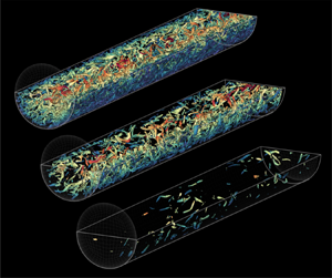
Here, the temporal behaviour of some characteristic flow structures during the transient process of a decelerating flow is analysed. Figure 2 depicts several instantaneous flow visualisations of the vortex cores using the  $\lambda _2$ criterion (Jeong & Hussain Reference Jeong and Hussain1995) at several instants for case D2. In figure 2(a) it is observed that the entire pipe domain, at its initial steady state, is populated with vortical structures extending from the wall towards the pipe centreline. Afterwards, at
  $t^{+1}>0$ the flow excursion takes place. During the early moments of the inertial period or stage I (figure 2b), it is noted that the vortex cores do not exhibit noticeable changes compared with the turbulent base flow. Subsequently, the snapshot obtained during the early stage II (figure 2c) shows that at the end of the ramp-down change imposed in the flow rate there exists a reduction in the population of vortical structures at the near-wall region. This is highlighted within the zoomed insets of figures 2(b) and 2(c). In figure 2(c) it is also noted that the core region of the flow has not undergone substantial changes. This implies that the turbulence decay for a decelerating wall-bounded flow starts at the wall. Subsequently, at
  $t^{+1} \approx 83$ (figure 2d), which coincides with the peak in
  $C_f$ attained in case D2 (i.e. at the onset of stage III), it is noted that the amount of turbulent eddies has been substantially reduced near the wall. Additionally, several void spaces can be observed from the wall up to
  $y/R \approx 0.5$, where turbulence has been attenuated. After
  $t^{+1}>83.4$, a substantial decay in turbulence exists. Furthermore, it is noted that the existing turbulent eddies are progressively annihilated or dampened in the wall-normal direction as time increases. This implies that, similar to the turbulence generation produced in accelerating pipe flows, the attenuation of turbulence in decelerating wall flows occurs at the wall and propagates by diffusion in the wall-normal direction. In figure 2(e), at
  $t^{+1} = 180$, near the end of stage III, it is noted that turbulence has substantially reduced throughout most of the pipe domain. Nevertheless, during stage IV, the core region requires long time scales to relax, as explained in the following sections. Finally, as the flow has fully developed (figure 2 f), it exhibits the behaviour and the characteristic flow structures of low-Reynolds-number turbulence.

Figure 2. Temporal evolution of the vortical structures using the  $\lambda _2$ criterion. The isosurfaces were computed at a level
  $\lambda _2^+ = -0.5$. The snapshots were obtained during the different stages experienced by the decelerating flow: (a) initial steady state, (b) inertial stage or stage I, (c) friction recovery or stage II, (d) turbulence decay or stage III, (e) core relaxation or stage IV and ( f) final steady state.
3.2.2. Temporal evolution of the velocity streaks
It is well known that the turbulent vortices, especially the streamwise rolls, are responsible for generating the characteristic alternating velocity streaks observed in turbulent flows (Kline et al. Reference Kline, Reynolds, Schraub and Runstadler1967). Thus, a wall-parallel plane showing the streamwise velocity fluctuation at  $y^+ \approx 12$ has been computed and is depicted in figure 3 in order to understand how the turbulent streaks respond to a rapid reduction in the flow rate. It should be mentioned that the sequential plots of streamwise fluctuation have been computed for the same flow fields shown previously in figure 2, and the streamwise fluctuation field
  $u_z(t)$ has been normalised with the instantaneous bulk velocity
  $U_b(t)$. The turbulent steady base flow at
  $Re_\tau \approx 340$ is shown in figure 3(a), where the alternating high/low-speed streaks of a turbulent flow at moderate Reynolds numbers can be observed.

Figure 3. Temporal evolution of the velocity streaks at  $y^{+1} = 12$. The streaks have been computed for the same flow realisations exhibited in figure 2(a–f).
A careful examination of the behaviour in the velocity streaks reveals that during the early inertial stage (figure 3b) the streaks have advected in the streamwise direction showing a similar topology as the base flow. Nonetheless, it is possible to see that the magnitude of both high- and low-speed streaks has increased, implying a possible increase in turbulence, at least at the buffer region, throughout this period. Within the same subfigure, it is also observed that even though the low-speed streaks (blue contours) preserve similar length scales to the initial base flow, the sinuosities, characteristic of the turbulent streaks, are amplified. This suggests that the sinuous secondary instability seems to be one of the mechanisms that momentarily enhances turbulence at the buffer region throughout stages I and II, before the turbulence decay occurs. The following sections will further confirm these observations by analysing different flow statistics.
Figure 3(c) reveals that at the end of the inertial period (onset of stage II), the low-speed streaks are substantially different from the structures observed in the turbulent base flow. Indeed, it is noted that the low-speed streaks are wider, its sinuosities have been considerably amplified, and their magnitude is higher than the streaks observed in the turbulent base flow. As a result, the flow at the buffer layer exhibits higher intermittency throughout this period, which is consistent with the growth of the sinuous secondary instability mentioned above. In fact, the recent study of an impulsively decelerating Taylor–Couette flow by Kaiser et al. (Reference Kaiser, Frohnapfel, Ostilla-Mónico, Kriegseis, Rival and Gatti2020) showed that secondary instabilities grow within the near-wall region after the flow is decelerated. This behaviour is consistent with the momentary overshoot of the Reynolds shear stress within the buffer layer observed during stage II, explained in the following sections.
A snapshot obtained at the end of the friction recovery stage (onset of the turbulence decay period) is shown in figure 3(d). Within this flow realisation, it is noted that the streamwise streaks exhibit, qualitatively, a larger scale when compared with the prior snapshots, evidencing a decay in turbulence. Moreover, the low-speed streaks depicted in this flow realisation still exhibit highly sinuous patterns with respect to the fully developed turbulent flow at its final steady state (figure 3 f). Later, at the end of the turbulence decay period (figure 3e), the organisation and structure of the streamwise fluctuation field at the buffer region show substantial similarities with the final steady turbulent state (figure 3 f).
To further analyse the behaviour in the streaks, especially during the inertial (stage I) and early friction recovery (stage II) stages, a series of sequential snapshots between  $0 \leqslant t^{+1} \leqslant 49.6$ have been computed for case D2 and are shown in figures 4(a)–4( f). Within these figures, the blue isosurfaces represent the low-speed streaks computed at
  $u_z/U_b = -0.2$, and the green isosurfaces are the near-wall vortices computed with the
  $\lambda _2$ criterion at a level
  $\lambda _2^{+0} = -3$. It should also be noted that within these snapshots the pipe has been ‘unwrapped’ to provide a clearer view of the low-speed streaks. Figure 4(a) shows the initial steady-state base flow at
  $t^{+1}=0$, which shows the typical configuration of a fully turbulent flow. During the early inertial period (figure 4b), the streaks exhibit a slight growth in the streamwise and wall-normal directions. It is also noted that, during the early flow excursion, the vortical structures’ population, length scales and topology do not exhibit substantial changes.

Figure 4. ‘Unwrapped’ snapshots of case D2 showing the time evolution of the low-speed streaks and vortical structures during the (a–e) inertial (stage I) and ( f) early friction recovery (stage II) periods. The low-speed streaks are depicted in blue isosurfaces and have been computed at a level  $u_z/U_b=-0.2$. The green isosurfaces are the vortical structures computed using the
  $\lambda _2$ criterion at a level
  $\lambda _2^+=-3$.
As time progresses, it is observed that the low-speed streaks continue growing in length and start merging, as shown in figure 4(c,d) (also see figure 5(c,d) for clarity). Moreover, as the streaks grow, amplification in the sinuous mode (secondary instability) and a slight increase in the population of azimuthal vortical structures above the highlighted streaks are noted. It should be mentioned that several flow realisations analysed by the authors (not shown here) reveal that this process seems universal in rapidly decelerating flows. For a more explicit observation of the sinuous instability experienced by the streaks during stage I, zoomed in top views of figures 4(a–f) can be seen in figures 5(a–f).

Figure 5. Temporal evolution of the low-speed streaks during the inertial (stage I) and early friction recovery (stage II) periods. The snapshots are a zoomed top view from figure 4.
At the end of the inertial stage (figures 4e–f and 5e–f), the streaks exhibit elongated patterns in the azimuthal direction, occurring during the merging process. This confirms the change in the topology of the streaks and shows a possible amplification in the secondary instability as noted in figure 3(c). From a structural standpoint, these observations reveal that the behaviour of the low-speed streaks along the inertial and the early friction recovery stages in rapidly decelerating flows are substantially different from the pre-transitional stage of rapidly accelerating flows. It should be recalled that, during the pre-transitional stage of accelerating internal flows, the low-speed streaks elongate in the streamwise direction and temporarily become more stable (He & Seddighi Reference He and Seddighi2013). On the other hand, the present results reveal that throughout stages I (inertial) and II (friction recovery), the sinuous secondary instability is temporarily amplified, the streaks merge and their topology exhibits differences from a fully developed steady turbulent flow. Indeed, during the early friction recovery period, it is possible to observe elongated patterns in the azimuthal direction.
4. Mean flow statistics
The brief analysis conducted from the instantaneous flow visualisations observed in figures 2–5 has provided a qualitative insight into the decay of turbulence and the evolution of the velocity streaks. Nevertheless, conducting a series of statistical analyses is necessary to properly characterise the mean flow dynamics inherent in the transient behaviour of a decelerating turbulent pipe flow. Since the present study focuses on characterising the transient stages experienced by a rapidly decelerating turbulent flow, the volumetric time series obtained from simulation D1 will be used to analyse the transient behaviour undertaken by a decelerating flow from a statistical perspective. It is noteworthy that the present authors have conducted similar analyses for cases D2 and D3 (not shown here), and it has been observed that the flow development at lower  $Re_\tau$ agrees well with the high
  $Re_\tau$ case both quantitatively and qualitatively.
4.1. Time response of the mean velocity profile
Throughout the rest of this study, the flow statistics associated with case D1, whose initial and final steady friction Reynolds number is  $Re_{\tau,0} \approx 830$ and
  $Re_{\tau,1} \approx 500$, respectively, are analysed. This case was chosen as it was conducted at higher initial and final Reynolds numbers.
In order to further understand the temporal response observed in the skin friction coefficient, it is insightful to analyse the temporal evolution of the mean velocity profile. Following the proposed stages undergone by decelerating flows, figures 6(a)–6(d) exhibit the time dependence of the mean velocity profile scaled in viscous units at the final steady Reynolds number ( $Re_{b,1}$) attained by the flow. In figure 6(a) it is noted that during the flow excursion, the mean velocity profile
  $\left \langle U_z\right \rangle ^{+1}$ is shifted downwards without exhibiting substantial changes in its shape within the buffer and the wake regions of the flow (i.e. at
  $y^{+1}>10$). This suggests that there exists a plug-like reduction in the mean velocity profile during the early flow deceleration. This agrees well with the early experimental observations by Maruyama et al. (Reference Maruyama, Kuribayashi and Mizushina1976) and the recent DNS study by Lee et al. (Reference Lee, Jung, Lee and Kim2018). Nevertheless, a careful examination of the near-wall flow provided by the inset exhibited in figure 6(a) shows substantial changes within the viscous sublayer of the flow. Firstly, it should be noted that during this transient stage, the mean velocity profile does not follow the well-known linear behaviour of the viscous sublayer observed in fully developed steady turbulence. Furthermore, at
  $t^{+1} \approx 9$ the existence of a reverse flow region within
  $0 \leqslant y^{+1} \leqslant 2$ is shown. As a result, an inflectional velocity profile is produced, resulting from the temporal adverse pressure gradient imposed to reduce the flow rate. The inflectional velocity profiles tend to be unstable (Drazin & Reid Reference Drazin and Reid2004). Indeed, the generation of an inflectional profile could be both a consequence of the adverse pressure gradient imposed to decelerate the flow, and the temporary amplification of the sinuous secondary instability observed previously in figure 3.

Figure 6. Temporal evolution of the mean velocity profile of case D1 normalised in viscous units with  $\nu$ and
  $u_{\tau,1}$. The plots have been computed during the four transient stages: (
 $a$) inertial (stage I), (
 $b$) friction recovery (stage II), (
 $c$) turbulence decay (stage III) and (
 $d$) core relaxation (stage IV). Here (
 $- {\cdot } -$) is the initial steady state and (
 $---$) the final steady state. The arrows represent increase in time. For the colour legend, refer to figure 8.
During stage II, namely friction recovery (figure 6b), it is observed that  $\left \langle U_z \right \rangle (y,t)$ mainly changes within the near-wall region of the flow (i.e.
  $y^{+1}<30$), and its overlap and wake regions are largely frozen during this stage. The same figure shows that the mean velocity profile progressively shifts upwards within the viscous sublayer. As a result, the velocity gradient at the wall increases throughout this period, which is consistent with the rapid increase observed previously in the skin friction coefficient.
Contrary to the second stage, the turbulence decay period (figure 6c) exhibits a nearly unchanged behaviour within the viscous sublayer. However, during this period, the mean velocity profile presents its most relevant changes within the buffer and overlap regions ( $10 \lesssim y^{+1} \lesssim 100$). It is also noted that, during this stage, the wake region exhibits a marginal change, indicating that decelerating flows possibly have a nearly ‘quiescent’ behaviour at the core region during the three first transitional stages, similar to their accelerating counterpart (Guerrero et al. Reference Guerrero, Lambert and Chin2021). At the end of this stage, the mean velocity profile at the viscous sublayer starts converging, and its characteristic linear behaviour is recovered.
Throughout the fourth stage (core relaxation), the near-wall region  $y^{+1} \lesssim 30$ exhibits convergence as it is nearly unchanged with time. Nevertheless, the mean velocity profile keeps reshaping at the overlap and wake regions. The most substantial changes in the velocity profile seem to occur in the wake of the flow. Precisely, the mean profile at the wake region shifts downwards considerably until it converges with the final steady state at a lower
  $Re_{b,1}$.
4.2. Time response of the flow scales
As a complement to the flow visualisations presented previously in § 3.2.2, here we analyse the time dependence of the two-point correlations  $R_{u_z u_z}$ of the streamwise velocity fluctuation field at a wall-parallel plane located at
  $y^{+1} \approx 12$ in the
  $z$ direction. The two-point correlations allow us to quantify the mean streamwise length of the flow scales throughout the transient process of the decelerating pipe flows analysed in this study. The results exhibited in figure 7(a) reveal that the streaks have an average streamwise length (
 $\Delta z/R \approx 2.8$) during the early inertial stage (
 $0 < t^{+1} \lesssim 5$). Later, a slight increase in the correlation is noted, revealing a minor growth in the average streamwise length of the streaks.

Figure 7. Two-point correlation of the velocity streaks at  $y^{+0} = 12$ computed for case D1 during the four transient stages. Here (
 $- {\cdot } -$) is the initial steady state and (
 $---$) the final steady state. The arrows represent increase in time. The intersection between the vertical lines and the horizontal grey line represents the streamwise length of the streaks correlated at
  $R_{u_zu_z}=0.05$. For the colour legend, refer to figure 8.
The results observed in figure 7(b) reveal that during the friction recovery period, the streaks experience substantial growth in their length. Indeed, at the end of this period, the correlation increases and shows that the maximum average streamwise length attained by the streaks is approximately  $\varDelta _z/R \approx 4.9$. This value represents a 75 % increase in the average length scale of the streaks. Subsequently, during the transitional period (figure 7c), a progressive reduction in the correlation up to
  $\varDelta _z/R \approx 3.7$ is noticed. Finally, figure 7(d) shows that throughout the core-relaxation period, negligible changes exist in the near-wall streaks as the correlation seems to fluctuate around the final stationary value of the flow.
4.3. Time evolution of the Reynolds and viscous shear stresses
Figures 8(a)–8(d) depict the time response in the Reynolds ( $\left \langle u_r u_z \right \rangle ^{+1}$) and viscous (
 $\left \langle - \partial U_z / \partial r\right \rangle ^{+1}$) shear stresses for case D1. During stage I (figure 8a), it is observed that the viscous stress undergoes a substantial reduction within the viscous sublayer and part of the buffer region. It is noted that at
  $t^{+1}\approx 9$ (purple dashed line) the viscous stress at the wall and within the viscous sublayer attains negative values. The
  $(-\partial U_z / \partial r)$ term is the major contributor to the azimuthal vorticity
  $\omega _\theta$ and the mean azimuthal vorticity
  $\left \langle \omega _\theta \right \rangle = \left \langle -\partial U_z / \partial r \right \rangle$. This implies that, on average, a small layer of negative azimuthal vorticity is produced at the wall during the flow excursion. Indeed, in the recent work by Guerrero et al. (Reference Guerrero, Lambert and Chin2022) it was shown that large-scale patches of negative wall shear stress are generated during the early flow excursion in a decelerating flow. It should also be mentioned that vorticity can only be produced at the wall (Batchelor Reference Batchelor1967; Morton Reference Morton1984) due to local accelerations. This implies that negative azimuthal vorticity (i.e.
  $\omega _\theta < 0$) is immediately produced at the wall due to local adverse pressure gradients, and subsequently, this negative vorticity is later transported away from the wall by viscous diffusion. A possible mechanism of vorticity decay in decelerating wall-bounded flows will be analysed later. During this period, it is also noted that the Reynolds shear stress undergoes a mild reduction in its magnitude within the viscous sublayer during the early part of this period. Nevertheless, during the late inertial period, it is noted that
  $\left \langle u_r u_z\right \rangle ^{+1}$ slightly overshoots the initial Reynolds shear stress within
  $10 \lesssim y^{+1} \lesssim 30$, indicating a slight increase in turbulence at the buffer produced by the inflectional profile and sinuous secondary instabilities that grow throughout stages I and II. This is consistent with the observations made from figure 3(b,c). At the core region, an unchanged behaviour in the Reynolds shear stress is noted during this short stage, indicating that turbulence is nearly frozen in most of the flow domain throughout this period.

Figure 8. Temporal evolution of the viscous and Reynolds shear stresses computed for case D1. The flow quantities have been normalised in viscous units with  $u_{\tau,1}^2$. Here (
 $- {\cdot } -$) is the initial steady state, (
 $---$) the final steady state, (solid coloured) Reynolds shear stress and (dashed coloured) viscous shear stress. The arrows represent an increase in time.
Stage II, namely friction recovery (figure 8b), exhibits a quick recovery in the viscous shear stress within the viscous sublayer, and at the end of this stage it overshoots the final steady-state value, which agrees with the peak observed in the time response of the skin friction coefficient throughout this stage. Simultaneously, the viscous stress experiences a progressive reduction within the buffer layer, owing to a possible diffusive mechanism. Hence, it is noted that the viscous shear stress overshoots the final steady state within the viscous sublayer, undershoots the final steady state at the buffer region and remains nearly unchanged at the outer region of the flow. In the same subfigure it is possible to note a progressive decay in the Reynolds shear stress within the inner region of the flow ( $y^{+1}\lesssim 50$). Nonetheless, it is interesting to observe that within the buffer region, before turbulence decays at a particular wall-normal position, the peak value of the instantaneous Reynolds shear stress momentarily overshoots the initial steady-state value followed by a decay in
  $u_ru_z$. Within this stage, the core region exhibits a nearly unchanged behaviour in the Reynolds shear stress, implying that the turbulence decay mechanism generated at the wall requires extensive periods to propagate towards the wake region.
Figure 8(c) shows that during the turbulence decay period there exists a considerable attenuation in turbulence from the wall towards the buffer and overlap regions. This is evidenced by the behaviour observed in the Reynolds shear stress, which exhibits a substantial reduction within the buffer region during the early part of stage III. Thereafter, during the late instants of this period, it is noted that the Reynolds shear stress undergoes a substantial decay within the overlap region up to  $y^{+1} \approx 200$. Additionally,
  $\left \langle u_r u_z\right \rangle$ is nearly unchanged within
  $200 \lesssim y^{+1} \lesssim 500$, showing that during the first three stages, the turbulence decay has only affected approximately 40 % of the flow in the wall-normal direction. Similarly, the viscous stress near the wall exhibits slow decay within the viscous sublayer due to turbulence reduction. However, it is possible to observe that the viscous stress tends to recover within the buffer region and approaches the final steady state.
The fourth stage, core relaxation, is shown in figure 8(d), where it is possible to note that the Reynolds shear stress is nearly unchanged within the near-wall region. However, it exhibits a substantial decay within the overlap and wake regions. It should be noted that the time scales associated with this period are considerably larger than the previous three stages as they are associated with the diffusion of vorticity within the wake region and along the  $y$ direction. This observation agrees with the conceptual view of a ‘quiescent’ core associated with the large-scale uniform momentum zones located within the wake region (Yang, Hwang & Sung Reference Yang, Hwang and Sung2019; Chen, Chung & Minping Reference Chen, Chung and Minping2020). Finally, it is worth mentioning that the viscous shear stress exhibits negligible changes during this period, which is consistent with the plateau attained in
  $C_f$. Similar to the observations in accelerating flows, it is noteworthy that a plateau attained by
  $C_f$ is not necessarily an indication that the flow has fully developed. Indeed, the near-wall flow dynamics is nearly established during this considerably large period. Hence, the near-wall flow statistics may seem unchanged. However, the wake region requires significant time scales to relax as the decay of turbulence requires extensive periods to diffuse within the core region.
4.4. Reynolds shear stress spectra
The pre-multiplied co-spectra  $k \phi ^{+1}_{u_r u_z}$ was computed to extend the analysis of the Reynolds shear stress provided previously. The quantity
  $k \phi ^{+1}_{u_r u_z}$ is a useful tool to understand the scales of motion and the flow regions that undergo turbulence energy growth or decay in an unsteady flow. The result of computing
  $k \phi ^{+1}_{u_r u_z}$ for case D1 during the initial steady state at
  $Re_\tau \approx 830$ is observed in figure 9(a). The transient process during stages I–IV is shown in figures 9(b)–9(e). Finally, the co-spectra of the final steady state at
  $Re_\tau \approx 500$ is observed in figure 9( f). The location and the length scales where the energy decay is produced can be determined qualitatively from figure 9. However, to better understand the length scales and the position where the energy decay occurs, the subtraction between the two consecutive snapshots during the different stages has been computed (i.e.
  $\phi ^{+1}_{u_r u_z}(t+\Delta t) - \phi ^{+1}_{u_r u_z}(t)$). Figure 10 shows the result of that difference. For instance, figure 10(a) shows the result of subtracting figures 9(b) and 9(a).

Figure 9. Temporal evolution of the Reynolds shear stress pre-multiplied co-spectra  $k \phi ^+_{u_r u_z}$ throughout the different stages undergone by the flow: (a) initial steady state, (b) inertial, (c) friction recovery, (d) turbulence decay, (e) core relaxation, ( f) final steady state. The horizontal white dashed line represents the location of
  $\lambda ^{+1}=1000$.

Figure 10. Energy decay in the Reynolds shear stress co-spectra throughout the four transitional stages underwent by case D1. The energy decay at each stage was computed by subtracting two consecutive spectrograms from figures 9(a)–9(e). The horizontal white dashed line represents the location of  $\lambda ^{+1}_z=1000$ and the vertical dashed lines are plotted at
  $y^{+1} = 30$ and
  $y^{+1} = 200$, respectively.
Figure 10(a) shows that during the inertial period there exists a mild energy decay at the near-wall region ( $y^+ < 10$) in wavelengths oscillating between
  $100 \lesssim \lambda ^{+1}_z \lesssim 1000$. Negligible changes in energy growth or decay are observed within the overlap and outer regions of the flow.
The energy growth/decay during the second stage (friction recovery) is depicted in figure 10(b). It is noted that within the inner region of the flow ( $y^{+1}<30$) the energy decays mainly in the small-scale spectrum (
 $\lambda ^{+1}_z < 1000$). However, some wavelengths around
  $1000 \lesssim \lambda ^{+1}_z \lesssim 3000$ undergo an energy decay. At the overlap region (
 $30 \lesssim y^+ \lesssim 200$), energy growth is observed in the small-scale spectrum. This observation is consistent with the slight overshoot in the peak of the Reynolds shear stress observed in figure 8(b). During this period, the wake region does not exhibit significant changes in the spectral energy distribution. This shows that the energy losses due to a flow deceleration start at the near-wall region, and the small-scale motions are the first to respond to this kind of perturbation.
As expected, most of the energy decay in the inner region of the flow occurs throughout the turbulence decay period, or stage III. The energy changes are shown in figure 10(c). This figure reveals a significant energy decay at the buffer and the overlap regions. It is noteworthy that, in this stage, most of the energy decay occurs within the small-scale spectrum. However, a non-negligible contribution in the energy decay happens at the overlap region at large- and very-large-scale wavelengths ( $10^3 \lesssim \lambda ^{+1}_z \lesssim 10^4$). It is also interesting to note that at the wake region there is a mild energy decay in the small scales of motion together with a slight energy growth in the large scales of motion. The reasons for producing this energy decay and growth in the different scales of motion at the same radial location is likely due to the wall-normal propagation of a shear layer (refer back to figure 6).
Finally, the core-relaxation period reveals minor energy losses at the inner region of the flow. As expected, most of the energy losses are observed within the wake region of the flow throughout all the scales of motion. However, due to the nature of the core region, the wavelengths  $\lambda ^{+1}_z \approx 1000$ exhibit the most significant energy losses.
5. Analysis of the flow dynamics and higher-order statistics
5.1. Time dependence of the $u_z u_z$ budgets

The high definition provided by the DNS data sets allows for having highly accurate results in the velocity gradient tensor. As a result, it is possible to analyse the temporal evolution of the Reynolds stress budgets. Here, we will focus on the  $u_z u_z$ budget, which is the major contributor to the TKE budget. The equations derived by Eggels et al. (Reference Eggels, Unger, Weiss, Westerweel, Adrian, Friedrich and Nieuwstadt1994) have been used to compute the
  $u_z u_z$ budget in cylindrical coordinates. The notation adopted in this section is as follows: turbulence production
  $\mathcal {P}$, pressure strain
  ${\varPi }$, viscous dissipation
  ${\epsilon }$, turbulence transport
  $\mathcal {T}$ and viscous diffusion
  $\mathcal {D}$. Similar to the statistical quantities analysed previously, the
  $u_z u_z$ budgets have been normalised with
  $u_{\tau,1}^4/\nu$, and the results are depicted in figures 11(a)–11(d). It should also be noted that the turbulence production, dissipation and pressure strain for the initial steady state have been plotted for reference.

Figure 11. Time evolution of the  $u_z u_z$ budgets for case D1 throughout the four transient stages: (
 $a$) inertial, (
 $b$) friction recovery, (
 $c$) turbulence decay and (
 $d$) core relaxation. For the legend, see (
 $a$).
$a$).
During stage I (figure 11a), it is noted that  $\mathcal {P}^{+1}$ and
  ${\epsilon }^{+1}$ exhibit an early response (decay) within the near-wall region, and an unchanged behaviour at the outer region of the flow. This agrees with the previously presented results regarding the time response of the Reynolds and viscous stresses, where it was observed that the decay of turbulence in a decelerating flow starts at the wall. It is noteworthy that even though
  $\mathcal {P}^{+1}$ and
  ${\epsilon }^{+1}$ show an early response within
  $y^{+1}\lesssim 10$, the pressure strain term remains almost unchanged, even at the near-wall region, during the early flow excursion. Since the pressure strain term acts as a sink term to the Reynolds stress production, it avoids anisotropy in the TKE. In other words, the nearly frozen behaviour of the pressure strain term during stage I, which redistributes turbulence energy in the three orthogonal directions, induces anisotropy in the response of the three normal components of the Reynolds stress tensor. As a result, this observation provides a feasible explanation of the different delays and anisotropies observed in the response of the different turbulence components in both accelerating (He & Jackson Reference He and Jackson2000) and decelerating flows (Seddighi et al. Reference Seddighi, He and Orlandi2011; Guerrero et al. Reference Guerrero, Lambert and Chin2022).
The behaviour of the  $u_z u_z$ budgets throughout stage II, shown in figure 11(b), exhibit a substantial reduction within the viscous and buffer regions of the flow. It is also noted that the pressure strain term shows a mild change in its magnitude throughout this stage, which implies that energy starts redistributing from the
  $\left \langle u_z u_z \right \rangle$ stress to the other two Reynolds stresses
  $\left \langle u_r u_r \right \rangle$ and
  $\left \langle u_\theta u_\theta \right \rangle$ within this stage. At the end of the second stage, an unchanged behaviour of the
  $u_z$ budgets is noted at the outer region of the flow. Subsequently, throughout stage III (figure 11c), the different transport terms decay and attain a magnitude close to their final stationary state within
  $y^{+1}\lesssim 100$. Finally, as observed in figure 11(d), the
  $u_z u_z$ budgets do not exhibit a substantial change within the inner region of the flow. However, they show a significant decay at the wake region throughout this stage until they attain their final stationary behaviour.
5.2. Time evolution of the turbulent inertia and viscous force
Equation (5.1) represents the mean momentum balance of an unsteady turbulent pipe flow in the streamwise direction. The term on the left-hand side represents the inertia force (IF) or acceleration undergone by the unsteady fluid flow; similarly, the first term on the right-hand side is the pressure gradient (PG) imposed in the fluid; the last two terms on the right-hand side of (5.1) are the viscous force (VF) and the turbulent inertia (TI); these two last terms are the viscous and Reynolds shear stress gradients, respectively:
 \begin{equation} \underbrace{\frac{\partial \left\langle U_z\right\rangle}{\partial t}}_{{\rm IF}} ={-} \underbrace{\frac{1}{\rho}\frac{{\rm d} p}{{\rm d} z}}_{{\rm PG}} + \underbrace{\frac{1}{r}\frac{\partial}{\partial r} \left(r \nu \frac{\partial \left\langle U_z\right\rangle}{\partial r} \right)}_{{\rm VF}} + \underbrace{\frac{1}{r}\frac{\partial}{\partial r} \left({-}r \left\langle u_r u_z\right\rangle\right)}_{{\rm TI}} . \end{equation}
As explained by Adrian (Reference Adrian2007), the turbulent inertia is the net force exerted by the Reynolds shear stress within the flow. The turbulent inertia is positive within the near-wall region, becomes zero at the location where the Reynolds shear stress attains a maximum and has a negative value at the outer region of the flow. Thus, this term acts as a momentum source at the near-wall region and becomes a sink term within the outer region. As a result, it generates the well-known flattened mean velocity profile characteristic of turbulent flows. On the other hand, the viscous force is a momentum sink that decelerates the flow at the near-wall region to fulfil the no-slip boundary condition at the wall. This same term is nearly zero far from the wall as the viscous forces have, on average, little influence within the pipe core.
Figure 12 is the result of computing the turbulent inertia (solid lines) and the viscous forces (dashed lines) during the four transient stages. In figure 12(a) it is possible to observe the behaviour of turbulent inertia and viscous force during the inertial stage. First, it is noteworthy that the turbulent forces start decaying within the viscous sublayer as soon as the flow is decelerated. This contrasts with the features exhibited by accelerating flows during the same period (see Guerrero et al. Reference Guerrero, Lambert and Chin2021), where a frozen behaviour in the turbulent forces within this early period was observed. In the same figure it is interesting to see that within  $y^{+1}<3$, the viscous force, which has negative values in fully turbulent steady canonical wall-bounded flows, reverses its direction and attains high positive magnitudes as a result of the adverse pressure gradient imposed to decelerate the flow.

Figure 12. Temporal evolution of the turbulent inertia and viscous force computed for case D1 across the four transient stages: ( $a$) inertial, (
 $b$) friction recovery, (
 $d$) turbulence decay, (
 $e$) core relaxation. Here (
 $-{\cdot }-$) is the initial steady state, (
 $- ~ - ~ -$) final steady state, (solid coloured) turbulent inertia (TI
 $^{+1}$) and (dashed coloured) viscous force (VF
 $^{+1}$).
The temporal variation of the turbulent and viscous forces during stage II (friction recovery) is depicted in figure 12(b). This figure shows that a substantial reduction in the turbulent inertia occurs within the viscous region. Nonetheless, it is observed that turbulent inertia exhibits a considerable increase in the buffer region between  $5 \lesssim y^{+1} \lesssim 30$. This agrees with the increase observed in the overshoot of the peak in the Reynolds shear stress (see figure 8b). Interestingly, it is noticed that the zero crossing in the turbulent inertia starts shifting towards the pipe centreline by the end of this period. This indicates a growth in the near-wall region of the flow, and it also shows that the logarithmic region of the mean velocity profile starts shifting its position as a result of the change in Reynolds number in the flow (see Chin et al. Reference Chin, Philip, Klewicki, Ooi and Marusic2014). Additionally, it is also possible to observe that the turbulent forces remain unchanged at the core region of the flow. Similarly, the same figure shows that in the course of the second stage, the viscous forces change their sign, becoming negative again. At the end of this period, the viscous force overshoots in magnitude the final steady state agreeing with the peak attained in the skin friction coefficient as previously observed in figure 1. In other words, the end of the friction recovery (onset of the turbulence decay stage) could be nominally determined as the instant in which the skin friction coefficient (
 $C_f$) attains a maximum. This exhibits similarity with the end of the pre-transitional stage of accelerating flows, whose finalisation was determined as the minimum reached by
  $C_f$ (He & Seddighi Reference He and Seddighi2013, Reference He and Seddighi2015).
During stage III (figure 12c), a reduction of the turbulent inertia's magnitude within the inner region of the flow ( $y^{+1}<50$) is observed, indicating a wall-normal propagation of the turbulence decay produced as a result of the rapid reduction in the flow rate. Similarly, during this period, it is observed that the viscous force reduces its magnitude progressively within the viscous sublayer, which agrees well with the progressive reduction observed in
  $C_f$ along this stage. Nevertheless, it is possible to note that the viscous force exhibits a slight increase in magnitude within the buffer layer. This observation agrees with the change in shape experienced by the mean velocity profile in the same region throughout this period (refer back to figure 6c).
Finally, the core-relaxation period exhibits a slight and slow reduction in viscous force and turbulent inertia within the near-wall region. At the outer region of the flow, the viscous force exhibits a nearly unchanged behaviour. However, the turbulent forces show a slow and relatively small reduction in magnitude at the outer region of the flow. The slow reduction of the turbulent inertia at the wake region is directly associated with the evolution of the azimuthal vorticity flux, which is explained in the following section.
5.3. Time dependence of the velocity–vorticity correlations and vorticity fluxes
Herein, we analyse the velocity–vorticity correlations and the azimuthal vorticity flux to understand how they evolve during the transient process of a decelerating pipe flow.
The turbulent inertia and the viscous force can be expressed in terms of the velocity–vorticity correlations and the gradient of the mean azimuthal vorticity, respectively. As explained by Klewicki (Reference Klewicki1989), the mean turbulent inertia (gradient of the mean Reynolds shear stress) can be expressed as a function of the velocity–vorticity correlations as
 \begin{equation} \text{TI} = \frac{1}{r}\frac{\partial}{\partial r}\left({-}r \left\langle u_ru_z\right\rangle\right) = \left\langle u_r \omega_\theta \right\rangle - \left\langle u_\theta \omega_r \right\rangle.\end{equation}
 The first term on the right-hand side of (5.2) physically represents the advective vorticity transport, and the last term is related to a vorticity stretching mechanism. As previously explained, the mean azimuthal vorticity is equal to the mean streamwise velocity gradient in the radial direction (i.e.  $\left \langle \omega _\theta \right \rangle = \left \langle -\partial U_z/\partial r \right \rangle$). Thus, as explained by Brown, Lee & Moser (Reference Brown, Lee and Moser2015), the viscous force can be alternatively represented as
 \begin{equation} \text{VF} = \frac{1}{r}\frac{\partial}{\partial r}\left(r\nu \frac{\partial \left\langle U_z \right\rangle}{\partial r} \right) = \frac{1}{r}\frac{\partial}{\partial r}\left(r\nu \left\langle \omega_\theta \right\rangle \right). \end{equation}
By substituting (5.2) and (5.3) into (5.1), the following alternative form of the mean momentum balance is obtained:
 \begin{equation} \frac{{\rm d} \left\langle U_z\right\rangle}{{\rm d} t} + \frac{1}{\rho}\frac{{\rm d} p}{{\rm d} z} = \frac{1}{r}\frac{\partial}{\partial r}\left(r \nu \left\langle \omega_\theta \right\rangle \right) + \left\langle u_r \omega_\theta \right\rangle - \left\langle u_\theta \omega_r \right\rangle . \end{equation}
Equation (5.4) gives a relevant insight regarding the dynamics of an unsteady flow, indicating that the driving forces in the streamwise direction of an unsteady pipe flow (left-hand side of (5.4)) are equal to the total mean vorticity flux (right-hand side of (5.4)). Within the context of the present study, the analysis of the total mean vorticity flux might provide some hints of the mechanism associated with the decay in the turbulence throughout the transitional stages of a linearly decelerating flow.
The time dependence of the mean velocity–vorticity correlations, which contribute to the turbulent inertia (see (5.2)), is depicted in figure 13. These higher-order statistics are consistent with the four stages identified throughout the previous analyses. During the inertial period (figure 13a), it is noted that both the advective and the stretching terms exhibit an early decay in their magnitude within the viscous sublayer and part of the buffer region ( $y^{+1} \lesssim 15$). Additionally, it is noted that the outer region remains constant during the inertial stage.

Figure 13. Temporal evolution of the velocity–vorticity correlations throughout the four transient stages:(a) inertial, (b) friction recovery, (c) turbulence decay and (d) core relaxation. The vorticity advection  $\left \langle u_r \omega _\theta \right \rangle$ is represented by dashed lines and the vorticity stretching
  $\left \langle -u_\theta \omega _r \right \rangle$ term is represented by solid coloured lines. The arrows represent increase in time. Here (
 $-{\cdot }-$) is the initial steady state and (
 $- ~ - ~ -$) the final steady state.
During the second stage (figure 13b), it is observed that  $\left \langle -u_\theta \omega _r \right \rangle$ continues decaying progressively within
  $y^{+1}<20$ and remains nearly unchanged at
  $y^{+1}>20$. However,
  $\left \langle u_r \omega _\theta \right \rangle$ exhibits a substantial decay at
  $y^{+1}\lesssim 40$. Interestingly, this shows that the advective term propagates quicker than the stretching term in the wall-normal direction, confirming the anisotropies produced by the delayed response in the pressure strain budget (see figure 11a,b). Furthermore, the substantial decay in the magnitude exhibited
  $\left \langle u_r \omega _\theta \right \rangle$ together with a simultaneous unchanged behaviour in
  $\left \langle -u_\theta \omega _r \right \rangle$ at the buffer region produce the overshoot observed in the turbulent inertia and the Reynolds shear stress within the buffer region during this period (refer back to figures 8b and 12b). This reveals two different delays in the propagation of the vorticity transport mechanisms, which constitute the gradient of the Reynolds shear stress. Interestingly, this implies that two mechanisms propagating at different rates in the wall-normal direction need to develop so that the final Reynolds shear stress profile attains a steady state.
In the third stage (figure 13c) it is noted that the vorticity stretching term continues progressively decaying within the near-wall region. Throughout this period a slight overshoot of this term at the overlap region ( $30\lesssim y^{+1}\lesssim 100$) is observed. This coincides with the slight overshoots observed within the same region in the turbulent inertia (see figure 12c). In this period, it is also possible to observe that the advective term
  $\left \langle u_r \omega _\theta \right \rangle$ has somehow reversed its behaviour concerning stage II. In other words, a decrease in magnitude within the viscous buffer region and a slight increase in magnitude (in the negative direction) is noted within the overlap layer. At the end of this stage
  $t^{+1} \approx 170$, the stretching term approaches the final stationary state within the near-wall region.
Finally, during the core-relaxation stage, it is interesting to note that albeit the wake region undergoes the most substantial changes (refer back to figure 8d), it is still possible to observe a mild reduction in the turbulence activity at the buffer layer in both the advective and stretching terms, indicating that the core flow has a mild influence in the vorticity fluxes in the near-wall region. Due to the relatively low intensity of the velocity–vorticity correlations at the core region, it is not possible to observe relevant changes in these quantities throughout the core-relaxation period. However, the total mean vorticity flux (i.e. the right-hand side of (5.4)) provides a better picture of this behaviour.
As explained by Brown et al. (Reference Brown, Lee and Moser2015) and Brown, Chin & Philip (Reference Brown, Chin and Philip2020), the right-hand side of (5.4) represents the mean total flux of azimuthal vorticity of a turbulent pipe flow, and it has a constant value across every plane parallel to the wall in the case of steady turbulent flows (i.e. when  $\partial U_z/\partial t = 0$). This indicates that in steady turbulence, vorticity, which is produced at the wall (Morton Reference Morton1984), is transported from the wall towards the pipe centreline at a constant rate. Since the mean vorticity flux in a steady turbulent flow equals the mean pressure gradient, the total mean vorticity flux in a stationary turbulent pipe flow attains constant negative values. This is observed in the initial and final steady state of the mean vorticity fluxes depicted in figure 14 (dashed and dash-dotted black lines). However, this is not the case for unsteady turbulent flows, such as those analysed in the present study, since ‘new’ positive or negative azimuthal vorticity is generated at the wall as soon as the flow is accelerated or decelerated. Indeed, figure 14 shows that throughout the four transitional stages experienced by a decelerating pipe flow, the vorticity flux in the wall-normal direction is not constant throughout its transitional stages.

Figure 14. Time evolution of the mean vorticity flux  $1/r \partial (r\nu \left \langle \omega _\theta \right \rangle )^{+1}/\partial r^{+1} + \left \langle u_r \omega _\theta \right \rangle ^{+1} - \left \langle u_\theta \omega _r \right \rangle ^{+1}$ throughout the four transitional stages underwent by a rapidly decelerating flow: (
 $a$) inertial, (
 $b$) friction recovery, (
 $c$) turbulence decay and (
 $d$) core relaxation.
In figure 14(a) it is revealed that as soon as the flow decelerates, the mean azimuthal vorticity flux attains high positive values. These high positive values of the flux are related to the negative vorticity produced at the wall. This suggests that as the flow is decelerated, the positive  $\left \langle \omega _\theta \right \rangle$ in the turbulent base flow is progressively dampened by vorticity cross-annihilation as a result of the wall-normal diffusion of the negative vorticity produced at the wall. Hence, the existing turbulence starts to decay from the wall. These observations explain why, unlike accelerating flows, decelerating flows exhibit a quicker turbulence response (Guerrero et al. Reference Guerrero, Lambert and Chin2022).
The high positive values attained in the vorticity flux throughout the first stage start decaying at the viscous sublayer during the friction recovery stage (figure 14b). However, within the buffer region, at  $10 \lesssim y^{+1} \lesssim 50$ it is noted that the positive values in the vorticity flux keep propagating towards the pipe centreline. As a result, the initial
  $\omega _\theta$ flux is attenuated within this region. During stage III (figure 14c), it is noted that the vorticity flux establishes at lower magnitudes near its final steady state within the near-wall region. However, within the overlap region of the flow, it is noted that the vorticity flux starts becoming positive, indicating vorticity (and, hence, turbulence) is reduced. It should be noted that during this stage, the vorticity flux at the wake region remains nearly unchanged. This shows that across the transient stages I–III, vorticity and thereby turbulence remain almost unchanged within the core flow.
During stage IV (figure 14d), the near-wall vorticity flux has almost established and attains a constant behaviour within  $y^{+1} \lesssim 200$. Nonetheless, within the outer region of the flow, it continues evolving towards a constant value at a lower magnitude across every wall-parallel plane. Once the mean vorticity flux converges and becomes constant across the
  $y$ direction, the vorticity and the turbulence levels have been reduced throughout the entire pipe domain due to the flow deceleration. Hence, the constant value attained by the vorticity flux at the end of the core-relaxation period could be a suitable indication to determine that the flow has fully established and has attained its final steady state.
6. Dynamic contributions into the skin friction coefficient
Several of the flow dynamics analysed in the previous sections can be related to the temporal behaviour of the mean skin friction coefficient. To that purpose, the so-called FIK identity derived by Fukagata, Iwamoto & Kasagi (Reference Fukagata, Iwamoto and Kasagi2002) presents a suitable framework to understand how the different flow dynamics contribute to the skin friction coefficient. By using that identity as a base point, Guerrero et al. (Reference Guerrero, Lambert and Chin2021) derived an alternative expression to determine the dynamic contributions of an unsteady turbulent pipe flow into the skin friction coefficient as follows:
 \begin{align} C_f &= \underbrace{\frac{16}{Re_b}}_\text{$C_f^\delta$} + \underbrace{16 \int_{0}^{1} 2r^* \left\langle u_r u_z \right\rangle^* r^*\,{\rm d}r^*}_\text{$C_f^T$} \nonumber\\ &\quad - \underbrace{16 \int_{0}^{1} ((r^*)^2 - 1)\left( \frac{1}{r^*}\frac{\partial \left( r^*\tau^* \right)}{\partial r^*} - \frac{2}{R} \int_{0}^{1} \frac{1}{r^*} \frac{\partial \left( r^*\tau^* \right)}{\partial r^*}r^* \,{\rm d}r^* \right)r^* \,{\rm d}r^*}_\text{$C_f^U$}. \end{align}
 All quantities in (6.1) are normalized by  $2U_b$ and the pipe radius
  $R$ (e.g. the mean streamwise velocity
  $U_z(r,t)$ is normalized as
  $U_z^*=U_z/(2U_b)$, the spatial domain in the radial direction is normalized as
  $r^*=r/R$ and the time domain is normalized as
  $t^*=t/(2U_b/R)$). The symbol
  $\tau ^*$ stands for the total normalized shear stress, which is the summation of the mean Reynolds stress and the mean viscous stress (i.e.
  $\tau ^*=\rho \left \langle u_r u_z\right \rangle ^* - \rho \nu \left \langle \partial U_z / \partial r\right \rangle ^*$). The first term on the right-hand side of (6.1) (
 $C_f^{\delta }$) is equal to the Fanning friction factor and, thus, it quantifies the laminar contribution to the flow. As explained in Guerrero et al. (Reference Guerrero, Lambert and Chin2022),
  $C_f^{\delta }$ becomes negligible at high Reynolds numbers. The second term (
 $C_f^T$) on the right-hand side of (6.1) represents the turbulent contributions. Finally, the last term (
 $C_f^U$) is a function of the total shear stress
  $\tau (t,r)$, and it appraises the contribution of the pressure gradient and the inertia forces of the flow (Guerrero et al. Reference Guerrero, Lambert and Chin2021).
Since the gradient of the Reynolds shear stress can be expressed in terms of the velocity–vorticity correlations (see (5.2)). Then, the Reynolds shear stress can be expressed as
 \begin{equation} \left\langle u_ru_z\right\rangle = \int \left\langle u_\theta \omega_r \right\rangle r\, {\rm d}r - \int\left\langle u_r \omega_\theta \right\rangle r\,{\rm d}r. \end{equation}
 The turbulent contribution can be further decomposed by substituting (6.2) into the turbulent term ( $C_f^T$) from (6.1). As a result, the contribution of the velocity–vorticity correlations into the skin friction coefficient for an unsteady flow is obtained, as observed in (6.3) (it should be mentioned that this alternative form of the identity is different from the expression obtained by Yoon et al. (Reference Yoon, Ahn, Hwang and Sung2016) as that decomposition is purely based on the vorticity contributions to the skin friction coefficient in a steady turbulent flow):
 \begin{align} C_f &= \underbrace{\frac{16}{Re_b}}_\text{$C_f^\delta$} + \underbrace{16 \int_{0}^{1} 2r^* \left( \int \left\langle u_\theta \omega_r \right\rangle r \,{\rm d}r \right)^* r^*\,{\rm d}r^*}_\text{$C_{f,u_\theta \omega_r}^T$} + \underbrace{16 \int_{0}^{1} 2r^* \left( \int -\left\langle u_r \omega_\theta \right\rangle r\,{\rm d}r \right)^* r^*\,{\rm d}r^*}_\text{$C_{f,u_r \omega_\theta}^T$}\nonumber\\ &\quad - \underbrace{16 \int_{0}^{1} ((r^*)^2 - 1)\left( \frac{1}{r^*}\frac{\partial \left( r^*\tau^* \right)}{\partial r^*} - \frac{2}{R} \int_{0}^{1} \frac{1}{r^*} \frac{\partial \left( r^*\tau^* \right)}{\partial r^*}r^* \,{\rm d}r^* \right)r^* \,{\rm d}r^*}_\text{$C_f^U$}. \end{align}
 The result of applying (6.1) to the time series data sets obtained in this study is shown in figure 15(a). First, it should be noted that during stage I, the laminar term  $C_f^\delta$ exhibits a slight increase in its contribution due to a reduction in the Reynolds number. Later, during stages II–IV, this contribution remains constant as
  $C_f^\delta$ is a function of
  $Re_b$. It is also noted that during the entire unsteady process,
  $C_f^T$ and
  $C_f^U$ provide the most significant contributions to the unsteady behaviour of
  $C_f$.

Figure 15. ( $a$) Dynamic contributions of the different flow dynamics into the skin friction coefficient as a function of time through the utilisation of the FIK identity using (6.1). (
 $b$) Decomposition of the turbulent contribution
  $C_f^T$ in terms of the velocity–vorticity correlations based on (6.3).
During stage I, it is observed that  $C_f^U$ quickly becomes the dominant term as it attains a high negative magnitude as the flow is decelerated. As a result, negative values in the mean skin friction coefficient are reached during this period due to the adverse pressure gradient imposed to decelerate the flow rate. Simultaneously,
  $C_f^T$ increases positively in its magnitude. This increase can be attributed to the decrease in the instantaneous bulk velocity (
 $U_b$) by which
  $\left \langle u_r u_z\right \rangle$ is normalised. Indeed, during this early stage, the Reynolds shear stress suffers a very slight reduction within the viscous sublayer, as explained previously in § 4.3.
The mean skin friction coefficient recovers throughout stage II and overshoots its final steady value. The results from the dynamic decomposition suggest that this is a consequence of rapid decay in the magnitude of the unsteady component. Indeed, the decay in  $C_f^U$ is so dramatic during this period that, at
  $t^{+1} \approx 17$, the turbulent term becomes the dominant contribution to
  $C_f$.
In stage III, a fast decay in the magnitude of both the turbulent and the unsteady contributions is noted. During this period, the turbulent contribution decays due to a rapid turbulence attenuation occurring at the inner region of the flow. As a result, a slight decay in  $C_f$ is observed. The mean skin friction coefficient plateaus at the end of stage III (onset of stage IV). Nevertheless, it does not necessarily indicate that the flow has fully developed. Indeed, during most of the core-relaxation stage, slow and balanced decay exists in the contribution of both
  $C_f^U$ and
  $C_f^T$. However, near the end of the core-relaxation stage, the turbulent term attains a minimum and subsequently recovers. This indicates that the overall turbulence levels fall momentarily below the final steady state during the core-relaxation stage, then it recovers. It should be mentioned that this same behaviour was observed for the low-Reynolds-number cases D2 and D3. After
  $C_f^T$ recovers (i.e.
  $t^{+1} \gtrsim 1000$), all the terms plateau. This is an indication that the flow has fully developed.
As a complement, figure 15(b) exhibits a further decomposition of the turbulent contribution into the velocity–vorticity correlations (i.e.  $C_f^T = C_{f,u_r\omega _\theta }^T + C_{f,u_\theta \omega _r}^T$). This additional decomposition of the turbulent term has been performed by computing the second and third terms on the right-hand side of (6.3). This decomposition exhibits some relevant features associated with the convective (
 $\left \langle u_r \omega _\theta \right \rangle$) and stretching (
 $\left \langle u_\theta \omega _r\right \rangle$) terms of the azimuthal vorticity flux (refer back to § 5.3). First, the convective and stretching terms dominate the total skin friction coefficient contributions, especially during stages III and IV. In terms of their magnitude, the stretching term exhibits a larger relevance than the unsteady component throughout all the transient stages underwent by the skin friction coefficient. It should also be noted that the convective term contributes negatively to the skin friction coefficient. This is consistent with the observations by Yoon et al. (Reference Yoon, Ahn, Hwang and Sung2016). Additionally, the negative values attained by the turbulent convective term (
 $C_{f,u_r \omega _\theta }^T$) indicate that, on average, it reduces the frictional drag. Previous studies have shown by quadrant analysis that the
  $\left \langle u_r \omega _\theta \right \rangle$ term somehow tells how the azimuthal vorticity structures, which could be understood as the heads of the hairpin vortices, are advected towards the outer region of the flow (see Klewicki, Murray & Falco Reference Klewicki, Murray and Falco1994). Furthermore, it is noted that the advective term plateaus earlier than the stretching term. This implies a phase lag between the advection and the stretching mechanisms in a decelerating flow.
7. Summary and conclusions
Direct numerical simulation data sets of turbulent pipe flow between two steady Reynolds numbers have been used to investigate the transient process experienced by non-periodic decelerating turbulent pipe flows based on their flow dynamics and kinematics. An analysis of instantaneous flow visualisations and several flow statistics suggest that rapidly decelerating flows undergo four unambiguous transient stages, which show temporal coherence. In terms of the main flow dynamics, the features of each one of these four transitional stages can be summarised as follows.
(i) Stage I or the inertial stage occurs during the early flow excursion and exhibits a dramatic decay in the skin friction coefficient (
$C_f$), which undershoots its final steady value. Simultaneously, the mean velocity profile shifts quickly to a lower magnitude. Interestingly, the buffer and outer regions of the flow ($y^{+1}>10$) maintain their shape. This indicates that as the turbulent flow decelerates, its velocity profile shifts downwards as though a negative plug flow were added to the mean profile. Near the end of this stage, the mean velocity profile at the viscous sublayer experiences major changes. For sufficiently high deceleration rates, large-scale patches of reverse flow events are produced at the viscous sublayer. Thus, local inflectional velocity profiles are produced, which in turn, are associated with a temporary growth in the sinuous secondary instability, observed in the behaviour of the streamwise velocity fluctuation streaks. The Reynolds and viscous shear stresses were also analysed. The results show that during this stage there exists a minor reduction in $\left \langle u_r u_z \right \rangle$ within the viscous layer, and within most of the domain $y^{+1}>5$, $\left \langle u_r u_z \right \rangle$ remains nearly unchanged. This shows that a rapidly decelerating flow experiences a phase lag in its turbulence response, also seen in accelerating flow investigations. On the other hand, the viscous shear stress at the viscous sublayer decays rapidly, and it can even attain negative values as $\left \langle -\partial U_z/\partial r\right \rangle < 0$ near the end of the inertial stage. However, the viscous shear stress remains unchanged at the buffer and outer regions throughout this period. The fact that the viscous stress can become negative at the wall implies that large-scale layers of negative azimuthal vorticity ($\omega _\theta < 0$) attached to the wall are produced during this period as $\left \langle \omega _\theta \right \rangle = \left \langle -\partial U_z / \partial r \right \rangle$.Similarly, the turbulent inertia and the viscous force were analysed. The results revealed that the turbulent inertia presents a mild decay within the viscous sublayer during stage I and remains unchanged throughout the rest of the domain. On the contrary, a rapid and dramatic response in viscous force is observed during this stage. Indeed, as soon as the flow excursion happens, the viscous force changes its sign from negative to positive in the viscous sublayer, and these changes start propagating in the wall-normal direction, possibly by viscous diffusion.
(ii) Stage II or friction recovery is characterised by a quick recovery and an overshoot in
$C_f$, which finally attains a peak in its value. The time at which this peak value occurs is nominally at the end of the second stage. The mean velocity profile changes its shape within the near-wall region and recovers its linear behaviour during this period. In contrast, the overlap and wake regions of the flow remain unchanged, indicating that turbulence at the outer flow remains frozen. The results from the Reynolds shear stress along stage II revealed that turbulence is significantly attenuated at the viscous sublayer, momentarily overshoots in the buffer region and remains frozen within the outer flow. These observations suggest that one of the possible turbulence decay mechanisms originates at the wall and propagates towards the pipe centreline from the wall. Simultaneously, the viscous stress exhibits a substantial recovery at the near-wall region, and it overshoots the magnitude of its final steady state. Moreover, it is noted that during this period, the viscous forces undergo a quick recovery and overshoot the magnitudes of their final steady state. At the same time, the turbulent inertia undergoes a progressive decay at the near-wall region and overshoots its initial steady state at the buffer region.(iii) Stage III or turbulence decay is the period in which C f experiences a slow decay and then plateaus at the end of this stage. Concomitantly, the mean velocity profile attains a stationary behaviour at the near-wall region. However, it undergoes substantial changes, especially within the outer region of the flow. Throughout the same period, a substantial decay in the Reynolds shear stress is observed, specially at the overlap region of the flow. Nevertheless, the wake region remains nearly unchanged throughout this period. In fact, the viscous and Reynolds shear stresses exhibit a substantial decay at the viscous sublayer throughout stage III. By computing the gradients of the viscous and Reynolds shear stresses, the turbulent and viscous forces reveal a balanced decay throughout this period.
(iv) Stage IV or core relaxation is the most extensive period. Different from the previous transient stages, the end of this period cannot be identified by analysing the behaviour of the mean skin friction coefficient as it remains quasi-steady during the core relaxation. The mean velocity profile experiences a prolonged decay in the wake region throughout this stage until it attains the universal features of a steady turbulent flow. Furthermore, the viscous shear stress exhibits a very mild decay only at the near-wall region, and subsequently, it exhibits a steady-state behaviour. On the other hand, the Reynolds shear stress shows convergence at the inner region of the flow. However, it experiences a substantial decay within the flow's wake region, implying a propagation of the turbulence decay mechanism throughout the core region. Near the end of this period, the Reynolds shear stress slightly undershoots its final steady state and rapidly recovers, maintaining a stationary behaviour. The turbulent inertia and viscous force components of the mean momentum balance show a mild decay within the near-wall region throughout this extensive period.


A modified version of the FIK identity was used to understand how the different flow dynamics contribute to the changes observed in the skin friction coefficient as a function of time. The skin friction coefficient ( $C_f$) was decomposed as the summation of three different terms: the laminar
  $C_f^\delta$, the unsteady
  $C_f^U$ and the turbulent
  $C_f^T$ contributions. During stage I (inertial), it was observed that the decay in the skin friction coefficient is dominated by the response of
  $C_f^U$, which attains negative values with a significant magnitude. The recovery of
  $C_f$ within stage II (friction recovery) seems to be associated with a rapid reduction in the magnitude of
  $C_f^U$ together with a slow decay of
  $C_f^T$. In fact, at the end of stage II, the turbulent term becomes dominant. During stage III (turbulence decay), the turbulent contribution exhibits a substantial decay. The decay in
  $C_f^T$, along stage III, is somehow balanced by a simultaneous growth in
  $C_f^U$. Even though the mean skin friction coefficient plateaus during stage IV (core relaxation), it is noted that the turbulent contribution continues decaying at a slow pace. Near the end of the core relaxation,
  $C_f^T$ and
  $C_f^U$ slightly undershoot and overshoot their final steady-state values, respectively. This indicates that turbulence slightly decays below its final steady-state value just before the flow attains its stationary state. Finally,
  $C_f^T$ and
  $C_f^U$ recover and attain a quasi-steady value, indicating that the turbulent flow at a lower Reynolds number has fully developed.
To further understand the behaviour of the turbulent component, it was decomposed in terms of the velocity–vorticity correlations in the form  $C_f^T = C_{f,u_r\omega _\theta }^T + C_{f,u_\theta \omega _r}^T$. This additional decomposition reveals that
  $C^T_{f,u_r \omega _\theta }$, related to the vorticity advection term, has a negative influence on the turbulent contribution. On the other hand,
  $C^T_{f, u_\theta \omega _r}$ has positive values and is the dominant contribution to the turbulent term.
An analysis of the temporal behaviour in the azimuthal vorticity flux has provided a feasible mechanism of turbulence decay in a decelerating flow (although not the only one). This analysis has revealed that a layer of negative vorticity produced at the wall propagates in the wall-normal direction, possibly by diffusion and advection. As a result, it may attenuate the pre-existing vorticity by cross-annihilation. The authors are aware that a complete understanding of the turbulence decay mechanisms in temporally decelerated wall-bounded flows requires further study. Hence, more investigations are required to shed light on the different mechanisms responsible for turbulence decay in a decelerating flow.
Funding
This work was supported with supercomputing resources provided by the Phoenix HPC service at the University of Adelaide. This research was also undertaken with the assistance of resources provided at the NCI NF through the Computational Merit Allocation Scheme, supported by the Australian Government and the Pawsey Supercomputing Centre, with funding from the Australian Government and the Government of Western Australia. The authors acknowledge the financial support of the Australian Research Council.
Declaration of interests
The authors report no conflict of interest.


 Open access