


1. Introduction
Path planning is a problem that has received a lot of attention in recent years. It consists of finding an obstacle-free trajectory from an initial configuration to a final configuration [Reference LaValle1]. Usually, research in path planning requires collision avoidance as the sole constraint. This problem is already well-understood and there exist numerous algorithms that solve this problem for most scenarios [Reference La Valle2]. More recent approaches use machine learning to plan the motions of robots and autonomous vehicles [Reference Aradi3, Reference Sadat, Casas, Ren, Wu, Dhawan and Urtasun4, Reference Semnani, Liu, Everett, de Ruiter and How5]. However, robotic systems such as mobile robots or manipulators do have constraints that cannot always be neglected. In spite of this fact, the inclusion of constraints in the path planning process remains an open challenge [Reference LaValle and Kuffner6, Reference Arzamendia, Gregor, Reina and Toral7, Reference Maaref and Kassas8, Reference Ding, Xin and Chen9, Reference Lyu and Yin10].
In order to consider these constraints in the path planning phase, two main approaches are defined: direct and decoupled approaches. Decoupled approaches solve the problem by following a series of consecutive steps, such as computing a collision-free path neglecting the constraints and then smoothing it to satisfy the kinematic constraints and make the path feasible for the robot. These approaches have several drawbacks, such as the computation of inefficient paths or failure in finding a feasible trajectory. On the contrary, direct approaches solve the constrained path planning problem in one shot.
Furthermore, evolutionary algorithms (EAs) have proven to be an efficient approach to solving several problems in the robotics field, such as path planning [Reference Erinc and Carpin11, Reference Hashem, Watanabe and Izumi12, Reference González, Blanco and Moreno13, Reference Arismendi, Alvarez, Garrido and Moreno14], mobile robot control [Reference Abdessemed, Benmahammed and Monacelli15] and manipulation tasks [Reference Fukuda, Mase and Hasegawa16]. These EAs have key features that are really desirable, such as their ability to consider non-linear performance metrics, time-based dynamics and vehicle performance limitations. Besides, there is no need for the determination of the inverse kinematics since all the poses are executed in forward kinematics, which implies that all the computed poses are reachable and the generated path tends to be smooth due to the local search process.
This paper proposes a combination of a path planning algorithm (FM
 $^2$
) and an EA (DE) to tackle the high dimensionality problem in tasks such as path planning for grasping applications. In our case, we use a UR3 robotic arm with 6 degrees of freedom and the Gifu III hand with 20 degrees of freedom. Planning in 26 dimensions would prove very complex and computationally expensive. The main advantages of the FM
$^2$
) and an EA (DE) to tackle the high dimensionality problem in tasks such as path planning for grasping applications. In our case, we use a UR3 robotic arm with 6 degrees of freedom and the Gifu III hand with 20 degrees of freedom. Planning in 26 dimensions would prove very complex and computationally expensive. The main advantages of the FM
 $^2$
method are that it has no local minima, it is complete and it is computationally fast, with a complexity order of
$^2$
method are that it has no local minima, it is complete and it is computationally fast, with a complexity order of
 $O(n)$
[Reference Yatziv, Bartesaghi and Sapiro17]. One disadvantage is that the FM
$O(n)$
[Reference Yatziv, Bartesaghi and Sapiro17]. One disadvantage is that the FM
 $^2$
method is difficult to implement in high-dimensional spaces. The main advantage of the DE algorithm is that it is generally fast and easy to implement and test different parameters. However, the DE algorithm can be slow for certain applications, which would require a fine tuning of the selected parameters for the optimization process. The algorithms proposed in this paper are able to plan the paths for the arm-hand set, while avoiding and keeping a safe distance from obstacles, and following the kinematic constraints of the chain. This allows for planning grasping tasks in cluttered environments.
$^2$
method is difficult to implement in high-dimensional spaces. The main advantage of the DE algorithm is that it is generally fast and easy to implement and test different parameters. However, the DE algorithm can be slow for certain applications, which would require a fine tuning of the selected parameters for the optimization process. The algorithms proposed in this paper are able to plan the paths for the arm-hand set, while avoiding and keeping a safe distance from obstacles, and following the kinematic constraints of the chain. This allows for planning grasping tasks in cluttered environments.
The following sections of this paper are organized as follows. Section 2 introduces the Fast Marching Square (FM2) path planning method. Section 3 showcases the Differential Evolution (DE) algorithm as the EA used in this work to create the geometrically constrained paths. Section 4 shows the path planning algorithm for the robotic hand and the robotic arm. Section 5 shows the results obtained from the simulations. Section 6 outlines the conclusions obtained from this work.
2. Problem statement
Path planning and solving the inverse kinematics of a robot are complex tasks that usually require a thorough analytical analysis of the geometry of the robot to use in each case, considering joint ranges, the workspace and any singularities that can occur. Furthermore, this motion planning task grows more difficult as the number of degrees of freedom increases and obstacles are introduced in the scene. Using a simple path planning algorithm to plan a path from the starting point to the end point is not enough, as it does not guarantee that the kinematic constraints of the kinematic chain are respected and the path is feasible for the robot.
To tackle this problem, we propose a path planning for robotic grasping algorithm based on FM
 $^2$
and DE that aims to reduce the dimensionality of a set of a UR3 arm and a Gifu III hand. This algorithm is capable of solving the inverse kinematics of the fingers of the hand and plans a collision-free path for the UR3 arm in a reasonable amount of time. The FM
$^2$
and DE that aims to reduce the dimensionality of a set of a UR3 arm and a Gifu III hand. This algorithm is capable of solving the inverse kinematics of the fingers of the hand and plans a collision-free path for the UR3 arm in a reasonable amount of time. The FM
 $^2$
algorithm is used to create funnel potentials with no local minima from the starting points to the end points of the path planning task. Then, the DE algorithm creates the path by calculating waypoints that both go down the funnel potential, avoid obstacles and respect the kinematic constraints of the robot. For that purpose, two cost functions are designed: one for the Gifu III hand and one for the UR3 arm.
$^2$
algorithm is used to create funnel potentials with no local minima from the starting points to the end points of the path planning task. Then, the DE algorithm creates the path by calculating waypoints that both go down the funnel potential, avoid obstacles and respect the kinematic constraints of the robot. For that purpose, two cost functions are designed: one for the Gifu III hand and one for the UR3 arm.
3. Fast Marching Square
In this paper, FM
 $\, ^2$
has been selected as the path planner. It is based on applying the Fast Marching Method (FMM) twice. The FMM consists on solving the arrival time of an expanding wavefront in every point of the space. When it is applied for the first time, a velocity map of the environment is created. Then, the method is applied for a second time, computing the time of arrival of the wavefront for every point in the environment assuming the wave is moving at the velocities specified in the previously generated velocity map. The FM
$\, ^2$
has been selected as the path planner. It is based on applying the Fast Marching Method (FMM) twice. The FMM consists on solving the arrival time of an expanding wavefront in every point of the space. When it is applied for the first time, a velocity map of the environment is created. Then, the method is applied for a second time, computing the time of arrival of the wavefront for every point in the environment assuming the wave is moving at the velocities specified in the previously generated velocity map. The FM
 $\, ^2$
has proved to be really versatile when applied to motion planning problems [Reference Garrido, Moreno, Gomez and Lima18, Reference Alvarez, Gómez, Garrido and Moreno19].
$\, ^2$
has proved to be really versatile when applied to motion planning problems [Reference Garrido, Moreno, Gomez and Lima18, Reference Alvarez, Gómez, Garrido and Moreno19].
3.1. The FMM
The FMM was proposed by J.A. Sethian in 1996 [Reference Sethian20]. This method led to an extremely fast scheme to solve the Eikonal equation in cartesian grids. This differential equation models an isometric front propagation. Light rays, according to Fermat’s principle [Reference Wolbarsht21], follow the least time-consuming path. Applying this concept to a path planning problem, the shortest path between two points can be obtained.
The Eikonal equation defines the arrival time of the wavefront,
 $T(x)$
, to each point
$T(x)$
, to each point
 $x$
, in which the wavefront propagation speed depends on that point,
$x$
, in which the wavefront propagation speed depends on that point,
 $F(x)$
, according to:
$F(x)$
, according to:
 \begin{equation} \vert \nabla T(X) \vert F(x) = 1, x \subset \mathbb{R}^N \end{equation}
The FMM consists in solving
 $T(x)$
for every cell of the map starting from the wave source where
$T(x)$
for every cell of the map starting from the wave source where
 $T(x_o)=0$
. After applying FMM, gradient descent can be used from any cell of the map to obtain a path to the wave source that works as a destination point. The main advantage of this method is that the calculated path is optimum in distance. An example of a path obtained with FMM can be seen in Fig. 1.
$T(x_o)=0$
. After applying FMM, gradient descent can be used from any cell of the map to obtain a path to the wave source that works as a destination point. The main advantage of this method is that the calculated path is optimum in distance. An example of a path obtained with FMM can be seen in Fig. 1.

Figure 1. From left to right: initial binary map, time of arrival of the propagating wavefront
 $T(x)$
. The path obtained with FMM is shown as a red line.
$T(x)$
. The path obtained with FMM is shown as a red line.
3.2. The FM2 method
As it can be seen in Fig. 1, though optimum in distance, the path is neither safe in terms of distance to obstacles nor feasible in terms of the abruptness of the turns the path requires. These issues lead to considering the use of the FM
 $\, ^2$
method [Reference Garrido, Moreno, Abderrahim and Blanco22] as a path planner, since it solves both issues. It consists in applying the FMM twice.
$\, ^2$
method [Reference Garrido, Moreno, Abderrahim and Blanco22] as a path planner, since it solves both issues. It consists in applying the FMM twice.
The FMM can be applied to a binary map considering all obstacles as wave sources. If this method is applied to the map of Fig. 1, the resulting map can be observed in Fig. 2. This map can be interpreted in numerous ways. It represents a potential field of the original map, as the cells move away from obstacles, the
 $T_i$
value is greater, as in the case of the distances map. It can also be interpreted as a velocity map: the
$T_i$
value is greater, as in the case of the distances map. It can also be interpreted as a velocity map: the
 $T_i$
value can be considered proportional to the maximum allowed velocity of the robot in each cell, which leads to allowing lower speeds when the cell is close to an obstacle, and higher speeds when it is far from them. In fact, a robot which speed in each cell is given by the
$T_i$
value can be considered proportional to the maximum allowed velocity of the robot in each cell, which leads to allowing lower speeds when the cell is close to an obstacle, and higher speeds when it is far from them. In fact, a robot which speed in each cell is given by the
 $T_i$
value will never collide with any obstacles, since
$T_i$
value will never collide with any obstacles, since
 $T_i \rightarrow 0$
as it approaches an obstacle. These changes produce important differences in the path obtained, as observed in Fig. 2.
$T_i \rightarrow 0$
as it approaches an obstacle. These changes produce important differences in the path obtained, as observed in Fig. 2.
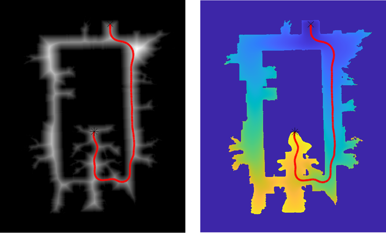
Figure 2. From left to right: velocity map, time of arrival of the wavefront
 $T(x)$
. The path obtained with FM
$T(x)$
. The path obtained with FM
 $\, ^2$
is shown as a red line.
$\, ^2$
is shown as a red line.
The FM
 $\, ^2$
method has some additional properties that make it very practical to use as a path planner [Reference Gómez, Lumbier, Garrido and Moreno23, Reference Alvarez, Lumbier, Gomez, Garrido and Moreno24]. The most important are:
$\, ^2$
method has some additional properties that make it very practical to use as a path planner [Reference Gómez, Lumbier, Garrido and Moreno23, Reference Alvarez, Lumbier, Gomez, Garrido and Moreno24]. The most important are:
-
No local minima: as long as only one wavefront is used to generate the time of arrival map, the FM
 $^2$
method ensures that there is only one global minimum in the wave source point (target point of the path).
$^2$
method ensures that there is only one global minimum in the wave source point (target point of the path). -
Completeness: the method finds a path if it exists and notifies in case of no feasible path.
-
Fast response: if the map is static, the velocity map is only calculated once. Since the FMM can be implemented with a complexity order of
$O(n)$
[Reference Yatziv, Bartesaghi and Sapiro17], building the velocity map is a fast process.


4. DE Filter
The DE method is an evolutive filter designed to solve global optimization problems over continuous spaces, proposed by Storn and Price [Reference Storn and Price25].
The evolutive filter uses a direct parallel search method that uses parameter vectors of
 $n$
dimensions
$n$
dimensions
 $x_i^k=(x_{i,1}^k,\ldots,x_{i,n}^k)^T$
to point each candidate solution
$x_i^k=(x_{i,1}^k,\ldots,x_{i,n}^k)^T$
to point each candidate solution
 $i$
to the optimization problem in each iteration step
$i$
to the optimization problem in each iteration step
 $k$
. This method uses
$k$
. This method uses
 $N$
parameter vectors
$N$
parameter vectors
 $\{ x_i^k;i=0,1,\ldots,N \}$
as a population for every generation
$\{ x_i^k;i=0,1,\ldots,N \}$
as a population for every generation
 $t$
of the optimization process.
$t$
of the optimization process.
The initial population is chosen arbitrarily to uniformly cover the whole parameter space. In the absence of a priori information, the whole parameter space has the same probability to contain the optimal parameter vector and a uniform probability distribution is assumed.
The evolutive filter generates new parameter vectors by adding the weighted difference vector between two population members to a third member, as it can be seen in Fig. 3. If the resulting vector yields a lower objective function value than the corresponding member of the previous population, the newly generated vector replaces the one which with it was compared; otherwise, the old vector is conserved.

Figure 3. Generation of a new population member.
This basic idea is extended by perturbing an existing vector through the addition of one or more weighed difference vectors. This perturbation scheme generates a variation
 $v$
according to the following equation:
$v$
according to the following equation:
 \begin{equation} v=x_i^k+L\left(x_b^k-x_i^k\right)+F\left(x_{r2}^k-x_{r3}^k\right) \end{equation}
where
 $x_i^k$
is the parameter vector to be perturbed in iteration
$x_i^k$
is the parameter vector to be perturbed in iteration
 $k$
,
$k$
,
 $x_b^k$
is the best parameter vector of the population in iteration
$x_b^k$
is the best parameter vector of the population in iteration
 $k$
and
$k$
and
 $x_{r2}^k$
y
$x_{r2}^k$
y
 $x_{r3}^k$
are the parameter vectors randomly chosen from the rest of the population.
$x_{r3}^k$
are the parameter vectors randomly chosen from the rest of the population.
 $L$
y
$L$
y
 $F$
are real and constant factors that control the amplification of the differential variables
$F$
are real and constant factors that control the amplification of the differential variables
 $(x_b^k-x_i^k)$
y
$(x_b^k-x_i^k)$
y
 $(x_{r2}^k-x_{r3}^k)$
.
$(x_{r2}^k-x_{r3}^k)$
.
The use of the best population vector in
 $x_i^k$
, which represents a mutation of the best candidate, is possible since we do not need the population to have a large diversity because the search performed is going to be local, which leads to a faster convergence. The limitation of this search to a local area is feasible due to the combination of DE with FM
$x_i^k$
, which represents a mutation of the best candidate, is possible since we do not need the population to have a large diversity because the search performed is going to be local, which leads to a faster convergence. The limitation of this search to a local area is feasible due to the combination of DE with FM
 $^2$
, as will be explained in Section 5.
$^2$
, as will be explained in Section 5.
With the purpose of incrementing the diversity of the new parameter vector generation, the crossover concept is introduced. Denoting the new parameter vector by
 $$u_i^k = {(u_{i,1}^k,u_{i,2}^k,...,u_{i,n}^k)^T}$$
with
$$u_i^k = {(u_{i,1}^k,u_{i,2}^k,...,u_{i,n}^k)^T}$$
with
 \begin{align*} u_{i,j}^k = \begin{cases} v_{i,j}^k &\quad if \; p_{i,j}^k\lt \delta \\ \\[-7pt] x_{i,j}^k &\quad if \; p_{i,j}^k \ge \delta \\ \end{cases} \end{align*}
where
 $v_{i,j}^k$
is the exchanged parameter in member
$v_{i,j}^k$
is the exchanged parameter in member
 $u_{i,j}^k$
,
$u_{i,j}^k$
,
 $p_{i,j}^k$
is a random value in the interval
$p_{i,j}^k$
is a random value in the interval
 $[0,1]$
for each parameter
$[0,1]$
for each parameter
 $j$
of the population member
$j$
of the population member
 $i$
in step
$i$
in step
 $k$
and
$k$
and
 $\delta$
is the crossover probability and constitutes the crossover control variable. Random values
$\delta$
is the crossover probability and constitutes the crossover control variable. Random values
 $p_{i,j}^k$
are created for each trial vector
$p_{i,j}^k$
are created for each trial vector
 $i$
.
$i$
.
To decide whether or not vector
 $u_i^k$
should become a member of generation
$u_i^k$
should become a member of generation
 $i+1$
, the new vector is compared to
$i+1$
, the new vector is compared to
 $x_i^k$
. If vector
$x_i^k$
. If vector
 $u_i^k$
yields a better value of the objective function than
$u_i^k$
yields a better value of the objective function than
 $x_i^k$
, then
$x_i^k$
, then
 $x_i^k$
is replaced by
$x_i^k$
is replaced by
 $u_i^{k+1}$
; on the contrary, the old value
$u_i^{k+1}$
; on the contrary, the old value
 $x_i^k$
is saved for the next generation.
$x_i^k$
is saved for the next generation.
5. Geometrically restricted path planning
The FM
 $\, ^2$
method, as explained before, can be interpreted as a vector field that repels from obstacles and is directed to the selected goal point. If the time axis is added to the wave propagation, the result is a funnel potential with one global minimum, as shown in Fig. 4. This means that the path to the goal point can be generated by the gradient descent method, keeping a safe distance from obstacles.
$\, ^2$
method, as explained before, can be interpreted as a vector field that repels from obstacles and is directed to the selected goal point. If the time axis is added to the wave propagation, the result is a funnel potential with one global minimum, as shown in Fig. 4. This means that the path to the goal point can be generated by the gradient descent method, keeping a safe distance from obstacles.
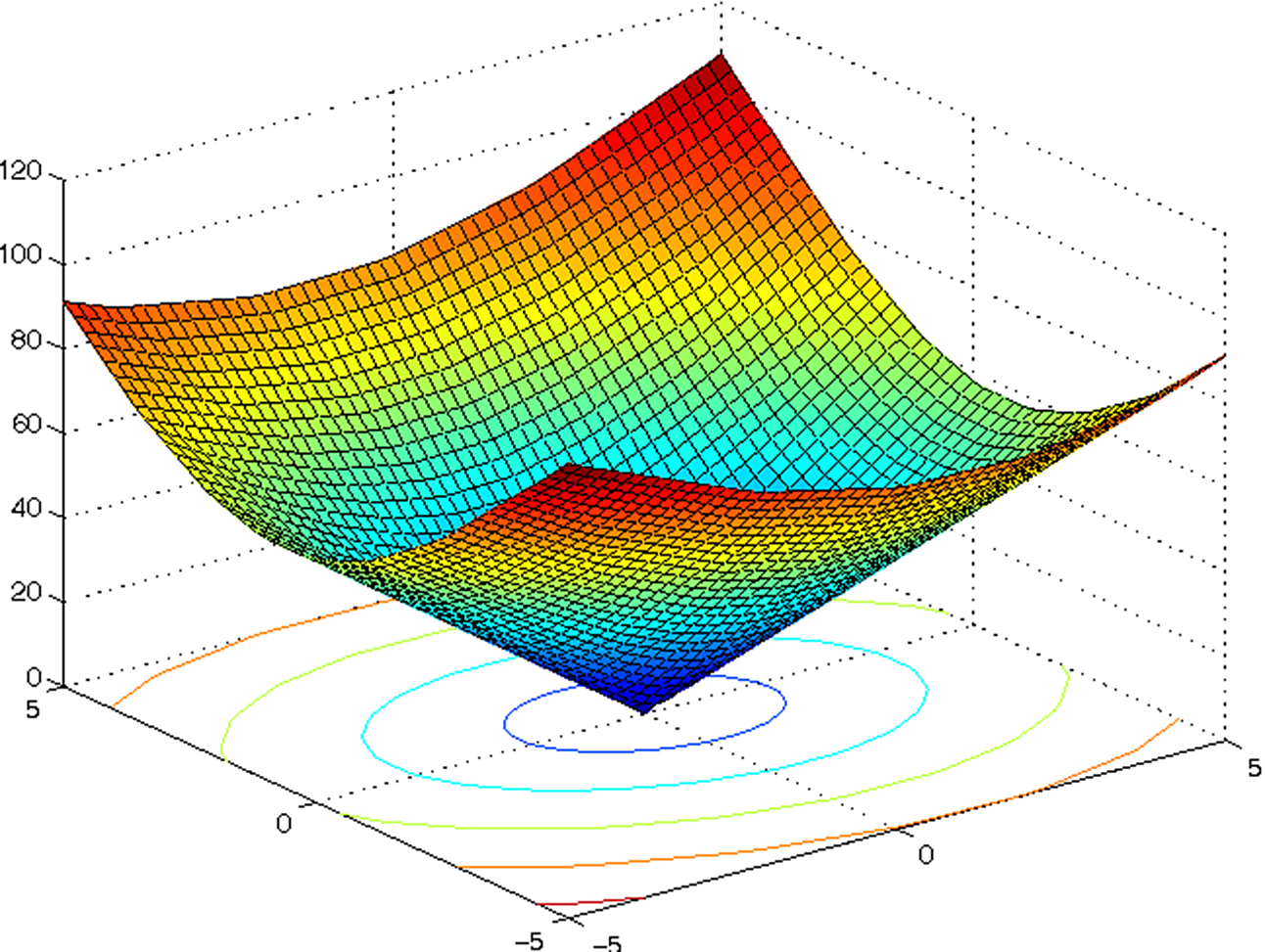
Figure 4. Funnel potential generated with FM
 $\, ^2$
.
$\, ^2$
.
The main issue with applying this method to the path planning of real robots is that it assumes a point-like system with no cinematic restrictions on its movements. If the objective is to deal with the geometric restrictions of a kinematic chain or a given task using FM
 $\, ^2$
, these restrictions need to be included in the path generation process [Reference Alvarez, Gomez, Garrido and Moreno26, Reference lvarez Sánchez27].
$\, ^2$
, these restrictions need to be included in the path generation process [Reference Alvarez, Gomez, Garrido and Moreno26, Reference lvarez Sánchez27].
5.1. Robotic hand planning
The robotic hand used in this work is the Gifu III [Reference Kawasaki, Komatsu and Uchiyama28]. The hand has five fingers, controlled by four angles:
 $\gamma$
,
$\gamma$
,
 $\beta$
,
$\beta$
,
 $\alpha$
and
$\alpha$
and
 $\theta$
. An schematic can be seen in Fig. 5.
$\theta$
. An schematic can be seen in Fig. 5.
-
$\gamma$
controls the adduction/abduction movement of all fingers.
-
$\alpha$
controls the flexion/extension movement of the first phalanx of the finger.
-
$\beta$
controls the flexion/extension movement of the second phalanx of the finger.
-
$\theta$
controls the flexion/extension movement of the third phalanx of the finger.


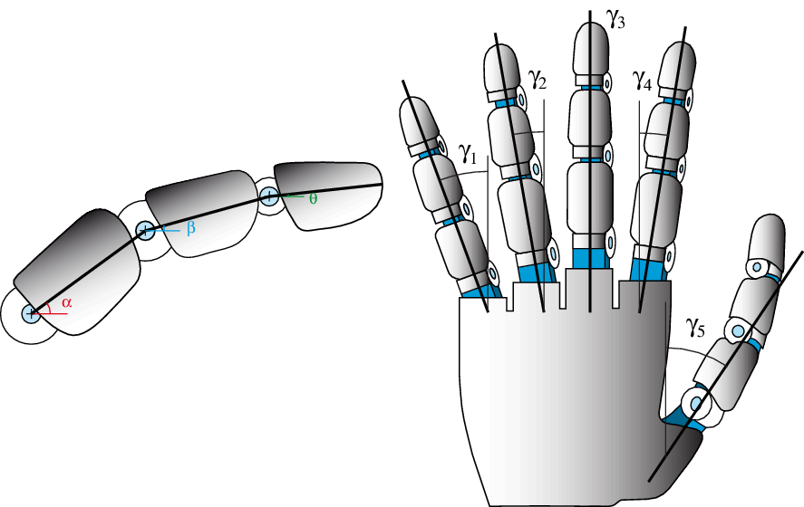
Figure 5. Angles that control the movements of the fingers of the Gifu III hand.
State-of-the-art robotic grasping methods use different techniques to obtain the final grasping configuration. Lin Shao et al. [Reference Shao, Ferreira, Jorda, Nambiar, Luo, Solowjow, Ojea, Khatib and Bohg29] propose a novel deep neural network (UniGrasp) that considers the geometry of the object to grasp and the attributes of the manipulator to obtain sets of contact points over the point cloud of the object. The proposed model is trained with a large database to produce contact points that form a force grasp and are reachable by the robotic hand. As in any neural network, inputs are introduced and outputs are generated from them. First, the features of the manipulator and the object are mapped separately in a lower dimensional space. Then, their representations are concatenated and fed as input to the neural network, which generates the contact points. This method is very practical because, unlike other methods, it is not trained for a single type of manipulator but allows manipulators to be generalized. This fact enables a robot to work with several interchangeable or upgraded manipulators without requiring training. Brahmbhatt et al. [Reference Brahmbhatt, Handa, Hays and Fox30] use a database with examples of humans grasping various household objects and synthesize functional grips for three hand models and two possible targets for those grips. The method focuses on obtaining functional grasps, which allow a task to be performed right away with the grasped object. To do this, they first sample a series of grasps on the object using the GraspIt! [Reference Miller and Allen31] simulator. From the human grasps, each point of contact is classified as attractive or repulsive. An optimization process is then performed to obtain the grips that best match the specified functionality requirements using a
 $L$
metric. Qipeng Gu et al. [Reference Gu, Su and Bi32] use a convolutional neural network (AGN: Attention Grasp Network) that uses images of objects as inputs and returns grasps for those objects. The method has been shown to take only 22ms to run and has obtained 97.8% accuracy on the Cornell grasp database. The neural network calculates a grasp for each pixel in the image, and then the set of grasps forms a grasp map. From this grasp map, the points with the highest grasp quality in the grasp map are identified as the optimal grasp.
$L$
metric. Qipeng Gu et al. [Reference Gu, Su and Bi32] use a convolutional neural network (AGN: Attention Grasp Network) that uses images of objects as inputs and returns grasps for those objects. The method has been shown to take only 22ms to run and has obtained 97.8% accuracy on the Cornell grasp database. The neural network calculates a grasp for each pixel in the image, and then the set of grasps forms a grasp map. From this grasp map, the points with the highest grasp quality in the grasp map are identified as the optimal grasp.
The goal of the path planning algorithm is to get every fingertip to its predefined grasp point on the surface of the object, minimizing unnecessary movements and taking into account the geometric restraints of the hand. Since the main focus of this work is to plan the trajectories to reach these final grasping points, grasping force analysis is not necessary, since they are not taken into account. The grasping points are selected by human imitation. The grasps performed in this work are precision grasps, so the palm of the hand is not in contact with the surface of the object.
The proposed algorithm combines planning with FM
 $\, ^2$
and optimization with an evolutive filter based on DE. The variables to control are
$\, ^2$
and optimization with an evolutive filter based on DE. The variables to control are
 $\alpha$
and
$\alpha$
and
 $\beta$
, while
$\beta$
, while
 $\gamma$
and
$\gamma$
and
 $\theta$
remain constant. This choice is made due to the fact that the complexity of the path planning process gets higher as the degrees of freedom increase, and in this case two degrees of freedom are enough to achieve satisfactory results.
$\theta$
remain constant. This choice is made due to the fact that the complexity of the path planning process gets higher as the degrees of freedom increase, and in this case two degrees of freedom are enough to achieve satisfactory results.
By applying an optimization method to solve the path planning problem, the inverse kinematics of the hand is solved iteratively. This fact makes the obtention of the optimized path a lot simpler, since calculating the inverse kinematics of a system is a complex task. The Gifu III hand has 20 degrees of freedom, while common robotic arms have six or seven. This gives an idea of the complexity of the task and the high computational cost that would be needed to calculate the inverse kinematics of this hand.
Considering both starting and target positions of each fingertip, a potential
 $D$
is calculated for every finger with FM
$D$
is calculated for every finger with FM
 $\, ^2$
. The search space used for the optimization process is formed by the joint variables
$\, ^2$
. The search space used for the optimization process is formed by the joint variables
 $\alpha$
and
$\alpha$
and
 $\beta$
. To be able to use the potential
$\beta$
. To be able to use the potential
 $D$
in the optimization process, the forward cinematics of each finger are calculated to know the position of each fingertip in the 3D cartesian space. Furthermore, it is intended that the search is conducted in a local area of the cartesian space, where the
$D$
in the optimization process, the forward cinematics of each finger are calculated to know the position of each fingertip in the 3D cartesian space. Furthermore, it is intended that the search is conducted in a local area of the cartesian space, where the
 $D$
potential is defined. This is achieved by limiting the angular expansion in each iteration of the optimization process, and penalizing every solution that is far from the initial point of that iteration with a high cost value.
$D$
potential is defined. This is achieved by limiting the angular expansion in each iteration of the optimization process, and penalizing every solution that is far from the initial point of that iteration with a high cost value.
The cost function used with the DE method to calculate the paths from the potential functions is shown in Eq. (3):
 \begin{align} \textbf{X}&=[\alpha,\beta ] \nonumber\\[3pt] i&=[x,y,z]=FK_{finger}(\gamma,\theta,\alpha,\beta ) \nonumber\\[3pt] cost &= \begin{cases} max(D) &\quad if \; d_E(i,best_{k-1}) \ge 1\\ \\[-7pt] D(i) &\quad if \; d_E(i,best_{k-1}) \lt 1\\ \end{cases} \end{align}
where
 $\textbf{X}$
is the parameter vector of the optimization process,
$\textbf{X}$
is the parameter vector of the optimization process,
 $FK_{finger}$
is the forward kinematics function of the finger,
$FK_{finger}$
is the forward kinematics function of the finger,
 $best_{k-1}$
is the last solution of the DE algorithm,
$best_{k-1}$
is the last solution of the DE algorithm,
 $d_E$
is the euclidean distance and
$d_E$
is the euclidean distance and
 $D$
is the potential function of the fingertip. In this case, the path optimization process is done five times, one for each finger.
$D$
is the potential function of the fingertip. In this case, the path optimization process is done five times, one for each finger.
To start the path calculation process, the wrist of the hand is moved to its final position and orientation, in a way that it is only necessary to move the fingers to reach the target configuration, as shown in Fig. 6.

Figure 6. Position from where the hand is closed and the path optimization process is initiated.
Figure 7 shows the path optimization process. For each finger, the initial position and the final position reached after the path generation is shown in green. The red dots indicate the evolution of the fingertip positions for every iteration of the DE algorithm. Lastly, the blue lines represent the paths calculated using the gradient descent method instead of the DE optimization process. As it can be seen, the paths obtained with the gradient descent method are less ergonomic and do not take into account the kinematic restrictions of the fingers. Furthermore, it would be necessary to calculate the inverse kinematics for each finger given the path, which as stated before, would mean a high computational cost. That is what makes methods like the one laid out in this paper necessary, in order to comply with the kinematics of the robot and avoid calculating the inverse kinematics.
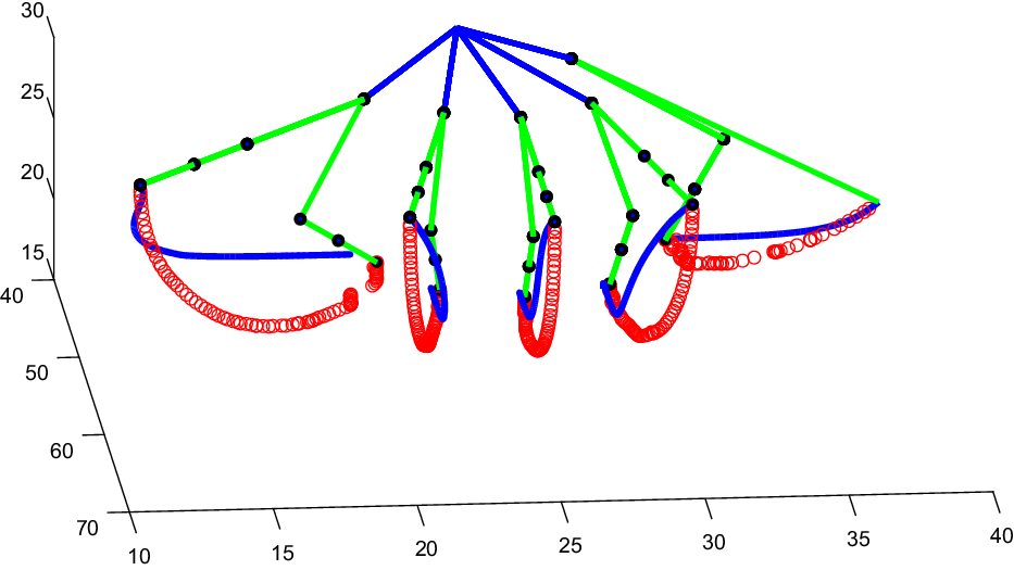
Figure 7. Paths obtained for every finger. The optimized paths obtained with DE are shown in red, while the paths obtained with the gradient descent method are shown in blue.
The result of the path generation process and the grasping of the object can be seen in Fig. 8. The figure shows that all fingertips make contact with the surface of the object and reach their final grasping position.

Figure 8. Fingertip positions after finishing the grasping process.
5.2. Robotic arm planning
Once the planning of the fingers is completed, it is necessary to plan the movements of the robotic arm, so the wrist reaches the target position and orientation and the grasping can be performed.
To start planning the movements of the robotic arm, first it is necessary to define its structure. The robotic arm used in this work is a UR3 robot from Universal Robots, as shown in Fig. 9.
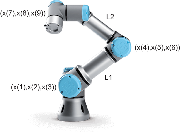
Figure 9. Scheme of the robotic arm to control, a collaborative robot UR3 from Universal Robots.
The aim of the planning is to bring the wrist point of the manipulator to the desired grasping point while avoiding obstacles, minimizing unnecessary movements and respecting the kinematic constraints of the manipulator. To achieve that, the same method used to plan the movements of the robotic hand is applied here.
In this case, the variables to control are the positions of the base, the elbow and the wrist point of the arm. The variables that make up the UR3 manipulator system are exposed below and shown in Fig. 9:
-
$x(1),x(2),x(3)$
represent the 3D coordinates of the arm’s base.
-
$x(4),x(5),x(6)$
represent the 3D coordinates of the arm’s elbow.
-
•
$x(7),x(8),x(9)$
represent the 3D coordinates of the arm’s wrist point. -
•
$L_1$
represents the length of the manipulator’s forearm. -
•
$L_2$
represents the length of the manipulator’s arm.


The cost function used with the DE method to calculate the robotic arm’s path is shown in Eq. (4):
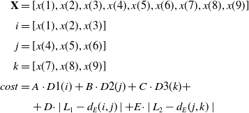 \begin{align} \textbf{X} & =[x(1),x(2),x(3),x(4),x(5),x(6),x(7),x(8),x(9)] \nonumber\\[3pt] i &=[x(1),x(2),x(3)]\nonumber\\[3pt] j &=[x(4),x(5),x(6)]\nonumber\\[3pt] k &=[x(7),x(8),x(9)]\nonumber\\[3pt] cost &= A \cdot D1(i) + B \cdot D2(j) + C \cdot D3(k) + \nonumber\\[3pt] &\quad + D \cdot \mid L_1 - d_E(i,j) \mid + E \cdot \mid L_2 - d_E(j,k) \mid \end{align}
where
 $\textbf{X}$
is the parameter vector of the optimization process,
$\textbf{X}$
is the parameter vector of the optimization process,
 $D1, D2$
and
$D1, D2$
and
 $D3$
are the potential functions of the base, elbow and wrist of the robotic arm and parameters
$D3$
are the potential functions of the base, elbow and wrist of the robotic arm and parameters
 $A,B,C,D$
and
$A,B,C,D$
and
 $E$
are constants to adjust the weights of the cost function. In this case,
$E$
are constants to adjust the weights of the cost function. In this case,
 $A=B=C=0$
.
$A=B=C=0$
.
 $2$
and
$2$
and
 $D=E=0$
.
$D=E=0$
.
 $01$
. Terms
$01$
. Terms
 $A$
,
$A$
,
 $B$
and
$B$
and
 $C$
set the weight given to the obtained trajectory trying to follow the potential function obtained with FM
$C$
set the weight given to the obtained trajectory trying to follow the potential function obtained with FM
 $\, ^2$
, while constants
$\, ^2$
, while constants
 $D$
and
$D$
and
 $E$
adjust the way in which the kinematic restrictions of the manipulator are respected, that is, the length of its arm and forearm. The values for these constants are chosen so the part of the function ensuring the length restrictions of the arm and the one that follows the potential function have a similar order of magnitude and the optimization process is fast and precise. Similar tests were ran to reach the final values used in the cost function.
$E$
adjust the way in which the kinematic restrictions of the manipulator are respected, that is, the length of its arm and forearm. The values for these constants are chosen so the part of the function ensuring the length restrictions of the arm and the one that follows the potential function have a similar order of magnitude and the optimization process is fast and precise. Similar tests were ran to reach the final values used in the cost function.
Once the objective function is implemented, some tests are ran in a closed virtual environment with the manipulator and a rectangle-shaped obstacle to study the behavior of the manipulator and the quality of the obtained path. The collision with obstacles is checked every iteration, and in case of a collision, the cost function is given a high value to discard that member of the population. Results are shown in Fig. 10.

Figure 10. Path planning for the robotic arm. The waypoints of the paths of the base, elbow and wrist are shown as red circles. The arm successfully avoids a collision with the obstacle by modifying the elbow’s path.
6. Results
Once the DE and FM
 $\, ^2$
path planning method has been designed for both the robotic arm and hand, some tests are created in a virtual environment to study its behavior in real situations.
$\, ^2$
path planning method has been designed for both the robotic arm and hand, some tests are created in a virtual environment to study its behavior in real situations.
The robot used for the simulations is the RB1 UR3 robot shown in Fig. 11. The robot consists of a mobile base with two UR3 manipulators from Universal Robots acting as arms.

Figure 11. RB1 UR3 robot used in the experiment.
First, the path for the robotic hand is planned from the desired target configuration. Due to the fact that this work focuses on the planning of the trajectories, the desired contact points are given. The pseudocode for the hand planning algorithm is shown below:

Algorithm 1. Robotic hand planning.
Once the paths for the robotic hand are computed, it is turn for the robotic arm. This algorithm takes the desired target position of the wrist and a map of the environment and calculates a collision-free path.

Algorithm 2. Robotic arm planning.
In conventional industrial applications, the planning is only done for the wrist point of the robot. In this case, however, it is imperative to plan for the wrist as well as the shoulder and elbow, as the planning tasks to be performed involve scenarios with many obstacles and objects to avoid.
Once the movements of the manipulator and the hand have been planned, the hand and manipulator are moved in a coordinated way from the initial to the final configuration. This is achieved using a leader–follower approach, where the wrist point is the leader and the hand joints are the followers.

Algorithm 3. Coordinated hand-arm movement.
For every waypoint of the wrist point’s path, the joint values stored during the path planning process are used to calculate the 3D positions of the followers using forward kinematics. The hand’s orientation in each point is calculated with the function trinterp from Peter Corke’s Robotic Toolbox [Reference Corke33], from the starting and ending homogeneous transformation matrices.
Once the algorithms designed in this work have been explained, we proceed to explain the decisions that have led to the design of an experiment to test their effectiveness and possible applications. Since the R1 UR3 robot will be used to assist people, it is necessary to test how it performs in environments normally occupied by humans. A good test that suits these characteristics is to grasp objects with different shapes and orientations placed on a table. In this case, it is assumed that the base of the RB1 UR3 robot remains stationary, so the shoulder position is fixed and only the elbow and wrist trajectories are planned.
The tests for both algorithms are performed in Matlab with a simulated version of the RB1 UR3 robot since the real robot is available but does not have a robotic hand for testing. The algorithm that plans the paths for the robotic arm has been tested on the real robot. The simulations performed are enough to detect in advance major issues in the future behavior of the robot coming from our planning algorithms, since the variables used for the path planning testing are the position of the base of the UR3 manipulator and its link lengths, and the palm size and finger lengths for the Gifu III hand. The scenario in which the simulations are going to be performed is shown in Fig. 12. The stage has the robotic arm with the shoulder placed in the position that would correspond to the R1 UR3 robot and a table located at a height of 87 cm on which the objects to be grasped are placed.
The algorithm parameters used in each phase are shown in Table I.
Table I. Simulation parameters.


Figure 12. Environment used for the simulations. The stage consists of a UR3 manipulator and a table located at a height of 87 cm.
Grasping tests are performed with a cube, a cylinder, a sphere, a rotated cube and a lying cylinder. The tests consist of the grasping of every object 1000 times. The reason for selecting these objects is that most everyday objects can approximate one of these primitive shapes. The number 1000 has been selected to test the stochastic nature of the DE algorithm. The figures of the grasping process obtained can be seen in subsection 7. Table II shows the mean and standard deviation of the execution times obtained for the algorithm with every object. The tests were ran on a Mountain Onyx laptop with 16 GB of RAM and an Intel(R) Core(TM) i7-4720HQ CPU 2.60 GHz processor.
Table II. Execution times obtained from the simulations.
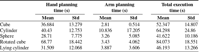
Due to the stochastic nature of the algorithm, the standard deviation is high on average. The fact that the planning algorithm stops when the fingertip or arm joint reaches a position within 0.5 cm of their target position also affects the standard deviation. The success rate of this experiments is 100 %, given the high number of maximum iterations and members of the population.
In view of the results obtained, it can be safely stated that the Fast Marching and DE path planning algorithm can be extrapolated to all types of objects and scenes.
6.1. Experimental results
To further prove the functionality of the algorithm, an experiment is performed on the real robot. Since we do not have a robotic hand available yet, the algorithm tested is the one that controls the movement of the robotic arm. The robotic platform used can be seen in Fig. 13.
In this experiment, a target position is given to the left arm of the robot. The path for the arm is then computed using the proposed algorithm. The resulting path can be seen in Fig. 14. For a recorded demonstration of the experiment see this video.

Figure 13. Real RB1 UR3 robot used in the experiment.

Figure 14. Path calculated with the proposed algorithm.
This experiment shows that the implementation of the algorithm in simulations can be easily moved to the real robot, since the robot model and the parameters used are the same. The algorithm that plans the paths for the robotic hand will be tested in a future version of the paper when one is available.
7. Conclusion
The main objective of this work has been to study and implement a geometrically constrained path planning method for robotic grasping with DE and FM2. The algorithm has been implemented in Matlab to test its performance in different simulated scenarios and on the real robot.
The combination of the FMM with the DE evolutionary filter makes it possible to solve all kinds of problems related to path planning. The FMM allows to generate a funnel function that plans trajectories that guide the hand-manipulator set toward its goal and the DE evolutionary filter allows to use a cost function that is in charge of calculating an optimized trajectory that meets the kinematic constraints of the joints of the set and avoids collisions with obstacles.
In the case of the fingers of the hand, these constraints are those shaped by the rigid links of the hand, while in the case of the manipulator these constraints are determined by the rigid links of the manipulator. In addition, a leader–follower formation approach is used to control the positions of the finger joints from the wrist point along the path.
Finally, simulations and an experiment with the real robot are performed with the RB1 UR3 robot in an environment with a table on which different objects are placed to test the performance of the algorithm and its versatility.
In conclusion, an algorithm capable of planning trajectories for the desired manipulation tasks and implementable in a real robot such as the RB1 UR3 has been developed, thus fulfilling the objectives established for this work.
Conflicts of interest
The authors declare no conflicts of interest.
Financial support
This work was supported by the funding from HEROITEA: Heterogeneous Intelligent Multi-Robot Team for Assistance of Elderly People (RTI2018-095599-B-C21), funded by Spanish Ministerio de Economía y Competitividad.
Ethical considerations
None
Author’s contributions
Conceptualization, Javier Muñoz.; methodology design, Santiago Garrido and Luis Moreno; software, Javier Muñoz; validation, Blanca López; formal analysis, Fernando Quevedo; and project administration, Ramón Barber. All authors have read and agreed to the published version of the manuscript.
A. Appendix A
On the left, the initial configuration of the test. On the right, the final configuration reached after applying the path planning algorithm.

Figure 15. Results for the cube grasping test.

Figure 16. Results for the cylinder grasping test.

Figure 17. Results for the sphere grasping test.

Figure 18. Results for the rotated cube grasping test.

Figure 19. Results for the lying cylinder grasping test.


 Open access