


1. Introduction
The phenomenon of a droplet impacted by shock waves occurs widely in natural and industrial scenarios such as two-phase supersonic combustors (Malik et al. Reference Malik, Hytovick, Chin, Burke, Rezzag, Stiehl, Morales and Ahmed2022), supernova explosions (Abgrall & Karni Reference Abgrall and Karni2001), cavitation (Brennen Reference Brennen2013) and shock wave lithotripsy (Johnsen & Colonius Reference Johnsen and Colonius2009). In the development of hypersonic propulsion systems, in particular, it is of great interest to understand the behaviours of fuel droplets interacting with shock waves. In previous studies, this thread of investigations has mainly been presented in regard to three aspects, which are: the deformation mechanism of the shocked droplet, the wave evolution characteristics and the cavitation behaviours inside the shocked droplet.
Over the past decades, continuous efforts to reveal the deformation and breakup mechanism of the shocked droplet or liquid column have been made via theoretical analyses, experimental investigations and numerical simulations. As a classical result, the breakup modes of droplets, without the impacts of the shock wave, are classified into five regimes denoted as vibrational, bag, bag and stamen, stripping and catastrophic breakup, which are described in the works of Pilch & Erdman (Reference Pilch and Erdman1987) and Hsiang & Faeth (Reference Hsiang and Faeth1992, Reference Hsiang and Faeth1993). Furthermore, Theofanous, Li & Dinh (Reference Theofanous, Li and Dinh2004) and Theofanous & Li (Reference Theofanous and Li2008) reclassified the breakup modes into two regimes with consideration of the effect of incident shock wave impaction, namely the Rayleigh–Taylor piercing mode and shear-induced entrainment mode. Meng & Colonius (Reference Meng and Colonius2015) numerically studied the interaction of a planar shock wave with a water column and described the deformation characteristics of the water column under different shock wave intensities. Then, Meng & Colonius (Reference Meng and Colonius2018) studied the interaction between a planar shock and a spherical droplet, hence analysing the droplet deformation characteristics. Through high-magnification and high-speed breakup images, Biasiori-Poulanges & El-Rabii (Reference Biasiori-Poulanges and El-Rabii2019) demonstrated the evolution dynamics of the breakup process at a higher Weber number. Sharma et al. (Reference Sharma, Pratap Singh, Srinivas Rao, Kumar and Basu2021) detailly investigated the initial wave dynamics and droplet breakup dynamics of the interaction dynamics between a liquid droplet and a planar shock wave in a wide range of Weber numbers and Reynolds numbers.
In this area of study, the evolution characteristics of waves inside a droplet are still a subject that is under studied. Igra & Takayama (Reference Igra and Takayama2001a,Reference Igra and Takayamab), Igra & Sun (Reference Igra and Sun2010) and Meng & Colonius (Reference Meng and Colonius2015) showed that early stages of shock wave propagation events inside the liquid droplet are an inherent part of the aero-breakup problem. In addition, Igra & Sun (Reference Igra and Sun2010) pointed out that the two-dimensional cylindrical water column behaves similarly to a spherical droplet when comparing droplet deformation and disintegration. However, considering the transient time scale, visualising the complex wave structures propagating inside the spherical droplet presents a huge challenge in experimental studies. Numerous studies have been the primary choice in investigating the flow characteristics inside a liquid column. Sembian et al. (Reference Sembian, Liverts, Tillmark and Apazidis2016) detailly reported the wave structure evolution at the early stages of planar shock wave interaction with a cylindrical water column under different incident shock wave intensities. The work revealed the evolution characteristics of the wave structures inside the liquid column impinged by a planar shock wave. Boyd & Jarrahbashi (Reference Boyd and Jarrahbashi2021) extended the shock–droplet interaction problem from the subcritical condition to the supercritical condition and studied the effects of temperature, pressure and shock intensity on the interaction. Based on the ray analysis method (Heymann Reference Heymann1969; Haller et al. Reference Haller, Poulikakos, Ventikos and Monkewitz2003; Wu, Xiang & Wang Reference Wu, Xiang and Wang2018), Biasiori-Poulanges & El-Rabii (Reference Biasiori-Poulanges and El-Rabii2021) theoretically investigated the interaction of a planar shock wave with a liquid column and derived the concentration of rays with different reflection times and then verified their results by numerical simulations. Guan et al. (Reference Guan, Liu, Wen and Shen2018) numerically and theoretically investigated the establishment of an internal flow field inside a water droplet subjected to shock wave impact. In their work, a saddle point inside the water droplet is observed for the first time, chosen as a characteristic point to describe the internal flow.
In the current literature, it has been stated that the propagating expansion waves inside the droplet can induce a cavitation phenomenon. However, the criteria are yet to be established since the process is highly transient. The possibility of cavitation in the water column due to the expansion wave focusing at higher shock Mach numbers was observed in the works of Sembian et al. (Reference Sembian, Liverts, Tillmark and Apazidis2016). Field, Dear & Ogren (Reference Field, Dear and Ogren1989) and Field et al. (Reference Field, Camus, Tinguely, Obreschkow and Farhat2012) observed that, when a high-speed droplet impacts a rigid wall, convergence of reflected expansion waves could cause cavitation bubbles. The possibility of cavitation of a high-speed droplet impacting the wall was verified by Kondo & Ando (Reference Kondo and Ando2016), Wu et al. (Reference Wu, Xiang and Wang2018) and Wu, Liu & Wang (Reference Wu, Liu and Wang2021b) via the numerical method. Xiang & Wang (Reference Xiang and Wang2017) and Biasiori-Poulanges & El-Rabii (Reference Biasiori-Poulanges and El-Rabii2021) expounded that the occurrence of cavitation inside the shocked water column is dependent on the incident shock wave intensity and the value of the cavitation threshold pressure. Moreover, Xiang & Wang (Reference Xiang and Wang2017) performed a numerical study on the interaction of a planar shock wave with a water column embedded with air cavities of different sizes at high Weber numbers. Liang et al. (Reference Liang, Jiang, Wen and Liu2020) captured the deformation of a water droplet embedded within a vapour cavity and analysed the influence of the relative size and eccentricity of the vapour cavity on the mechanism of droplet deformation. The results show that the embedded cavity inside the water column or droplet can significantly affect the deformation characteristics.
Summarising the past decades, the planar shock wave interacting with a liquid droplet/column has been widely studied, and the droplet deformation and the inherent evolution characteristics of wave structures have been well investigated experimentally, numerically and theoretically. However, in some practical application scenarios, such as the ultrasound-assisted treatment of human tissues (Feril & Kondo Reference Feril and Kondo2004; Kim et al. Reference Kim, Rhim, Choi, Lim and Choi2008; Lukka et al. Reference Lukka, Waldron, Chin, Mayhew, Warde, Winquist, Rodrigues and Shayegan2010), it is quite hard for the wavefront to achieve an ideal plane (Sembian et al. Reference Sembian, Liverts, Tillmark and Apazidis2016). Moreover, Mittelstein et al. (Reference Mittelstein, Ye, Schibber, Roychoudhury, Martinez, Fekrazad, Ortiz, Lee, Shapiro and Gharib2020) and Landgraf et al. (Reference Landgraf, Kozlowski, Zhang, Fournelle, Becker, Tretbar and Melzer2022) reported that, in obtaining the desirable cavitation phenomena, e.g. the micro-bubble cavitation process as being an enhancer of bioeffects reported by Feril & Kondo (Reference Feril and Kondo2004), the regulation of the location of the focus point and the negative pressure intensity near the focus point are critical. For this reason, the utilisation of the cavitation effect is subject to a certain deviation when only the influence of the planar shock wave intensity is considered. In addition, even when an ideal planar shock wave would be achieved by more advanced technologies, simultaneously achieving precise regulation of the focus point position and the negative-pressure intensity by adjusting the intensity of the incident wave remains a challenge. In this context, it is of interest to reveal the effects of the incident shock wave shape on the focus point location and negative pressure intensity. Therefore, through theoretical analysis and numerical simulations, this study aims to investigate the wave converging phenomena inside a two-dimensional water column impinged by a curved shock wave. The findings concluded in this study are expected to help researchers attain the migration of the focus point and amplify or reduce the negative-pressure intensity near the focus point through suitable wavefront shape designs and the adjustment of the incident shock wave intensity.
This paper is organised as follows. In § 2, the physical model of the interaction between the curved shock wave and a water column is described, and the theoretical tool of the ray analysis method is established, and the governing equations, numerical treatments and numerical validation are presented. In § 3, the morphology and dynamical evolutions of wave structures are analysed qualitatively and quantitatively, taking the interaction of a cylindrical converged shock wave with a water column as an example. In § 4, the effects of intensities and shapes of the incident shock wave are investigated. Finally, the conclusions are presented in § 5.
2. Physical model and numerical procedure
2.1. Physical model
The previous study (Igra & Sun Reference Igra and Sun2010) has shown that the flow characteristics inside the two-dimensional water column are similar to those inside the spherical droplet, and that three-dimensional numerical simulation comes at a huge CPU time cost. Hence, the two-dimensional water column is chosen in the present study to save computing resources as much as possible and improve computing efficiency. A schematic diagram of the interaction of a cylindrical incident shock wave with a water column is shown in figure 1, including a converged and diverged one. We use  $R_0$ to represent the radius of the cylindrical shock wave when it just touches the water column and
  $R_D$ to represent the radius of the water column. Moreover, the dimensionless radius
  ${\omega (=R_0/R_D)}$ is used to normalise the curvature effect of the incident shock wave. Referring to the experiment (Igra & Takayama Reference Igra and Takayama2001a) and numerical simulation (Xiang & Wang Reference Xiang and Wang2017), the initial value of
  $R_D$ is taken as 2.4 mm. Moreover, we use
  $C$ and
  $O$ to represent the water column centre and the origin of coordinates, respectively. The water column and the air ahead of the shock wave are initially in equilibrium with a temperature of 300 K and a pressure of 101 325 Pa. The Weber numbers in the present numerical simulations are higher than 1000, and the corresponding Reynolds numbers are over 40 000. Therefore, the viscosity and the surface tension can be neglected in the present study (Meng & Colonius Reference Meng and Colonius2015).

Figure 1. Schematic diagram of the interaction of a cylindrical shock with a water column. (a) The interaction of a converged shock with a water column; (b) the interaction of a diverged shock with a water column.
In the present study, the generation of the cylindrical shock wave is based on the theory of shock dynamics, which can characterise the propagation of shock waves with an arbitrary profile. The Chester–Chisnell–Whitham (CCW) relation is the basis of shock dynamics for a uniform quiescent gas ahead of shock, which is referred from Chester (Reference Chester1954), Chisnell (Reference Chisnell1957) and Whitham (Reference Whitham1957, Reference Whitham1958, Reference Whitham1959). The CCW relation describes how the shock wave Mach number  $M$ varies with the shock-front area
  $A$ (
$A$ ( $= 2{\rm \pi} R$ in two-dimensional cases), which can be written as
 \begin{equation} \frac{2M\,\mathrm{d}M}{({{M}^{2}}-1)K( M )}+\frac{\mathrm{d}A}{A}=0, \end{equation}
where
 \begin{align} K( M )=2{{\left[ 2\mu +1+\frac{1}{{{M}^{2}}} \right]}^{{-}1}}{{\left[ 1+\frac{2}{\gamma +1}\left( \frac{1}{\mu }-\mu \right) \right]}^{{-}1}} ,\quad \mu =\sqrt{\frac{( \gamma -1 ){{M}^{2}}+2}{2\gamma {{M}^{2}}-( \gamma -1 )}}. \end{align}
 Zhai et al. (Reference Zhai, Liu, Qin, Yang and Luo2010) used this shock dynamics theory to design a curved wall profile (V-shaped geometry) and realised the transformation from a planar shock wave to a cylindrical converged shock wave, as shown in figure 2. Both numerical and experimental results show a perfect circular shock front. However, this method comes at enormous computing resource cost due to the large computation domain and usually can only obtain a cylindrical shock wave with a small converging angle ( $= 2\theta _0$), which leads to a small range of radius of the water column that can be investigated in the present study. Hence, a
  $90^{\circ }$ computational domain is used in this paper, as shown in figure 1(
 $a$), which is widely used in the literature (Lombardini, Pullin & Meiron Reference Lombardini, Pullin and Meiron2014; Zhai et al. Reference Zhai, Zhang, Zhou, Ding and Wen2019; Wu, Liu & Xiao Reference Wu, Liu and Xiao2021a). The fluid variables behind the cylindrical shock wave are calculated by the following algorithm: given the cylindrical shock radius of
  $R_0$, the cylindrical shock wave intensity
  $M_0$ and fluid variables ahead of the incident cylindrical shock wave
  $p_0$ and
  $T_0$. When the radius of the cylindrical shock wave is
  $R$, the intensity of the cylindrical shock wave
  $M$ satisfies
 \begin{equation}
\int_{{{M}_{0}}}^{M}{\frac{2m\,\mathrm{d}m}{({{m}^{2}}-1)K( m )}}={-}\int_{{{R}_{0}}}^{R}{\frac{\mathrm{d}r}{r}}.
\end{equation}
\begin{equation}
\int_{{{M}_{0}}}^{M}{\frac{2m\,\mathrm{d}m}{({{m}^{2}}-1)K( m )}}={-}\int_{{{R}_{0}}}^{R}{\frac{\mathrm{d}r}{r}}.
\end{equation}

Figure 2. The schematic drawing of the wall profile, transforming the planar shock into a cylindrical one. Here,  $H$ is the half-height of the V-shaped geometry;
  $l$ the length of the V-shaped geometry;
  $Ma_0$ the Mach number of the incident planar shock waves;
  $Ma_D$ the Mach number of the cylindrical shock wave;
  $\theta _0$ the half-converging angle.
Integrating (2.3) by numerical iteration, the value of  $M$ is obtained. Further, using the Rankine–Hugoniot conditions, the fluid variables behind the cylindrical shock wave can be calculated, including pressure
  $p$, density
  $\rho$, temperature
  $T$ and velocity magnitude
  $V_m$. The accuracy verification of CCW theory is presented in detail in Appendix A.
2.2. Method of the ray analysis
In this sub-section, the ray analysis method (Heymann Reference Heymann1969; Haller et al. Reference Haller, Poulikakos, Ventikos and Monkewitz2003; Wu et al. Reference Wu, Xiang and Wang2018), which is based on the Huygens principle used in the theoretical analysis of wave configurations, is presented. For convenience, two moving point disturbances, which are denoted as  $S_1$ and
  $S_2$, and a straight material interface are used to briefly introduce the ray analysis method, as shown in figure 3. At the initial instant, two moving point disturbances coincide at point
  $S_0$, located on the straight interface. Then these two point disturbances move away from
  $S_0$ in opposite directions with the same speed, which gradually decreases with distance s from
  $S_1$ (
 $S_2$) to
  $S_0$ and is denoted as
  $V(s)$. Based on the Huygens principle, an individual wavelet will be emitted at each instant at
  $S_1(s)$ and these individual wavelets propagate at a constant speed of
  $W$. It can be seen that the envelope of all individual wavelets generated before
  $t$ forms the wavefront induced by these two moving point disturbances. According to the relationship between
  $V(s)$ and
  $W$, there are four envelope shapes, as shown in figure 3(a–d). Note that, for the case corresponding to figure 3(b), when the propagation speed of the point disturbance
  $V(s)$ is less than
  $W$, the newer individual wavelets cannot catch up with the envelope of wavelets, as will be explained in detail in § 3.1.

Figure 3. Schematic diagram of the Huygens principle.
For three cases except for the case corresponding to figure 3(b), it is not difficult to understand the position and shape of the envelope of wavelets, while it is still confusing to understand the evolution characteristics of the envelope for the rest of the cases. Hence, the ray analysis method is used, as shown in figure 4. The propagation of each wavelet can be equivalent to the propagation of infinite rays emitted at its origin, and the length of the ray is equal to the propagation distance of the wavelet. It is obviously found that not all of the rays emitted from the same wavelet can effectively contribute to the envelope of wavelets. Therefore, to reveal the physical mechanism of the motion of the wavefront induced by point disturbances, it is necessary to find these special rays which have contributed to the envelope of wavelets. Here, the two wavelets emitted from  $S_s$ and
  $S_{s+\Delta s}$ are selected for detailed discussion, as shown in figure 4(b), and these two emission points are very close to each other. The radii of these two wavelets are
  $r(t,s)$ and
  $r(t, s+\Delta s)$, respectively,
 \begin{equation} r( {t,s} ) = W( {t - {t_s}} ) ,\quad {r( {t,s + \Delta s} ) = W( {t - {t_{s + \Delta s}}} )}, \end{equation}
where  $t_s$ represents the time for moving point disturbance
  $S_1$ from
  $S_0$ to
  $S_1(s)$.

Figure 4. Schematic diagram of the ray analysis method.
The intersection point of these two wavelets is  $G_s$, and the angle between the vector
  $\overrightarrow {{S_s}{S_{s+\Delta s}}}$ and
  $\overrightarrow {{S_s}{G_{s}}}$ is
  $\alpha _s$, as shown in figure 4(b). The expression
  $\alpha _s$ is derived from the law of cosines in the triangle
  $\Delta {S_s}{S_{s+\Delta s}}{G_s}$
 \begin{equation} \cos {\alpha_s} =
\frac{{( {2t - {t_s} - {t_{s + \Delta s}}} )}}{{2( {t -
{t_s}} )}} \frac{{( {{t_{s + \Delta s}} - {t_s}}
)W}}{{\Delta s}} + \frac{{\Delta s}}{{2( {t - {t_s}} )W}}.
\end{equation}
\begin{equation} \cos {\alpha_s} =
\frac{{( {2t - {t_s} - {t_{s + \Delta s}}} )}}{{2( {t -
{t_s}} )}} \frac{{( {{t_{s + \Delta s}} - {t_s}}
)W}}{{\Delta s}} + \frac{{\Delta s}}{{2( {t - {t_s}} )W}}.
\end{equation}
When  $S_{s+\Delta s}$ is infinitely close to
  $S_s$ (
 $\Delta s\to {0^+}$),
  $\alpha _s$ is the angle between the vector of the emitted ray and the material interface. The endpoint of this ray is the unique contribution of the wavelet emitted from
  $S_s$ to the envelope of wavelets
 \begin{align} \cos {\alpha_s}&=\lim_{\Delta s \to {0^ + }} \left[ {\frac{{( {2t - {t_s} - {t_{s + \Delta s}}} )}}{{2( {t - {t_s}} )}}\frac{{( {{t_{s + \Delta s}} - {t_s}} )W}}{{\Delta s}} + \frac{{\Delta s}}{{2( {t - {t_s}} )W}}} \right] \nonumber\\ &= \lim_{\Delta s \to {0^ + }} \frac{{( {{t_{s + \Delta s}} - {t_s}} )W}}{{\Delta s}} = W{t'_s}. \end{align}
Equation (2.6) shows that the emission angle of these particular rays is only determined by the propagation speed of the wavelets and the kinematic characteristics of the moving point disturbance along the material interface. Note that, if the material interface were a closed curve, these rays would reflect on the material interface after a period of propagation. This reflection property will be investigated in detail in § 3.1.
2.3. Numerical models
The interaction between the shock wave and the droplet is a strong compressible multiphase hydrodynamics problem, which involves complex factors such as a large density ratio and strong shock waves. In this paper, the numerical simulation is carried out by the in-house software (SCP-tran![]() ), which was previously applied to study a variety of compressible multiphase flow problems (Xiang & Wang Reference Xiang and Wang2017; Wang, Xiang & Hu Reference Wang, Xiang and Hu2018; Wu et al. Reference Wu, Xiang and Wang2018). The five-equation model (Allaire, Clerc & Samuel Reference Allaire, Clerc and Samuel2002; Johnsen & Colonius Reference Johnsen and Colonius2006) is used to solve the gas–liquid hydrodynamic system, and the governing equations consist of two continuity equations for each phase, a mixture momentum equation, a mixture energy equation and a volume fraction advection equation of the liquid phase
), which was previously applied to study a variety of compressible multiphase flow problems (Xiang & Wang Reference Xiang and Wang2017; Wang, Xiang & Hu Reference Wang, Xiang and Hu2018; Wu et al. Reference Wu, Xiang and Wang2018). The five-equation model (Allaire, Clerc & Samuel Reference Allaire, Clerc and Samuel2002; Johnsen & Colonius Reference Johnsen and Colonius2006) is used to solve the gas–liquid hydrodynamic system, and the governing equations consist of two continuity equations for each phase, a mixture momentum equation, a mixture energy equation and a volume fraction advection equation of the liquid phase
 \begin{equation} \left.\begin{gathered} \frac{{\partial ( {{\alpha_l}{\rho_l}} )}}{{\partial t}} + \frac{{\partial ( {{\alpha_l}{\rho_l}u} )}}{{\partial x}} + \frac{{\partial ( {{\alpha _l}{\rho_l}v} )}}{{\partial y}} = 0,\\ \frac{{\partial ( {{\alpha_g}{\rho_g}} )}}{{\partial t}} + \frac{{\partial ( {{\alpha_g}{\rho_g}u} )}}{{\partial x}} + \frac{{\partial ( {{\alpha _g}{\rho_g}v})}}{{\partial y}} = 0,\\ \frac{{\partial ( {\rho u} )}}{{\partial t}} + \frac{{\partial ( {\rho {u^2} + p} )}}{{\partial x}} + \frac{{\partial ( {\rho uv} )}}{{\partial y}} = 0,\\ \frac{{\partial ( {\rho v} )}}{{\partial t}} + \frac{{\partial ( {\rho uv} )}}{{\partial x}} + \frac{{\partial ( {\rho {v^2} + p})}}{{\partial y}} = 0,\\ \frac{{\partial \rho E}}{{\partial t}} + \frac{{\partial [ {( {\rho E + p} )u} ]}}{{\partial x}} + \frac{{\partial [ {( {\rho E + p})v} ]}}{{\partial y}} = 0,\\ \frac{{\partial {\alpha_l}}}{{\partial t}} + u\frac{{\partial {\alpha_l}}}{{\partial x}} + v\frac{{\partial {\alpha_l}}}{{\partial y}} = 0, \end{gathered}\right\} \end{equation}
where  $\rho _l$ and
  $\rho _g$ represent the density of the liquid and gas phases, respectively,
  $\alpha _l$ and
  $\alpha _g$ represent the volume fraction of the liquid and gas phases, respectively,
  $\rho$,
  $u$,
$u$,  $v$,
$v$,  $p$ and
  $E$ represent the mixture density,
  $x$-velocity,
  $y$-velocity, pressure and specific total energy, respectively. The numerical diffusion appears significant at the two-phase interface after several time steps. In this diffuse region, the mixture variables are given as (Saurel, Petitpas & Abgrall Reference Saurel, Petitpas and Abgrall2008)
 $$\begin{gather} \rho = {\alpha_l}{\rho_l} + {\alpha_g}{\rho_g}, \end{gather}$$
 $$\begin{gather}\rho E = {\alpha_l}{\rho_l}{e_l} + {\alpha_g}{\rho _g}{e_g} + \tfrac{1}{2}\rho ( {{u^2} + {v^2}} ), \end{gather}$$
 $$\begin{gather}\rho {c^2} = {\alpha_l}{\rho_l}c_l^2 + {\alpha_g}{\rho _g}c_g^2, \end{gather}$$
where  $e_l$ and
  $e_g$ represent the specific internal energy of the liquid and gas phases, respectively,
  $c_l$ and
  $c_g$ represent the sound speed of the liquid and gas phases, respectively. In this study, the stiffened gas equation of state is used to close the governing equations
 $$\begin{gather} {{\rho_k}{e_k} = \frac{{p + {\gamma_k}{p_{\infty ,k}}}}{{{\gamma_k} - 1}}} ,\quad {k = l,g}, \end{gather}$$
 $$\begin{gather}{{c_k} = \sqrt {\frac{{\left( {p + {p_{\infty ,k}}} \right){\gamma_k}}}{{{\rho_k}}}} },\quad {k = l,g}, \end{gather}$$
where  $\gamma$ is the specific heat ratio and
  $p_\infty$ is the reference pressure. For air,
  $\gamma = 1.4$ and
  $p_\infty = 0$, and the stiffened gas equation of state reduces to the ideal gas equation. Referring to the works of Kondo & Ando (Reference Kondo and Ando2016) and Xiang & Wang (Reference Xiang and Wang2017), the parameters for water are taken to be
  $\gamma = 6.12$ and
  $p_\infty = 343.44$ MPa.
2.4. Numerical treatments
The SCP-tran![]() fluid dynamic software uses a finite volume method (Titarev & Toro Reference Titarev and Toro2004) to discretise the above governing equations in a uniform Cartesian grid system. The component-wise fifth-order incremental weighted essentially non-oscillatory reconstruction is applied, as previously proposed by the present author (Wang et al. Reference Wang, Xiang and Hu2018). The Harten–Lax–van Leer contact approximate Riemann solver (Toro Reference Toro2009) is employed to solve the numerical flux at the cell face. The third-order total variation diminishing Runge–Kutta method (Gottlieb & Shu Reference Gottlieb and Shu1998) is chosen to advance the solutions over time. Considering that part of the boundaries does not coincide with the interface of the grid cell, such as the immersed non-reflecting boundary as shown in figure 1, a ghost-cell immersed boundary method (IBM) for distinguishing geometrically complex boundaries is used to realise the non-reflecting boundary condition (Thompson Reference Thompson1987, Reference Thompson1990), and for the detail of IBM the reader is referred to the works of Choung et al. (Reference Choung, Saravanan, Lee and Cho2021) and Saravanan, Choung & Lee (Reference Saravanan, Choung and Lee2021). Since the evolution characteristics of the interaction between shock waves and the water column are symmetric, to improve the calculation efficiency, the symmetric boundary condition at the axis of the liquid column is adapted to carry out numerical simulations. The numerical verification of the grid sensitivity is presented in Appendix B.
fluid dynamic software uses a finite volume method (Titarev & Toro Reference Titarev and Toro2004) to discretise the above governing equations in a uniform Cartesian grid system. The component-wise fifth-order incremental weighted essentially non-oscillatory reconstruction is applied, as previously proposed by the present author (Wang et al. Reference Wang, Xiang and Hu2018). The Harten–Lax–van Leer contact approximate Riemann solver (Toro Reference Toro2009) is employed to solve the numerical flux at the cell face. The third-order total variation diminishing Runge–Kutta method (Gottlieb & Shu Reference Gottlieb and Shu1998) is chosen to advance the solutions over time. Considering that part of the boundaries does not coincide with the interface of the grid cell, such as the immersed non-reflecting boundary as shown in figure 1, a ghost-cell immersed boundary method (IBM) for distinguishing geometrically complex boundaries is used to realise the non-reflecting boundary condition (Thompson Reference Thompson1987, Reference Thompson1990), and for the detail of IBM the reader is referred to the works of Choung et al. (Reference Choung, Saravanan, Lee and Cho2021) and Saravanan, Choung & Lee (Reference Saravanan, Choung and Lee2021). Since the evolution characteristics of the interaction between shock waves and the water column are symmetric, to improve the calculation efficiency, the symmetric boundary condition at the axis of the liquid column is adapted to carry out numerical simulations. The numerical verification of the grid sensitivity is presented in Appendix B.
2.5. Validation of the solver
Thanks to the experiments in the literature, the interaction of a planar shock wave with a water column is chosen as a validation case to validate the SCP-tran![]() fluid dynamic software. For a qualitative comparison, the dimensionless time
fluid dynamic software. For a qualitative comparison, the dimensionless time  $t^*$ is used, which is the ratio of the physical time over the characteristic time
  $\tau$ (
 $\tau = 2R_D/ V_{ts}$,
  $V_{ts}$ is the propagation speed of the transmitted shock wave). For convenience, the zero instant is marked as
  $t_0$ (
 $t^* = 0.0$) when the incident shock wave just touches the water column. According to the Rankine–Hugoniot relation (Haller et al. Reference Haller, Ventikos, Poulikakos and Monkewitz2002, Reference Haller, Poulikakos, Ventikos and Monkewitz2003; Nagayama et al. Reference Nagayama, Mori, Motegi and Nakahara2006), the transmitted shock wave speed
  $V_{ts}$ can be estimated as
 \begin{equation} {V_{ts}} = \frac{{{\gamma_l} + 1}}{4}\left( {{u_l} + \sqrt {u_l^2 + 16\frac{1}{{{{( {{\gamma_l} + 1} )}^2}}}c_{l,0}^2} } \right), \end{equation}
where  $\gamma _l$ represents the specific heat ratio of water,
  $c_{l,0}$ (
 $\sim$1500.0 m s
 $^{-1}$) represents the sound speed of the water at the initial state (300 K and 101 325 Pa) and
  $u_l$ represents the velocity of the liquid inside the water column behind the transmitted shock wave. Due to the acoustic impedance of water being much higher than that of air, most of the energy of the incident shock wave is reflected. Hence, the velocity change of the water is almost zero, no bigger than 5.0 m s
 $^{-1}$, before and after the impingement of the incident shock wave, and the sound speed of water
  $c_{l,0}$ can be chosen as an equivalent of
  $V_{ts}$.
Figure 5 shows the comparisons between the numerical result based on the present numerical methods and the experimental results from Sembian et al. (Reference Sembian, Liverts, Tillmark and Apazidis2016) of the interaction of a planar shock wave with a water column for  $M_0 = 2.4$. When the planar incident shock wave impinges on the water column, it is reflected off the column surface and transmitted into the water column. As the interaction continues, the Mach stem and the slip line appear subsequently. Due to the specific water column surface, the reflected rarefaction wave (Sembian et al. Reference Sembian, Liverts, Tillmark and Apazidis2016) (also called the reflected expansion wave) will focus inside the water column. These flow structures have been observed both in experiments and simulations. Besides the qualitative analysis, the quantitative comparison of the pressure profiles of the two sensors inside the water column between the experimental result and numerical simulations is also presented in figure 6. It is found that our numerical method (SCP-tran
![]() ) can effectively capture the pressure evolutions inside the water column, and is in good agreement with the numerical result and is also approximately in agreement with the experimental result. Due to the SCP-tran
) can effectively capture the pressure evolutions inside the water column, and is in good agreement with the numerical result and is also approximately in agreement with the experimental result. Due to the SCP-tran![]() software having higher accuracy of the time advance and the space discretisation causing lower numerical dissipation, compared with the work of Sembian et al. (Reference Sembian, Liverts, Tillmark and Apazidis2016), the present numerical result obtains stronger focus pressures, especially for the focus of the second reflected waves, as shown in figure 6(a). Note that the sensing geometry is compressed; hence, the sensor cannot quantitatively measure the negative pressure in experimental research. Both the qualitative wave configuration analysis and the quantitative pressure profile analysis show that the present mathematical models and numerical methods are able to solve the problem of the interaction of the shock wave with a water column.
software having higher accuracy of the time advance and the space discretisation causing lower numerical dissipation, compared with the work of Sembian et al. (Reference Sembian, Liverts, Tillmark and Apazidis2016), the present numerical result obtains stronger focus pressures, especially for the focus of the second reflected waves, as shown in figure 6(a). Note that the sensing geometry is compressed; hence, the sensor cannot quantitatively measure the negative pressure in experimental research. Both the qualitative wave configuration analysis and the quantitative pressure profile analysis show that the present mathematical models and numerical methods are able to solve the problem of the interaction of the shock wave with a water column.

Figure 5. The comparison between the present simulation results (left side) and the experimental results (right side) from Sembian et al. (Reference Sembian, Liverts, Tillmark and Apazidis2016) of the interaction of a planar shock wave with a water column for  $M_0 = 2.4$.

Figure 6. Experimental and numerical pressure profile for  $M_0 = 2.4$. The locations of sensors 2 and 3 are given in the work of Sembian et al. (Reference Sembian, Liverts, Tillmark and Apazidis2016). Note that the diaphragm diameter of the sensor is 5.54 mm, and therefore the values obtained are averaged across the sensor's face area. Similarly, numerical simulation results are also averaged.
It is necessary to illustrate that the planar incident wave, in experiments (Sembian et al. Reference Sembian, Liverts, Tillmark and Apazidis2016), is a blast wave with gradually decreasing strength rather than a shock wave with a uniform post-shock flow. This substitution causes different pressure distributions inside the water column and then induces different cavitation behaviours. However, the main purpose of the present work is to demonstrate the propagation characteristics of waves inside the water column, which are almost the same between the blast wave with a decreasing post-shock flow and the shock wave with a uniform post-shock flow when the shock intensity is the same. Hence, the planar shock with a constant Mach number is chosen in the present study for simplification as much as possible and to improve computing efficiency. Of course, when it is necessary to deeply understand the evolution characteristics of the cavitation phenomenon inside a water column impacted by a weak shock wave, an analytical solution for blast waves, described by Bach & Lee (Reference Bach and Lee1970), can be chosen to generate a stable blast wave without much increase in computational cost.
3. Evolution characteristics of wave structures inside the water column
In this section, the cylindrical converged shock wave is taken as an example to analyse in detail the evolution characteristics of wave structures inside the shocked water column.
Figure 7 shows the numerical results in the early stage of the interaction between a cylindrical converged shock wave and a water column in the case of  $\omega = 4.0$ and
  $M_0 = 2.4$. For the visualisation of the numerical simulations, both numerical schlieren contours and pressure contours are presented. Similar to the planar shock wave/water column interaction (Sembian et al. Reference Sembian, Liverts, Tillmark and Apazidis2016; Xiang & Wang Reference Xiang and Wang2017), a transmitted shock wave is generated and propagates inside the water column after the impingement of a cylindrical converged shock, figure 7(b). As the sound speed in the water is much bigger than the propagation speed of the incident shock wave, the transmitted shock wave quickly detaches from the incident shock and the reflected shock wave and forms a precursor transmitted shock wave, figure 7(d). In the air, the reflection transition of the incident converged shock wave from the regular to Mach reflection occurs after a while, figure 7(d). Meanwhile, the transmitted shock wave is reflected by the water column surface as it propagates and a series of rarefaction waves are generated, as shown in figure 7(e). These rarefaction waves tend to focus inside the water column due to the curved column surface, and this causes a rapid decrease of pressure near the first-focus region, figure 7(h). After complete focus, the rarefaction wave propagates toward the left pole of the water column and is reflected by the column surface, generating a series of second reflected waves. Different from the first reflected rarefaction wave, the second reflected wave has two branches with different properties: the second reflected compression wave and the second reflected rarefaction wave, as shown in figure 7(j). These two branches of the second reflected waves focus at the same position inside the water column in a very short time interval, causing a violent pressure oscillation near the second-focus area, as shown in figure 7(k–l). In principle, the
  $N$th reflection wave will appear and focus inside the water column, while the strength of wave structures will be significantly weakened as the times of reflection increase. Therefore, the evolution characteristics of wave structures generated by the first two reflections are only investigated in the following content.

Figure 7. Numerical schlieren contours (top) and pressure contours (bottom) at different time intervals for the interaction between the cylindrical converged shock and the water column in the case of  $\omega = 4.0$ and
  $M_0 = 2.4$. Note that the black line in the pressure contours represents the initial outline of the water column.
To better understand the physical mechanism of wave structures, the early stage of the interaction between a curved shock wave and a water column can be analysed in three stages according to the flow characteristics. The different behaviour of the transmitted waves inside the water column is the main concern for the convenience of division. The first stage is the generation, propagation and reflection of the transmitted shock wave inside the water column, corresponding to figure 7(a–f). The second stage is the propagation and converging phenomena of the first reflected rarefaction wave, corresponding to figure 7(g–j). The third stage is the propagation and converging phenomena of the second reflected waves, corresponding to figure 7(k–l).
3.1. The generation and propagation of the transmitted shock wave
The first stage begins at  $t_0$ (
 $t^* = 0.0$) when the incident curved shock wave just impacts the left pole of the water column, figure 7(a). During the interaction of a cylindrical converged shock wave with a water column, the contact point is denoted as
  $P_\theta$, and the angle
  $\theta$ represents the angle between the line
  $\overline {{P_\theta }C}$ and the horizontal axis of the water column, as shown in figure 8. The radius of the cylindrical shock wave is a function of angle
  $\theta$ and is denoted as
  $R_\theta$. The angle between the tangent line of the water column and that of the converged shock wave is denoted as
  $\chi$
 $$\begin{gather} {R_\theta } = {R_D}\sqrt {1 + {{( {\omega - 1} )}^2} + 2( {\omega - 1} )\cos \theta }, \end{gather}$$
 $$\begin{gather}\sin \chi = \frac{{( {\omega - 1} )\sin \theta }}{{\sqrt {1 + {{( {\omega - 1} )}^2} + 2( {\omega - 1} )\cos \theta } }}. \end{gather}$$
Figure 8. Schematic diagram of the interaction between the cylindrical converged shock wave and the water column.
At a specific contact angle  $\theta$, the velocity of contact point
  $P_\theta$ along the water column surface can be expressed by
 \begin{equation} {V_P} = \frac{{{V_S}}}{{\sin \chi }} = {V_S}\frac{{\sqrt {1 + {{( {\omega - 1} )}^2} + 2( {\omega - 1} )\cos \theta } }}{{( {\omega - 1} )\sin \theta }}, \end{equation}
where the velocity of the cylindrical converged shock wave  $V_S$ is the product of the sound speed of air ahead of the shock front
  $c_{g,0}$ and the Mach number of the cylindrical shock wave
  $M_\theta$ at
  $P_\theta$. Because the strength
  $M_0$ and the radius
  $R_0$ of a cylindrical converged shock wave at
  $t_0$ are known, the strength of the cylindrical shock wave at
  $P_\theta$ can be solved from (2.3).
When the contact angle is close to zero, the velocity  $V_P$ is much higher than the sound speed of the water, and the transmitted shock wave is attached to the cylindrical incident shock wave and reflected shock wave at the water column surface. Since
  $V_P$ decreases rapidly as
  $\theta$ increases, as shown in figure 9, the velocity of the contact point on the column surface will catch up with the propagation speed of the transmitted shock wave, and the confined transmitted shock wave will detach from the incident shock wave. The critical time, representing the transmitted shock wave just being detached, is defined as
  $t_{cr}$. At the critical time, the velocity of contact point
  $V_P$ equals the propagation velocity of transmitted wave
  $V_{ts}$, and the critical contact angle
  $\theta _{cr}$ satisfies the following expression:
 \begin{equation} \frac{{\sqrt {1 + {{( {\omega - 1} )}^2} + 2( {\omega - 1} )\cos {\theta_{cr}}} }}{{( {\omega - 1} )\sin {\theta_{cr}}}} = \frac{{{c_{l,0}}}}{{{M_{\theta cr}}{c_{g,0}}}}, \end{equation}
where  $M_{\theta cr}$ represents the strength of the incident cylindrical shock wave at
  $t_{cr}$. In this section (
 $\omega = 4.0$ and
  $M_0 = 2.4$), the value of the critical angle is 44.9
 $^\circ$.

Figure 9. The velocity of the contact point  $P$, along the column surface, varies with the contact angle
  $\theta$.
Once  $\theta$ is larger than
  $\theta _{cr}$, the precursor transmitted shock wave is formed and propagates to the right pole of the water column. The time for contact point to move from the left pole of the water column to
  $P_\theta$ is denoted as
  $t_\theta$, and its expression can be written as
 \begin{equation} {t_\theta } =
\int_0^\theta {\frac{{( {\omega - 1} )\sin \xi {R_D}}}{{\sqrt {1 + {{( {\omega - 1} )}^2} + 2( {\omega -
1} )\cos \xi } {M_\xi }{c_{g,0}}}}\,\text{d}\xi }.
\end{equation}
\begin{equation} {t_\theta } =
\int_0^\theta {\frac{{( {\omega - 1} )\sin \xi {R_D}}}{{\sqrt {1 + {{( {\omega - 1} )}^2} + 2( {\omega -
1} )\cos \xi } {M_\xi }{c_{g,0}}}}\,\text{d}\xi }.
\end{equation}
Combined with (3.4), the critical instant  $t_{cr}$ can be obtained when the transmitted shock wave detaches from the incident shock wave.
Based on the ray analysis method introduced in § 2.2, at each instant, an individual compression wavelet will be emitted at  $P_\theta$ that will propagate with the water sound speed
  $c_{l,0}$. Hence, the radius of the compression wavelet emitted from the contact point
  $P_\theta$, at time instant
  $t$, can be denoted as
  $r(\theta,t) = (t - t_\theta )c_{l,0}$. These compression wavelets, emitted from different contact points from zero instant to time instant
  $t$, form a shock wave envelope, denoted as
  $TS_t$, figure 10(a). When
  $t > t_{cr}$, the propagation speed of the compression wavelet is higher than the generation speed of the new compression wavelet, and the new compression wavelet cannot catch up with the transmitted shock wave and does not make an effective contribution to the shock wave envelope, forming the precursor transmitted shock wave, as shown in figure 10(b).

Figure 10. Schematic diagram of the generation of transmitted shock wave and the ray analysis: ( $a$) the schematic diagram at critical time
  $t_{cr}$; (
 $b$) the schematic diagram at the time instant
  $t_1$, selected after the critical time.
Similar to the discussion in § 2.2, it can be obviously found that not all of the rays emitted from the same compression wavelet make an effective contribution to the shock wave envelope of compression wavelets. Therefore, to reveal the physical mechanism of the motion of the transmitted shock wave, it is necessary to find these special rays which have contributed to the envelope of compression wavelets. Here, the two different compression wavelets emitted from  $P_\theta$ and
  ${{P_{\theta + \Delta \theta }}}$ are selected for detailed discussion, and these two emission points are infinitely close to each other (
 ${\Delta \theta \to {0^ + }}$). The radii of these two compression wavelets are
  $r(\theta,t)$ and
  $r(\theta + \Delta \theta,t)$, respectively. Similar to (2.5) and (2.6), the emission angle
  $\alpha _\theta$, which is the angle between the vector of the emitted ray and the tangent vector of the water column at
  $P_\theta$, can be derived as
 \begin{align}
\cos {\alpha_\theta } &= \lim_{\Delta \theta \to {0^ + }} \left[ {\frac{{( {2t -
{t_\theta } - {t_{\theta + \Delta \theta }}} )}}{{2( {t - {t_\theta }} )}} \frac{{( {{t_{\theta + \Delta
\theta }} - {t_\theta }} ){c_{l,0}}}}{{{R_D}\Delta \theta
}}\frac{\Delta \theta/2}{\sin(\Delta \theta/2)} +
\frac{{{R_D}\sin ( {{{\Delta \theta } /2}} )}}{{( {t -
{t_\theta }}){c_{l,0}}}}} \right]\nonumber\\ &=
\lim_{\Delta \theta \to {0^ + }} \frac{{( {{t_{\theta +
\Delta \theta }} - {t_\theta }} ){c_{l,0}}}}{{{R_D}\Delta
\theta }} = \frac{{{c_{l,0}}}}{{{R_D}}}{{t'}_\theta } =
\frac{\kappa }{{{M_\theta }}}\frac{{( {\omega - 1} )\sin
\theta }}{{\sqrt {1 + {{( {\omega - 1} )}^2} + 2( {\omega -
1} )\cos \theta } }}, \end{align}
\begin{align}
\cos {\alpha_\theta } &= \lim_{\Delta \theta \to {0^ + }} \left[ {\frac{{( {2t -
{t_\theta } - {t_{\theta + \Delta \theta }}} )}}{{2( {t - {t_\theta }} )}} \frac{{( {{t_{\theta + \Delta
\theta }} - {t_\theta }} ){c_{l,0}}}}{{{R_D}\Delta \theta
}}\frac{\Delta \theta/2}{\sin(\Delta \theta/2)} +
\frac{{{R_D}\sin ( {{{\Delta \theta } /2}} )}}{{( {t -
{t_\theta }}){c_{l,0}}}}} \right]\nonumber\\ &=
\lim_{\Delta \theta \to {0^ + }} \frac{{( {{t_{\theta +
\Delta \theta }} - {t_\theta }} ){c_{l,0}}}}{{{R_D}\Delta
\theta }} = \frac{{{c_{l,0}}}}{{{R_D}}}{{t'}_\theta } =
\frac{\kappa }{{{M_\theta }}}\frac{{( {\omega - 1} )\sin
\theta }}{{\sqrt {1 + {{( {\omega - 1} )}^2} + 2( {\omega -
1} )\cos \theta } }}, \end{align}
where the dimensionless parameter  $\kappa$ represents the ratio of the sound speed of water to that of air. It is worth noticing that, for the interactions of a planar shock wave (the radius ratio
  $\omega$ tends to the infinite and the incident shock intensity is a constant
  $M_0$) with a water column, the angle
  $\alpha _\theta$ satisfies
  $\cos {\alpha _\theta } = \kappa \sin \theta /{M_0}$. This theoretical result is the same as the acoustic principle used by Biasiori-Poulanges & El-Rabii (Reference Biasiori-Poulanges and El-Rabii2021) in studying the interaction between a planar shock wave and a water column. According to (3.4), it can be concluded that
  $\alpha _{\theta cr}$ of the ray generated by the critical contact point
  $P_{\theta cr}$ equals zero. That is to verify that when
  $t>t_{cr}$, the transmitted shock wave presents a precursory characteristic. Only one particular ray out of the infinite number of rays generated by the same contact point, whose emission angle satisfies (3.6), effectively influences the envelope of compression wavelets. Hence, only these specific rays emitted from different contact points (
 $\theta >\theta _{cr}$) are considered and analysed in the subsequent analysis, and the influence of the other rays is ignored.
As the transmitted shock wave propagates forwards, the reflected rarefaction waves are observed behind the transmitted shock and a certain time,  $t$ (
$t$ ( $t^* = 0.8695$) is chosen for the following analysis, figure 11(
 $a,b$). The position and shape of the reflected rarefaction waves are obtained from the analysis of the emitted rays. Meanwhile, it is assumed that the rays will be reflected symmetrically on the curved column surface (Wu et al. Reference Wu, Xiang and Wang2018). At a specific instant
  $t$, the length of the ray emitted by the contact point
  $P_\theta$ is
  $r(\theta,t)$. Moreover, if the ray is reflected from the water column surface,
  $r$ will represent the total length of the ray before and after reflection. Furthermore, the ray could be reflected more than once from the column surface, and the reflection times are related to the contact angle
  $\theta$ and the time
  $t$, which are elaborated as follows.

Figure 11. The schematic diagram of the ray analysis: ( $a$) the schematic diagram at
  $t$ (
$t$ ( $t^* = 0.8695$); (
 $b$) the enlarged view of the schematic diagram at
  $t$. (
 $c$) The comparison of results between ray analysis and numerical simulation at
  $t^* = 0.9543$.
If the rays emitted from  $P_\theta$ are not reflected at an instant
  $t$, the emitting angle
  $\alpha _\theta$ will satisfy the following:
 \begin{equation} {\alpha_\theta } \ge \arcsin \frac{{r( {\theta ,t} )}}{{2{R_D}}} = \arcsin \left[ {\left( {t - \int_0^\theta {\frac{{{{L'}_\xi }}}{{{M_\xi }{c_{g,0}}}}\,{\rm d}\xi } } \right)\frac{{{c_{l,0}}}}{{2{R_D}}}} \right] = \alpha_\theta^{(1)}, \end{equation}
where  ${L'_\theta }$ represents the derivative of the equivalent propagation distance
  $L_\theta$ of the curved shock along the symmetrical axis of the water column for the contact angle
  $\theta$
 \begin{equation} {L'_\theta } = \frac{{( {\omega - 1} )\sin \theta }}{{\sqrt {1 + {{( {\omega - 1} )}^2} + 2( {\omega - 1} )\cos \theta } }}{R_D}. \end{equation}
If the rays are reflected  $N$ times (
 $N = 1, 2, 3, \ldots$), angle
  $\alpha _\theta$ will satisfy
 $$\begin{gather} {\alpha_\theta } < \arcsin \frac{{r( {\theta ,t} )}}{{2N{R_D}}} = \arcsin \left[ {\left( {t - \int_0^\theta {\frac{{{{L'}_\xi }}}{{{M_\xi }{c_{g,0}}}}\,{\rm d}\xi } } \right)\frac{{{c_{l,0}}}}{{2N{R_D}}}} \right] = \alpha_\theta^{(N)}, \end{gather}$$
 $$\begin{gather}{\alpha_\theta } \ge \arcsin \frac{{r( {\theta ,t} )}}{{2( {N + 1} ){R_D}}} = \arcsin \left[ {\left( {t - \int_0^\theta {\frac{{{{L'}_\xi }}}{{{M_\xi }{c_{g,0}}}}\,{\rm d}\xi } } \right)\frac{{{c_{l,0}}}}{{2\left( {N + 1} \right){R_D}}}} \right] = \alpha_\theta^{(N + 1)}. \end{gather}$$
Thus, the emission angle  $\alpha _\theta$ can be divided into different intervals according to reflection times
  $N$, and the intervals of angle
  $\theta$ can be obtained by combining with (3.6).
Due to the specific column surface, the reflected rarefaction wave has two branches: the far branch (Re-RW $_{II}$) and the near branch (Re-RW
 $_{I}$), as judged by the distance of the branch from the axis of the water column. Similarly, the reflected rarefaction will also reflect on the water column surface and forms the second reflected wave, it has two branches with entirely different properties: the second reflected compression wave (Re
 $_2$-CW) and the second reflected rarefaction wave (Re
 $_2$-RW). It deviates from the statement (Xiang & Wang Reference Xiang and Wang2017; Wu et al. Reference Wu, Xiang and Wang2018) that the second reflection forms the compression wave with a single characteristic, but the phenomenon obtained by the present study is consistent with the experimental result of Sembian et al. (Reference Sembian, Liverts, Tillmark and Apazidis2016). Nonetheless, we will not elaborate further on this in the present study.
The comparison of results between ray analysis and numerical simulation at  $t^* = 0.9543$ is shown in figure 11(
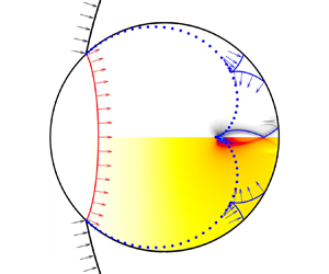
 $c$), and more details about the comparison between the numerical simulation results and theoretical results are presented in Appendix C. It is obvious that the shape and position of wave structures obtained by theoretical analysis almost coincide with the distribution of wave structures in the numerical results. Hence, this verifies the reliability and accuracy of the theoretical analysis in predicting the motion characteristics of the wave structures. Moreover, due to the strong stretched effect, a negative-pressure region is found near the intersection of two branches of the first reflected rarefaction wave. Meanwhile, the pressure behind the far branch of the first reflected rarefaction waves is quickly recovered because the subsequently emitted compression wavelets catch up with these two rarefaction wave branches.
3.2. The first convergence of the first reflected rarefaction wave
The first stage ends when the transmitted shock wave reaches the right pole of the water column at the time instant  $t_2$ (
 $t^* = 1.0$), and the second stage begins. At this moment, the transmitted shock wave is completely reflected, and two near branches of the reflected rarefaction wave on both sides of the central axis of the water column merge, forming a continuous converged rarefaction wave (Re-RW
 $_{IC}$). The analytical schematic is presented in figure 12(
 $a$), which demonstrates the first reflected rarefaction wave evolution. It is observed that the intersection points of Re-RW
 $_{II}$ and Re-RW
 $_{I}$ move along the envelope of the one-time reflected rays from time
  $t_2$ to
  $t_3$, and the continuous reflected rarefaction wave (Re-RW
 $_{IC}$) gradually focuses inside the water column. When Re-RW
 $_{IC}$ completely focuses, the two branches of the far-branch rarefaction wave meet and form a continuous diverged rarefaction (Re-RW
 $_{IIC}$).

Figure 12. ( $a$) Schematic diagram of the first reflected expansion wave propagation from
  $t_2$ (
 $t^* = 1.0$) to
  $t_3$ (
 $t^* = 1.2698$); (
 $b$) schematic diagram of ray analysis for the focusing of the one-time reflected rays.
Previous studies (Sembian et al. Reference Sembian, Liverts, Tillmark and Apazidis2016; Xiang & Wang Reference Xiang and Wang2017; Wu et al. Reference Wu, Xiang and Wang2018; Biasiori-Poulanges & El-Rabii Reference Biasiori-Poulanges and El-Rabii2021) have found that the complete focus of the reflected rarefaction wave decreases the water pressure rapidly, and the maximum negative pressure inside the water column reaches approximately  $-$10 MPa at the complete focus instant. The pressure distributions along the centre axis of the water column, just before and after the complete focus instant, are presented in figure 13, and it can be seen that a similar focusing pressure (
 $-$10 MPa) is obtained in the present study. This extremely negative pressure has far exceeded the cavitation threshold pressure of
  $-$2.3 MPa of unpurified water reported by Sembian et al. (Reference Sembian, Liverts, Tillmark and Apazidis2016). Therefore, the region inside the water near the focus point has a high probability of capturing the cavitation phenomenon. Hence, the focus point of the first reflected rarefaction wave is called the cavitation kernel point in the present study, denoted as
  $P_{cav}$. Combined with figure 12(
 $b$),
$b$),  $P_{cav}$ is also the left limiting position of the one-time reflected rays that intersect with the central axis of the water column.

Figure 13. The pressure distribution along the centre axis of the water column, just before and after the complete focus instant, for the interaction between the cylindrical converged shock and the water column.
The position of  $P_{cav}$ can be obtained theoretically according to the ray analysis (Obreschkow et al. Reference Obreschkow, Dorsaz, Kobel, de Bosset, Tinguely, Field and Farhat2011; Wu et al. Reference Wu, Xiang and Wang2018; Biasiori-Poulanges & El-Rabii Reference Biasiori-Poulanges and El-Rabii2021) considering the planar incident shock wave or flat rigid surface. Here, we present the case analysis considering the curved, cylindrical, incident shock wave.
Some rays emitted by the contact point whose contact angle is less than the critical contact angle  $\theta _{cr}$ are presented in figure 12(
 $b$). In order to ensure that the one-time reflected rays can intersect with the horizontal central axis, the emission angle
  $\alpha _\theta$ and the contact angle
  $\theta$ will satisfy
  $4{\alpha _\theta } + \theta > 180^\circ$. Selecting an arbitrary ray (the black solid lines) for analysis, the intersection points of the one-time reflected part of this ray with the column surface and the horizontal central axis are
  $E_\theta$ and
  $F_\theta$, respectively. And the distance
  $\lambda _\theta$ from
  $F_\theta$ to the column centre can be expressed as follows:
 \begin{equation} {\lambda_\theta } =
\frac{{\sin {\beta_\theta }}}{\sin {\psi_\theta }}{R_D} =
\frac{{{R_D}}}{{\sin \theta \sin {\alpha_\theta }(
{4\cos {\alpha_\theta } - {1 /\cos \alpha_\theta}} ) + \cos
\theta ( {3 - 4\cos ^2{\alpha_\theta }} )}}.
\end{equation}
\begin{equation} {\lambda_\theta } =
\frac{{\sin {\beta_\theta }}}{\sin {\psi_\theta }}{R_D} =
\frac{{{R_D}}}{{\sin \theta \sin {\alpha_\theta }(
{4\cos {\alpha_\theta } - {1 /\cos \alpha_\theta}} ) + \cos
\theta ( {3 - 4\cos ^2{\alpha_\theta }} )}}.
\end{equation}
After substituting (3.6) into (3.11) and simplifying, the expression of distance  $\lambda _\theta$ can be rewritten as follows:
 \begin{equation} {\lambda_\theta } = \frac{{{R_D}}}{{{F_1}( \theta ) - {F_2}( \theta ) + {F_3}( \theta )}}, \end{equation}
where,  ${F_1}( \theta )$,
  ${F_2}( \theta )$ and
  ${F_3}( \theta )$ are shown as
 $$\begin{gather} {F_1}( \theta ) = \frac{{4\kappa ( {\omega \,{-}\, 1} ){{\sin }^2}\theta }}{{\sqrt {1 + {{( {\omega \,{-}\, 1} )}^2} + 2( {\omega \,{-}\, 1} )\cos \theta } {M_\theta }}}\sqrt {1 - \frac{{{\kappa^2}{{( {\omega - 1} )}^2} \sin^2\theta }}{{[ {1 + {{( {\omega \,{-}\, 1} )}^2} + 2( {\omega \,{-}\, 1} )\cos \theta } ]{M_\theta }^2}}}, \end{gather}$$
 $$\begin{gather} {F_2}( \theta ) = \frac{{{M_\theta }\sqrt {1 + {{( {\omega \,{-}\, 1} )}^2} + 2( {\omega \,{-}\, 1} )\cos \theta } }}{{\kappa ( {\omega - 1} )}}\sqrt {1 \,{-}\, \frac{{{\kappa^2}{{( {\omega \,{-}\, 1} )}^2}{{\sin }^2}\theta }}{{[ {1 + {{( {\omega \,{-}\, 1} )}^2} + 2( {\omega \,{-}\, 1} )\cos \theta }]{M_\theta }^2}}}, \end{gather}$$
 $$\begin{gather} {F_3}( \theta ) = 3\cos \theta - \frac{{4{\kappa^2}{{( {\omega - 1} )}^2}\sin^2\theta \cos \theta }}{{[ {1 + {{( {\omega - 1} )}^2} + 2( {\omega - 1} )\cos \theta } ]{M_\theta }^2}}. \end{gather}$$
A maximum limiting value of  $\lambda _\theta$ exists. Accordingly, the position of
  $P_{cav}$, as well as the focus point of the one-time reflected rays, is obtained, which has the following expression:
 \begin{equation} \frac{{{\lambda_{max}}}}{{{R_D}}} = \lim_{\theta \to 0} \frac{{{\lambda_\theta }}}{{{R_D}}} = \frac{1}{{\displaystyle\lim_{\theta \to 0} {F_1}( \theta ) - \lim_{\theta \to 0} {F_2}( \theta ) + \lim_{\theta \to 0} {F_3}( \theta )}} = \frac{\kappa }{{3\kappa - {M_0}{f_s}}}, \end{equation}
where  ${f_s} = {\omega /(\omega - 1)}$ is the function characterising the effect of shock wave shapes in the case of the cylindrical converged incident shock wave.
The above expression has indicated that the relative distance from the cavitation kernel point  $P_{cav}$ to the column centre is determined by three dimensionless parameters: the shock Mach number
  $M_0$, the radius ratio
  $\omega$ between the cylindrical converged shock wave and the water column and the sound-speed ratio
  $\kappa$ between the water and the air. If the radius ratio tends to the infinite, the cylindrical converged shock wave degenerates into a planar one. Here, we define a new dimensionless parameter
  $n = \kappa /{M_0}$, which represents the ratio of the wave speed between the transmitted shock wave and the incident shock wave. The distance
  $x_f$ from the focus point
  $P_{cav}$ to the centre of the water column can be written as
 \begin{equation} {x_f} = \frac{n}{{3n - 1}}{R_D}, \end{equation}
which is then identical to the expression reported by Biasiori-Poulanges & El-Rabii (Reference Biasiori-Poulanges and El-Rabii2021). In other words, the theoretical analysis derived in this paper is universal for different incident shock wave shapes.
3.3. The second convergence of the second reflected waves
When Re-RW $_{IC}$ completely focuses, the continuous diverged rarefaction wave (Re-RW
 $_{IIC}$) propagates upstream of the water column and is reflected by the column surface, forming the second reflected compression wave (Re
 $_2$-CW) and the second reflected rarefaction wave (Re
 $_2$-RW). Due to the specific column surface, the one branch of the second reflected wave (Re
 $_2$-CW) firstly focuses on the central axis of the water column,
  $P_{tran}$, causing a high-pressure region whose maximum pressure reaches more than 60 times the initial pressure, as shown in figure 7(
 $k$). After an extremely short time, the two symmetrical reflected rarefaction waves (Re
 $_2$-RW), located on the upper and lower sides of Re
 $_2$-CW, merge and cause a rapid decrease in the local pressure. The pressure distribution along the centre axis of the water column at six different time instants, before and after the focus of Re
 $_2$-CW, is shown in figure 14. Obviously, the maximum pressure in the high-pressure region increases rapidly as the focus process continues before the complete focussing of Re
 $_2$-CW. After that, a significant negative-pressure region appears inside the water column, and the maximum pressure in the high-pressure region decreases rapidly and then disappears.

Figure 14. The pressure distribution along the centre axis of the water column at six different time instants for the interaction between the cylindrical converged shock and the water column.
The evolution characteristics of the second reflected wave from  $t_4$ (
 $t^* = 2.0$) to
  $t_5$ (
 $t^* = 2.326$) based on the ray analysis are shown in figure 15(
 $a$). Due to the different properties of the two branches of the second reflected wave, the liquid near
  $P_{tran}$ undergoes a violent pressure oscillation in a short time interval. The highly transient characteristics of liquid pressure have great significance in the biomedical field, which is a valuable measure to remove diseased tissue. Similar to the derivation of
  $P_{cav}$, the specific position of
  $P_{tran}$ can be obtained by the ray analysis. A schematic diagram of rays emitted from some contact points when Re
 $_2$-CW focuses is shown in figure 15(
 $b$), selecting an arbitrary ray (the black lines) for further analysis. Denoting the intersection points of the two-time reflected part of this ray with the column surface and the central axis of the water column as
  $E_{\theta 2}$ and
  $F_{\theta 2}$, respectively, with the distance from
  $F_{\theta 2}$ to
  $C$ being
  $\delta _{\theta }$,
 \begin{equation} {\delta_\theta } = \frac{{\sin {\beta_\theta }}}{{\sin ({\rm \pi} - 5{\beta_\theta } + \theta )}}{R_D} = \frac{{\cos {\alpha_\theta }}}{{\cos ( {5{\alpha_\theta } + \theta } )}}{R_D}. \end{equation}
Figure 15. ( $a$) Schematic diagram of the second reflected wave propagation from
  $t_4$ (
 $t^* = 2.0$) to
  $t_5$ (
 $t^* = 2.326$) and schematic diagram of shapes and positions of the reflected waves at time
  $t_5$; (
 $b$) schematic diagram of ray analysis for the intersection point between the reflected rays, with two-time reflection, and the central axis of the water column.
After substituting (3.6) into (3.18) and simplifying, the minimum distance of  $\delta _\theta$ can be obtained as
  $\delta _{min}$, which has the following expression:
 \begin{align} \frac{{{\delta_{min}}}}{{{R_D}}} &= \lim_{\theta \to 0} \left[ {\frac{{\cos {\alpha_\theta }}}{{( {16\cos^4{\alpha_\theta } - 20\cos^2{\alpha_\theta } + 5} )\cos {\alpha_\theta }\cos \theta - ( {16\cos^4{\alpha_\theta } - 12\cos ^2{\alpha_\theta } + 1} )\sin {\alpha_\theta }\sin \theta }}} \right]\nonumber\\ &= \frac{\kappa }{{5\kappa - {M_0}{f_s}}}. \end{align}
Moreover, to ensure that the two-time reflected rays can intersect with the horizontal central axis before it is reflected from the column surface, the emission angle  $\alpha _\theta$ and the contact angle
  $\theta$ will satisfy:
  $6{\alpha _\theta } + \theta < {360^ \circ }$. It is easy to find that, as the reflection time increases, the maximum contact angle of rays participating in the focus process gradually decreases. This means that fewer rays participate in the focusing process with the interaction process continuing, which makes the reflected wave and focus intensity weaker and weaker.
Similar to the transmitted shock wave and the first reflected rarefaction wave, the second reflected waves also reflect on the column surface, forming the third reflected compression wave, figure 15( $a$), which will focus inside the water column causing a high-pressure region. As the interaction continues, the high-pressure and low-pressure areas appear alternately at different positions on the centreline. Their analysis procedure is similar to the focusing of the first reflected expansion wave and the second reflected compression wave. The following expression gives a general formula of the distance from the focusing point
  $x_{f,N}$ of the
  $N$ times reflected wave to the column centre:
 \begin{equation} {\frac{{{x_{f,N}}}}{{{R_D}}} = \frac{\kappa }{{( {2N + 1} )\kappa - {M_0}{\,f_s}}}} ,\quad {N = 1,2,3, \ldots }. \end{equation}
However, the intensity of these waves, with three times or more reflection, has been dramatically reduced compared with the intensity of the transmitted shock wave, the first reflected rarefaction wave and the second reflected wave. Therefore, we will not elaborate further in the present study.
4. The effect of incident shock wave shapes and intensities
In addition to converged shock waves, diverged shock waves also widely interact with the gas–liquid interface in nature, industrial production and scientific research, such as the interaction of a blast wave with a droplet. The derivation for the interaction of a diverged cylindrical shock wave with a water column, figure 16, is similar to that of a converged cylindrical shock wave with a water column, which is introduced in § 3. Again, the initial shock wave Mach number  $M_0 =2.4$ and radius ratio
  $\omega = 4.0$ of the diverged cylindrical shock are chosen in the following analysis, and (3.1) and (3.2) for the interaction between the diverged shock and the water column can be rewritten as the following expressions:
 $$\begin{gather} {R_\theta } = {R_D}\sqrt {1 + {{( {\omega + 1} )}^2} - 2( {\omega + 1} )\cos \theta}, \end{gather}$$
 $$\begin{gather}\sin \chi = \frac{{( {\omega + 1} )\sin \theta }}{{\sqrt {1 + {{( {\omega + 1} )}^2} - 2( {\omega + 1} )\cos \theta } }}. \end{gather}$$
Figure 16. Schematic diagram of the interaction between the cylindrical diverged shock wave and the water column.
The critical contact angle  $\theta _{cr}$, when the transmitted shock wave just detaches from the incident diverged shock wave and the reflected shock wave, can be obtained as follows:
 \begin{equation} \frac{{\sqrt {1 + {{( {\omega + 1} )}^2} - 2( {\omega + 1} )\cos {\theta_{cr}}} }}{{( {\omega + 1} )\sin {\theta _{cr}}}} = \frac{{{c_{l,0}}}}{{{M_{\theta cr}}{c_{g,0}}}}. \end{equation}
In the case of  $M_0 =2.4$, the value of
  $\theta_{cr}$ for the diverged shock wave (
 $\omega = 4.0$) is 28.3
 $^\circ$ compared with
  $\theta _{cr} = 44.9^\circ$ for the converged shock wave (
 $\omega = 4.0$) and
  $\theta _{cr} = 35.1^\circ$ for the planar shock wave. The critical contact angle is compared in table 1 with the analytical and numerical results of the three configurations at different incident shock wave intensities and shapes. The simulation results agree with the analytical values. Meanwhile, compared with the interaction between the planar shock wave and the water column, the converged shock wave will delay the percussive behaviour of the transmitted shock wave, while the diverged shock wave will accelerate the appearance of this phenomenon. Similarly, the time
  $t_\theta$, which represents the time of contact point moving from the left pole of the water column to
  $P_\theta$, and the emission angle
  $\alpha _\theta$ at
  $P_\theta$ can be rewritten as follows:
 $$\begin{gather} {t_\theta } = \int_0^\theta {\frac{{( {\omega + 1} )\sin \xi{R_D}}}{{\sqrt {1 + {{( {\omega + 1} )}^2} - 2( {\omega + 1} )\cos \xi } {M_\xi }{c_{g,0}}}}\,{\rm{d}}\xi }, \end{gather}$$
 $$\begin{gather}\cos {\alpha_\theta } == \frac{{{c_{l,0}}}}{{{R_D}}}{t'_\theta } = \frac{\kappa }{{{M_\theta }}}\frac{{( {\omega + 1} )\sin \theta }}{{\sqrt {1 + {{( {\omega + 1} )}^2} - 2( {\omega + 1} )\cos \theta } }}. \end{gather}$$
Table 1. The critical contact angle  $\theta_{cr}$ values at different incident shock wave intensities and shapes.

Further, the location of the cavitation kernel point  $P_{cav}$ for a diverged shock interacting with a water column can be obtained by the ray analysis, and the distance from
  $P_{cav}$ to the water column centre
  $C$ is also denoted as
  $\lambda _{max}$
 \begin{equation} \frac{{{\lambda_{max}}}}{{{R_D}}} = \lim_{\theta \to 0} \frac{{{\lambda_\theta }}}{{{R_D}}} = \frac{\kappa }{{3\kappa - {M_0}{f_s}}}, \end{equation}
where  ${f_s} = {\omega /(\omega + 1)}$ is the function characterising the effect of shock wave shapes in the case of the cylindrical diverged incident shock wave.
Hence, considering (3.16), (4.6) and the formula for the interaction of the planar shock with a water column reported by Biasiori-Poulanges & El-Rabii (Reference Biasiori-Poulanges and El-Rabii2021), the function  $f_s$ characterising the effect of shock wave shapes can be rewritten in a unified form, that is
  ${f_s} = {\omega / (\omega - \varepsilon )}$. Here,
  $\varepsilon$ represents the types of incident shock shape (
 $-$1 represents the diverged shock, 0 represents the planar shock and 1 represents the converged shock). It can be found that the factors affecting the relative position of
  $P_{cav}$ can be divided into two parts. One part is the physical parameter, including property parameters of the two-phase system that affects the value of
  $\kappa$ and the initial strength of the incident shock wave that affects the value of
  $M_0$. Another part is the geometrical parameter which affects the value of the initial radius ratio
  $\omega$ if the curved shock wave has a cylindrical shape. A detailed analysis will be introduced in our further works when the shape of the curved shock wave is not as perfect as that of a cylindrical shock wave. Figure 17 presents the position of
  $P_{cav}$ for theoretical analysis of three incident shock wave shapes and three incident shock wave intensities varying with the dimensionless radius
  $\omega$. It can be found that the position of
  $P_{cav}$, in the case of the converged shock, will be obviously offset with the increase of the incident shock wave curvature
  ${1 /\omega }$, while its offset direction is opposite to that in the case of the diverged shock. Therefore, we can use a weaker converged shock to obtain the same focus point of the reflected rarefaction wave compared with the cases of the planar shock wave.

Figure 17. The position of  $P_{cav}$ for theoretical analysis for three incident shock wave shapes and three incident shock wave intensities varies with the dimensionless radius
  $\omega$.
The comparison of the numerical result at  $M_0 = 2.4$ for three different shapes of the incident shock wave is shown in figure 18. It can be found that the converged shock wave can delay the reflection transition of the incident shock wave from the regular reflection to the irregular Mach reflection, while the diverged shock wave can promote this process, as shown in figure 18(
 $b$). The pressure contours inside the water column for three different shapes of incident shock waves at their respective focus instants are shown in figure 18(
 $c$). The minimum pressure–time curves inside the water column for three different types of incident shock waves are shown in figure 19. It is noticed that the converged shock wave can significantly enhance the phenomenon of the negative pressure induced by the focus of the reflected rarefaction wave. In contrast, the diverged shock can observably restrain this negative-pressure phenomenon. In other words, for a certain purity of water, a maximum probability of cavitation exists in the interactions of the converged shock wave with a water column and a minimum probability of cavitation exists in the interactions of the diverged shock wave with a water column compared with the interactions of the planar shock wave with a water column. The main reason is that the larger critical angle makes the envelope of the transmitted shock wave have a larger ray density and brings a significant negative pressure. Similarly, the pressure oscillation (the difference between the maximum and minimum pressure) caused by the focus of the second reflected wave (Re
 $_2$-EW and Re
 $_2$-CW) is more apparent in the case of the converged shock wave, figure 19.

Figure 18. The comparison of the numerical results of the interaction between the shock wave and a water column,  $M_0 =2.4$, for three different types of the shape of the incident shock wave (1 represents the diverged shock wave, 2 represents the planar shock wave and 3 represents the converged shock wave).

Figure 19. The evolution of the minimum and maximum pressures inside the water column over time for three incident shock wave shapes,  $M_0 = 2.4$.
However, by observing figure 18( $d$), it can be found that the negative pressure inside the water column, caused by the second reflected rarefaction wave, is much more significant in the case of the diverged shock wave than that in the case of the converged shock wave. It is worth noting that the focus of Re
 $_2$-CW would not generate a sharp high-pressure peak in the case of the diverged shock wave and the planar shock wave, which appears in the case of the converged shock wave. The main reason is that, as the interaction continues, the intensity of the incident shock wave gradually increases in the case of the converged shock wave. Hence, the pressure behind the reflected rarefaction recovery is quicker than in the other two cases. Moreover, figure 19 also shows that the time required for the reflected rarefaction wave to focus completely is the lowest under the converged shock wave, while it reaches the maximum under the diverged shock wave. In conclusion, the converged shock wave can significantly enhance the probability of cavitation inside the water column and simultaneously shorten the distance from the focus point
  $P_{cav}$ to the column centre.
Previous studies in interactions of the planar shock wave with a water column (Sembian et al. Reference Sembian, Liverts, Tillmark and Apazidis2016; Xiang & Wang Reference Xiang and Wang2017; Biasiori-Poulanges & El-Rabii Reference Biasiori-Poulanges and El-Rabii2021) have shown that, with the increase of the incident shock wave intensity, there is a stronger negative-pressure effect caused by the first reflected rarefaction wave and a greater possibility of cavitation. In this section, we will determine how the initial shock wave intensity of different shapes of the incident curved shock wave influences the interaction process.
Figure 20( $a$) presents the minimum pressure
  $p_{min}$ during the focus of Re-RW
 $_{IC}$ for three incident shock wave shapes varying with shock wave intensity in the range of 1.2–4.5. A few trends stand out. One is that
  $p_{min}$ decreases rapidly as the shock intensity increases, and
  $p_{min}$ is always negative for all shock wave intensities. Additionally, the minimum pressure induced by the converged shock wave is always lower than that induced by the planar shock wave and the diverged shock wave, and this phenomenon becomes apparent at a higher shock wave intensity. In addition, the cavitation threshold pressure obtained from Sembian et al. (Reference Sembian, Liverts, Tillmark and Apazidis2016) is added in figure 20(
 $a$). It can be found that
  $p_{min}$ is supposed to exceed the cavitation threshold if the shock wave intensity is large enough. In other words, the stronger the incident shock wave intensity, the higher the cavitation possibility. Because the focus pressure is the lowest in the case of the converged shock wave, the converged shock wave can significantly enhance the cavitation possibility. The comparison of the position of
  $P_{cav}$ (
 $p_{minp}$) between theoretical analysis and numerical simulations for different incident shock wave shapes is shown in figure 20(
 $b$). It can be seen that, no matter what shape the incident shock wave is, the distance from
  $P_{cav}$ (
 $p_{minp}$) to the column centre
  $C$ increases as the shock wave intensity increases both in theoretical analysis and numerical simulations. In addition, compared with cases of the planar shock wave, an obvious left shift, decreasing the distance, is found in cases of the diverged shock wave, while a considerable right shift, increasing the distance, is found in cases of the converged shock wave. The numerical simulations show a similar trend to the theoretical analysis, although it is worth noticing that the theoretical focus point of the first reflected rarefaction wave
  $P_{cav}$ does not coincide with the minimum pressure point
  $p_{minp}$ in the numerical results, also presented by Biasiori-Poulanges & El-Rabii (Reference Biasiori-Poulanges and El-Rabii2021). This deviation between the theoretical analysis and numerical simulations is mainly caused by the assumption of the infinitely thin wave structures in the theoretical analysis. However, this assumption of discontinuity in mathematics does not exist in numerical simulations and experiments. Hence, if a higher prediction accuracy of the theoretical analysis is expected, the effect of wave width must be considered, but it is still hard to achieve in a short time. To this end, a balanced approach, which means the assumption of the infinitely thin wave structures is kept in the theoretical analysis, but the effect of grid size on predicting the position of the focusing point is considered, is used to verify our explanation as also shown in figure 20(
 $b$). It can be found that the deviation between theoretical results and numerical simulations decreases significantly if the effect of grid size is considered. Of course, the velocity estimation of the transmitted shock wave will also lead to a difference in the
  $P_{cav}$ position between the theoretical analysis and numerical simulations. Nonetheless, the theoretical results obtained in the present study still have a high accuracy in predicting the focus of reflected waves and the region with high cavitation possibility inside the water column.

Figure 20. ( $a$) The minimum pressure
  $p_{min}$ during the focusing of Re-RW
 $_{IC}$ for three incident shock wave shapes varies with shock wave intensity. (
 $b$) The focus point position for theoretical prediction (
 $P_{cav}$) and numerical simulation (
 $p_{minp}$) for three incident shock wave shapes varies with shock wave intensity.
5. Conclusion
In this paper, we examined the early stage of the interaction of the curved shock wave with a cylindrical water column emphasising the analysis of waves that are converging. The study was conducted using the ray analysis method complemented by numerical simulations.
The spatio-temporal evolution and interaction of the complicated waves inside the water column have been detailed when the cylindrical converged, cylindrical diverged and planar shock waves are considered. The transmitted shock wave is generated inside the water column immediately after the impact of the shock wave. When the contact angle  $\theta$ is larger than the critical value
  $\theta {cr}$, the transmitted shock wave will detach from the incident shock wave, forming the precursor shock wave. The value of
  $\theta {cr}$ is determined by the incident shock wave intensity, the sound-speed ratio of the two phases and the shapes of the incident shock. Meanwhile, although there are countless rays on the same compression wavelet, only one ray, whose emission angle
  $\alpha _\theta$ satisfies (3.6), will affect the envelope of compression wavelets. After the detachment, the precursor shock wave propagates and transiently reflects from the column surface, generating a series of rarefaction waves. The focus of the reflected rarefaction wave can induce negative-pressure regions, where a higher probability of cavitation exists if the wave strength is high enough. In addition, a highly transient pressure oscillation is observed near the focus region of the second reflected wave, whose two branches have opposite properties. Based on the ray analysis, the positions of the focusing points of the first reflected rarefaction wave and the second reflected wave are derived, as determined by the dimensionless sound speed
  $\kappa$, the initial shock wave intensity
  $M_0$ and the dimensionless function
  $f_s$ characterising the effect of shock wave shapes.
The present study also investigates the effects of the initial shock wave intensity and the shapes of the incident shock wave. It is found that, due to having a larger critical detachment angle  $\theta {cr}$ that will bring a larger ray density to the compression wavelet envelope, the converged shock wave envelope induces a stronger negative pressure and a stronger pressure oscillation inside the water column, while the diverged shock wave, having a smaller detachment critical angle, weakens these phenomena. However, due to a rapid pressure recovery after the reflected rarefaction wave, the diverged shock wave can induce a significant secondary negative-pressure effect when the second reflected wave focuses inside the water column, compared with the other two shapes of the incident shock wave. In addition, the converged shock wave can shorten the distances from the focus points to the column centre, enhancing the probability of cavitation inside the water column. It is undoubtedly the case that the diverged shock wave increases these distances and weakens the cavitation probability. Based on the above analysis, the wave structure evolution mechanism and essential influencing factors can contribute to practical applications, such as fuel droplet atomisation under the interaction of a cellular detonation wave. Future work will further investigate the cavitation behaviours induced by the rarefaction waves during the curved shock wave and the droplet interactions.
Funding
This work is partially supported by the National Natural Science Foundation of China (grant nos 91952205, 12002039) and the National Science and Technology Major Project of China (grant nos 2017-I-0004-0004, 2017-III-0005-0030), respectively.
Declaration of interests
The authors report no conflict of interest.
Appendix A
In this appendix, to verify the reliability of the CCW theory, the comparison of dimensionless parameters of the cylindrical shock wave, varying with different shock radii, between the CCW theory and numerical simulation is presented in figure 21. Here,  $V_{ms}$ and
  $p_s$ represent the velocity magnitude and pressure at the wavefront of the cylindrical shock wave. Subscript 0 indicates that the cylindrical shock wave radius equals
  $R_0$. It is found that the CCW theory can better predict the convergence of the cylindrical shock wave, although the deviation of the cylindrical shock intensity obtained by the CCW theory and the numerical simulation is observed. Actually, to avoid this deviation (Zhang Reference Zhang2017), we can make the shock intensity at the
  $R = R_0$ equal to our desired value by constantly adjusting the initial cylindrical shock intensity at
  $R_{int}$ (
 $R_{int}$ is much bigger than
  $R_0$ in the case of the converged shock wave, and
  $R_{int}$ is much smaller than
  $R_0$ in the case of the diverged shock wave).

Figure 21. The comparison of dimensionless parameters of the cylindrical shock wave varying with different shock radii between the CCW theory and numerical simulation.
Appendix B
In this appendix, the grid independence verification is performed, taking the case of the cylindrical shock wave interacting with a water column. Here, the incident shock wave intensity  $M_0$ is taken as 2.4, and the dimensionless incident shock wave radius
  $\omega$ is taken as 4.0. The grid sensitivity is analysed by choosing three different grid resolutions: 5.8 (Grid-I), 13.0 (Grid-II) and 23.0 million cells (Grid-III). The grid cells per the water column diameter correspond to 800, 1200 and 1600, respectively.
The pressure contours and numerical schlieren contours for three different grid resolutions at the same instant are shown in figure 22. A similar distribution is noticed for pressure contours and numerical schlieren contours of the three different grid levels. As the grid resolution is enhanced, the captured flow field structures, including the shock wave structures and two-phase interfaces, become sharper. The extracted pressure profiles along the symmetrical axis of the water column under three different grid resolutions are shown in figure 23, where the abscissa axis is normalised by  $R_D$. The three pressure curves with different grid resolutions are basically overlapping, and the pressure discontinuity caused by the reflected rarefaction wave is sharpened with the increase of grid resolution. Slight deviations from the pressure distribution are observed behind the reflected rarefaction wave in Grid-I due to the low grid resolution, while the pressure distributions overlap well for the other two higher grid resolutions. Grid-II is finally chosen in the present study to balance the resolution of the flow field and the computational efficiency.

Figure 22. The numerical schlieren (top) and pressure (bottom) contours of the three different grid resolutions at  $t = 3.6$
  $\mathrm {\mu }$s,
  $\omega = 4.0$ and
  $M_0 = 2.4$.

Figure 23. Pressure distribution along the symmetrical axis of the water column under three different grid resolutions at  $t = 3.6$
  $\mathrm {\mu }$s,
  $\omega = 4.0$ and
  $M_0 = 2.4$.
Appendix C
The comparison of wave structure evolution characteristics between the numerical simulation (top side) and the theoretical result (bottom side) for the interaction between the cylindrical converged shock and the water column in the case of  $\omega = 4.0$ and
  $M_0 = 2.4$ is presented in this appendix in figure 24. It is easily found that the theoretical analysis method can perfectly reveal the spatio-temporal evolution of wave structures inside the shocked water column, although small offsets are captured when the shocked water column appears to have a slight deformation.

Figure 24. Comparison of the confined wave structure spatio-temporal dynamics theoretically predicted (bottom side) with numerical schlieren contour (top side) for the interaction between the cylindrical converged shock and the water column in the case of  $\omega = 4.0$ and
  $M_0 = 2.4$.


