


1. Introduction and motivation
The availability of reliable information about processes within and states of technical systems is essential for achieving the vision “Industry 4.0”, e.g., to enable predictive maintenance and digital twins [cf. e.g. Schirra et al. Reference Schirra, Martin, Vogel and Kirchner2018; Matt & Rauch Reference Matt, Rauch, Zsifkovits, Modrák and Matt2020]. In this context, the term “technical system” covers a wide range from entire (production) plants and machines to assemblies and their components, such as machine elements [cf. Pahl et al. Reference Pahl, Beitz, Feldhusen and Grote2007]. The demand for information results in additional requirements for these systems that exceed the ones characterizing their primary functions – system-specific process or state variables must be measured.
Depending on the individual branch of industry, the statistical average age of German machinery is between 12 and 18 years. In the USA, the statistical average age is around 10 years. However, from a technical point of view, the machines are even two to three years older than that due to the required development time [cf. Guerreiro et al. Reference Guerreiro, Lins, Sun, Schmitt, Hamrol, Ciszak, Legutko and Jurczyk2018]. Accordingly, it can be stated that many technical systems existing today – especially those with long life cycles – were not developed against today’s background. Consequently, these machines are unable to provide information about relevant process or state variables. Since replacing every outdated machine is barely realistic in short term and medium term, but also uneconomical, retrofitting of measurement functions comes to the fore.
Since new requirements are involved when retrofitting measuring functions into existing systems, the “Guideline Sensors for Industrie [sic] 4.0” of the German Engineering Federation emphasizes the importance of a solution-neutral discussion of potential measurands [cf. Fleischer et al. Reference Fleischer, Klee, Spohrer, Merz and Metten2018]. However, the question of potential measurands arises regardless of whether the integration of a measuring function is carried out in form of a retrofit or in the context of a new sensory development. In both cases, the aim is to obtain defined information.
The overall objective when integrating measuring functions is to provide reliable information about processes or states in (existing) technical systems effectively and efficiently. Against this background, this contribution presents an approach developed by Vorwerk-Handing (Reference Vorwerk-Handing2021) to systematically establish a relationship between a system-specific state or process variable to be determined and potential measurands. In the approach, physical effects are used and the (existing) technical system as well as its properties is taken into account, the latter in contrast to Helms, Schultheiss & Shea (Reference Helms, Schultheiss and Shea2013). Therefore, the fundamental approach of using physical effect catalogs is taken up and transferred to the considered context. To overcome the limitations identified in the application of the approach, a new catalog system – so-called multipole-based effect catalog system – was developed by Vorwerk-Handing (Reference Vorwerk-Handing2021) in order to provide a basis for the solution-neutral identification and discussion of potential measurands. In the following, a translated summary of the main research results of Vorwerk-Handing (Reference Vorwerk-Handing2021) and a presentation of research thematically connected to it is provided.
The remaining contribution is structured as follows: In Section 2, the relevant fundamentals of this contribution are outlined. In Section 3, the aims of this contribution but also its significance are described. The structure and approach for the multipole-based effect catalog system are explained in Section 4. In Section 5, a brief assessment of the results is described. The contribution ends with Section 6, which provides a conclusion and an outlook.
2. Fundamentals
In literature, the development of (retrofit) solutions for the integration of measuring functions into technical systems is oftentimes described in form of process models [cf. e.g. Fleischer et al. Reference Fleischer, Klee, Spohrer, Merz and Metten2018; Hausmann et al. Reference Hausmann, Breimann, Fett, Kraus, Schmitt, Welzbacher and Kirchner2023]. An essential step therein is typically the “definition of potential measurands”. This is due to the circumstance, that both – direct as well as indirect measurements – are in principle conceivable for measuring physical quantities in a technical system [cf. Regtien Reference Regtien2005; Bureau international des poids et mesures 2008]. Thus, to ensure a uniform understanding, a distinction is made in the following between the state or process variable to be determined and the actual measurand. The process or state variable to be determined is the actual target of the measurement and the subsequent evaluation of the obtained data [cf. e.g. Regtien Reference Regtien2005]. A measurand is defined, according to the Joint Committee for Guides in Metrology (JCGM), as the “quantity intended to be measured” and thus is the input variable of the sensor [cf. Bureau international des poids et mesures 2012].
In this section, the fundamentals for the methodical establishment of a relationship between a system-specific process or state variable to be determined and potential measurands are described. This includes not only the modeling of measurements based on physical effects but also physical effect catalogs as well as existing approaches for the multidisciplinary modeling of technical systems.
2.1. Modeling of measurements
Measurements, that is the acquisition and representation of physical quantities and the assignment of their corresponding values, are subject of the interdisciplinary field of metrology [cf. Bureau international des poids et mesures 2012]. The structure of an abstracted measurement system is shown in Figure 1, whereby the contents of this contribution are located in the measuring transducer.

Figure 1. Structure of an abstracted measurement system [translated from Czichos Reference Czichos2019].
Sensors change or convert a physical, chemical or biological measurand into an output signal – nowadays usually an electrical signal. Hence, a sensor can be defined as a device that receives the measurand as input and generates a conditioned electrical signal as output. [cf. e.g. Regtien Reference Regtien2005; Wilson Reference Wilson2005; Kalantar-zadeh & Fry Reference Kalantar-zadeh, Fry, Kalantar-zadeh and Fry2008].
Since a sensor in general changes a signal, a measurement can be considered as a recording of the effect
 $ {X}_1 $
of a cause
$ {X}_1 $
of a cause
 $ Y $
(measurand). The relationship between these two variables is built using physical effects and described by the function
$ Y $
(measurand). The relationship between these two variables is built using physical effects and described by the function
 $ h $
, cf. Figure 2. Besides these two variables, the function
$ h $
, cf. Figure 2. Besides these two variables, the function
 $ h $
typically includes other variables, such as design parameters, which are designated as
$ h $
typically includes other variables, such as design parameters, which are designated as
 $ {X}_2,{X}_3,\dots, {X}_{\mathrm{N}} $
. Influences not taken into account in the function
$ {X}_2,{X}_3,\dots, {X}_{\mathrm{N}} $
. Influences not taken into account in the function
 $ h $
or modeling imperfections, e.g. regarding the measuring object, its environment or the measuring device, cause uncertainty. [cf. Bureau international des poids et mesures 2008; Kreye, Goh & Newnes Reference Kreye, Goh and Newnes2011].
$ h $
or modeling imperfections, e.g. regarding the measuring object, its environment or the measuring device, cause uncertainty. [cf. Bureau international des poids et mesures 2008; Kreye, Goh & Newnes Reference Kreye, Goh and Newnes2011].
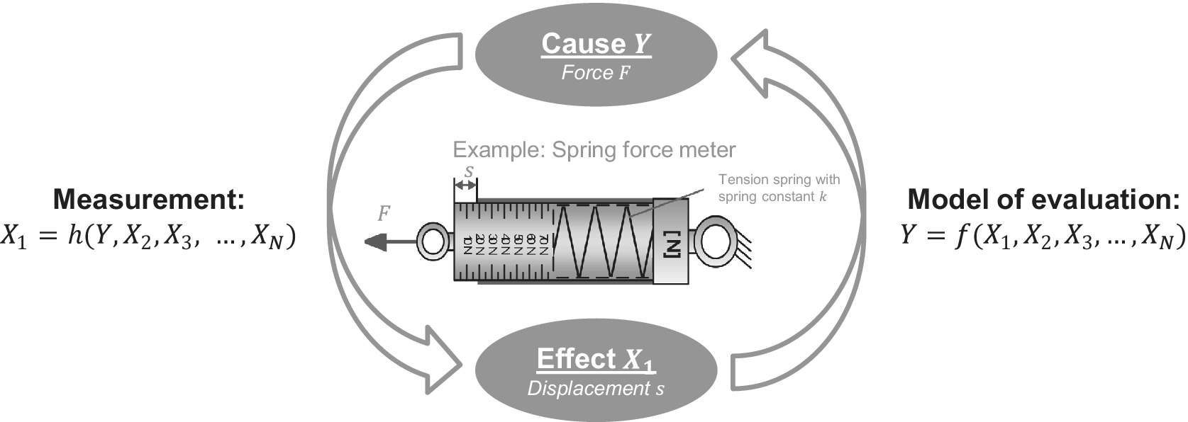
Figure 2. Development of a model of evaluation based on a cause–effect relationship [cf. Harder et al. Reference Harder, Gross, Vorwerk-Handing and Kirchner2021; based on Wilson Reference Wilson2005 and Weckenmann, Sommer & Siebert Reference Weckenmann, Sommer and Siebert2006].
The goal of a measurement is to conclude from the measured effect
 $ {X}_1 $
to the initial cause
$ {X}_1 $
to the initial cause
 $ Y $
. This is done via the so-called model of evaluation, which is described by the function
$ Y $
. This is done via the so-called model of evaluation, which is described by the function
 $ f $
[cf. Bureau international des poids et mesures 2008]. The function
$ f $
[cf. Bureau international des poids et mesures 2008]. The function
 $ f $
is obtained by rearranging the function
$ f $
is obtained by rearranging the function
 $ h $
according to the searched variable, the measurand
$ h $
according to the searched variable, the measurand
 $ Y $
.
$ Y $
.
2.2. Physical effects
The relationship between the input and output quantities of a technical system – in terms of its function – is established by physical, chemical and/or biological effects [cf. e.g. Pahl et al. Reference Pahl, Beitz, Feldhusen and Grote2007; Mokhtarian, Coatanéa & Paris Reference Mokhtarian, Coatanéa and Paris2017]. Accordingly, a function of a technical system can be described by means of the utilized effects. In mechanical engineering, the aforementioned relationship usually comes about as a result of a physical effect or the linkage of several physical effects [cf. e.g. Hansen & Andreasen Reference Hansen and Andreasen2002; Pahl et al. Reference Pahl, Beitz, Feldhusen and Grote2007; Stetter Reference Stetter2020].
A physical phenomenon or event is defined as physical effect, whereby the corresponding quantitative relationship between the involved physical quantities is referred to as physical law. Since physical effects enable the fulfillment of functions, their consideration represents an established approach when aiming for a function to be realized. The technical realization of a physical effect takes place through a geometric-material structure – so-called working geometry – in a defined environment, that is in the technical system. In this context, the link between physical effect and working geometry is referred to as the working interrelationship. The necessary conditions of a technical system to realize a physical effect can be described by the geometric, material and kinematic properties of the system. Figure 3 illustrates the different terms, using the example of a mechanical lever. [cf. Finkelstein, El-hami & Ginger Reference Finkelstein, El-hami and Ginger1998; Pahl et al. Reference Pahl, Beitz, Feldhusen and Grote2007; Stetter Reference Stetter2020].
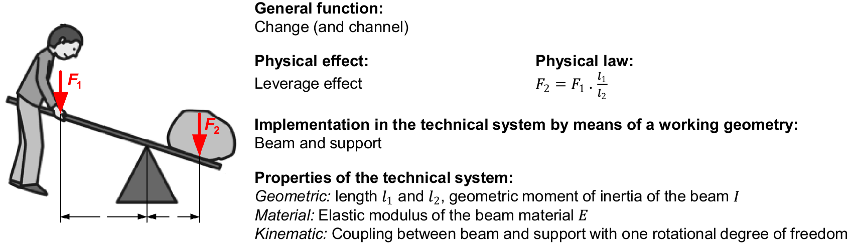
Figure 3. Realization of a function in a technical system based on a physical effect [translated from Vorwerk-Handing Reference Vorwerk-Handing2021].
2.3. Physical effect catalogs
For the development of technical systems, the availability of information at a specific point in time is an elementary prerequisite. However, a considerable proportion of (generally) acquired knowledge cannot be applied usefully, because it is generally not available or not available in a suitable form. This applies in particular to developers who permanently rely on physical, technological or material knowledge. As soon as the information available in the developers’ memory is no longer sufficient, access to externally stored knowledge or information is required [cf. Savransky Reference Savransky2000]. Therefore, design catalogs can be used as tools to improve the availability and utilization of existing knowledge and consequently as suitable means for better solutions. [cf. e.g. Verein Deutscher Ingenieure 1982; Koller Reference Koller1998; Helms et al. Reference Helms, Schultheiss and Shea2013; Ehrlenspiel & Meerkamm Reference Ehrlenspiel and Meerkamm2017].
According to VDI 2222 – Sheet 2, the generic term design catalog covers information and knowledge repositories that are tailored to the methodical development of technical systems in terms of their content, access features and structure. Design catalogs are characterized by extensive completeness, access features as well as a clear system and structure. Design catalogs are further distinguished into three types:
-
• object catalogs,
-
• operation catalogs and
-
• solution catalogs [cf. Verein Deutscher Ingenieure 1982].
Since object catalogs contain task-independent information necessary for development, especially from the field of physics, they come to the fore at this point. Object catalogs that contain information about physical effects are designated as physical effect catalogs. These catalogs differ from mere collections of physical effects, e.g., the one from Young & Freedman (Reference Young and Freedman2016), in terms of access features. [cf. Verein Deutscher Ingenieure, 1982].
Since physical effects generally establish a relationship between two physical quantities, effect catalogs are structured accordingly, based on the cause–effect principle of the involved quantities [cf. e.g. Koller Reference Koller1998; Roth Reference Roth2000; Ehrlenspiel & Meerkamm Reference Ehrlenspiel and Meerkamm2017]. Similar to the structure of design catalogs, physical effect catalogs consist of an outline section, a main content and an access section – including an appendix, if applicable. Depending on the number of physical quantities involved in the structuring of an effect catalog, a distinction is made between one-, two- or three-dimensional catalogs. The fundamental structure of effect catalogs and the distinctions introduced are illustrated in Figure 4.

Figure 4. Structure of physical effect catalogs with a one- or two-dimensional outline section [translated from Vorwerk-Handing Reference Vorwerk-Handing2021; based on Koller Reference Koller1998 and Roth Reference Roth2000].
The structure of existing effect catalogs as well as their respective inclusion in a procedure for the synthesis of principle solutions differs in detail depending on the author [cf. Helms et al. Reference Helms, Schultheiss and Shea2013]. The most widespread catalog systems are the one by Koller (Reference Koller1998) and the function variable matrix by Roth (Reference Roth2000). These two systems serve as references in the following.
At this point, it should be noted that besides analog catalog systems, there are also digital systems in the form of effect databases. An example of such a database is the one by Oxford Creativity Ltd. (n.d.) or the SAPPhIRE database by Srinivasan & Chakrabarti (Reference Srinivasan, Chakrabarti, Taura and Nagai2011). Effect databases are oftentimes referred to in the “Theory of Inventive Problem Solving” (TRIZ). Since it is not possible to derive generally valid statements from existing effect databases due to a lack of available information about their completeness as well as underlying structure and logic, their significance for this contribution is rated low and they are neglected in the following. In perspective, however, the computer-based implementation of the results of this contribution in the form of an effect database is conceivable and worthwhile.
2.4. Multidisciplinary modeling of technical systems
Mechatronic systems typically consist of a basic system, sensors, actuators and an information processing unit [cf. e.g. Verein Deutscher Ingenieure 2021]. Qualitative system models make it possible to structure such a system in a way that it is understandable for the developer and the inner relationships become apparent [cf. e.g. Mokhtarian et al. Reference Mokhtarian, Coatanéa and Paris2017]. On this basis, design variants can be developed. Furthermore, the qualitative modeling of the system enables the subsequent quantitative modeling of clearly defined and manageable subsystems in form of mathematical equations [Janschek Reference Janschek2012]. In general, two approaches can be used to model mechatronic systems:
-
• On the one hand, according to the “domain-specific design” described in the V‑model, they can be modeled from the point of view of the involved disciplines – mechanical, electrical and software engineering [cf. Verein Deutscher Ingenieure 2021].
-
• On the other hand, a domain-independent modeling of the entire system can be done [cf. Janschek Reference Janschek2012].
Since the former contradicts the cross-domain modeling required for a systematic identification of potential measurands, domain-independent multipole-based modeling is chosen. The structure of a multipole-based network model allows to obtain the physical topology of the considered system. This offers the possibility to modularize models – or the modeling process in general – on the basis of an explicit technical component assignment. In addition, the multipole-based modeling approach is also suitable for complex systems [cf. Janschek Reference Janschek2012].
In multipole-based modeling, systems with a multidisciplinary character are described uniformly on the basis of lumped parameter network elements and general energy conservation laws. The linkage of the spatially and functionally delimited network elements to an overall system model takes place via terminals, ports, respectively, based on power‑conservation interconnection laws (Kirchhoff’s laws). Based on the number of terminals, network elements are distinguished into two terminal or single ports, three terminal, four terminal or two ports or multiports, cf. Figure 5. [cf. e.g. Janschek Reference Janschek2012].

Figure 5. Overview of different types of lumped network elements [translated from Vorwerk-Handing Reference Vorwerk-Handing2021; based on Janschek Reference Janschek2012].
The basis of multipole-based modeling is the energy exchange between the network elements by means of a pair of conjugated generalized energy variables or terminal variables [cf. e.g. MacFarlane Reference MacFarlane1964; Wellstead Reference Wellstead1979; Janschek Reference Janschek2012]. These are defined as
-
• generalized effort variable
 $ e $
and
$ e $
and -
• generalized flow variable
$ f $
.


Examples of generalized effort variables are the velocity
 $ v $
or the electric voltage
$ v $
or the electric voltage
 $ U $
, whereas examples of generalized flow variables are the force
$ U $
, whereas examples of generalized flow variables are the force
 $ F $
or the electric current
$ F $
or the electric current
 $ I $
.Footnote
1 The product of the domain-specific effort and flow variable is power
$ I $
.Footnote
1 The product of the domain-specific effort and flow variable is power
 $ P(t) $
, cf. equation 1 [cf. e.g. MacFarlane Reference MacFarlane1964; Wellstead Reference Wellstead1979; Janschek Reference Janschek2012].
$ P(t) $
, cf. equation 1 [cf. e.g. MacFarlane Reference MacFarlane1964; Wellstead Reference Wellstead1979; Janschek Reference Janschek2012].
 $$ P(t):=e(t)\bullet f(t) $$
Since the pair of generalized energy variables describes the energy exchange, but not the energy stored within the system or element, these two quantities are not sufficient to describe the total energy of a system or element. The total energy in a closed system or element can be described by fundamental variables. Since energy, as a quantity-like physical state variable, cannot flow alone, it always requires an energy carrier. Each energy carrier in turn has a potential [cf. Wellstead Reference Wellstead1979]. The already introduced generalized energy variables
 $ e $
and
$ e $
and
 $ f $
are not dependent on the size of the system or a quantity in general. For this reason, they are designated as intensive state variables or intensity variables
$ f $
are not dependent on the size of the system or a quantity in general. For this reason, they are designated as intensive state variables or intensity variables
 $ {i}_j $
. Examples of intensive state variables are the force
$ {i}_j $
. Examples of intensive state variables are the force
 $ F $
, the electric current
$ F $
, the electric current
 $ I $
, the velocity
$ I $
, the velocity
 $ v $
or the electric voltage
$ v $
or the electric voltage
 $ U $
. In contrast, state variables that are dependent on the size of the considered system or generally a quantity are called extensive state variables
$ U $
. In contrast, state variables that are dependent on the size of the considered system or generally a quantity are called extensive state variables
 $ {q}_j $
. Examples of extensive state variables are the momentum
$ {q}_j $
. Examples of extensive state variables are the momentum
 $ p $
, the electric charge
$ p $
, the electric charge
 $ Q $
, the displacement
$ Q $
, the displacement
 $ s $
or the induction flux
$ s $
or the induction flux
 $ \varPhi $
. Intensive and extensive state variables are linked according to equation 2.
$ \varPhi $
. Intensive and extensive state variables are linked according to equation 2.
 $$ {i}_j:=\frac{d{q}_j}{dt} $$
According to Gibb’s fundamental form for equilibrium states, the energy change of a system is calculated according to equation 3.
 $$ \delta E=\sum \limits_j{i}_j\bullet \delta {q}_j $$
According to equation 3, the total energy of a system or an element results from the sum of the products of the two pairwise intensive and extensive state variables [cf. Wellstead Reference Wellstead1979]. Hence, within a physical domain, exactly four system variables can always be formed, two intensive variables and two extensive variables. The two intensive variables and extensive variables can further be distinguished based on their metrological properties:
-
• State variables, for whose determination only one point in space is required, are designated as P-variables (from Latin per – “through”) or single-point variables. They are denominated with the index P. Examples for P-variables are the force
$ F $
, the electric current
$ I $
, the momentum
$ p $
or the electric charge
$ Q $
. -
• State variables, for whose determination two points in space are required, are designated as T-variables (from Latin trans – “over”) or two-point variables. They are denominated with the index T. Examples for T-variables are the velocity
$ v $
, the electric voltage
$ U $
, the displacement
$ s $
or the induction flux
$ \varPhi $
.


The definitions and relationships described above are summarized in Table 1. The already mentioned examples from the domains of mechanics and electricity are taken up consistently in this table as well as in Table 2 and in Figure 6.
Table 1. Summary of system variables in the context of multipole-based modeling [translated from Vorwerk-Handing Reference Vorwerk-Handing2021; Janschek Reference Janschek2012]

Note:
P-variable ≙ one-point variable extensive state variable ≙ „quantity“
T-variable ≙ two-point variable intensive state variable ≙ „intensity“
Table 2. Overview of the constitutive laws for the linkage of system variables [translated from Vorwerk-Handing Reference Vorwerk-Handing2021]
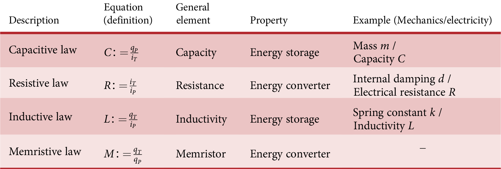

Figure 6. Overview of the system variables and their linkage by constitutive laws [based on Paynter Reference Paynter1961].
The introduced system variables are linked by two types of constitutive laws. The temporal relationship between intensive and extensive state variables has already been introduced in equation 2. The relationship between P- and T-variables is established via design parameters. These design parameters cause either storing (e.g., spring constant
 $ k $
or electric capacity
$ k $
or electric capacity
 $ C $
) or transforming (e.g., internal damping
$ C $
) or transforming (e.g., internal damping
 $ d $
or electrical resistance
$ d $
or electrical resistance
 $ R $
) properties on the systems’ level. The different constitutive laws are summarized in Table 2.
$ R $
) properties on the systems’ level. The different constitutive laws are summarized in Table 2.
An overview of the system variables, their laws of formation and their linkage by constitutive laws is shown in Figure 6. It apparent, starting from the primary variable
 $ X $
, that the other three system variables can be derived unambiguously, at least mathematically. In practice, however, it is not always trivial to set up the cross-domain analogy relationships in the correct way [cf. Janschek Reference Janschek2012].
$ X $
, that the other three system variables can be derived unambiguously, at least mathematically. In practice, however, it is not always trivial to set up the cross-domain analogy relationships in the correct way [cf. Janschek Reference Janschek2012].
3. Aims and significance
The integration of measurement functions into existing technical systems is one of the current challenges in mechanical engineering. This is of great importance and topicality, especially against the background of “Industry 4.0” and predictive maintenance. To avoid an early unfounded restriction of the solution space by a prefixation and thus impede innovative or promising solutions, the importance of a solution-neutral discussion of potential measurands is emphasized in literature [cf. e.g. Fleischer et al. Reference Fleischer, Klee, Spohrer, Merz and Metten2018]. Hence, the users’ creativity is stimulated, mental blocks are dissolved and innovative solutions are enhanced [cf. Zavbi & Duhovnik Reference Zavbi and Duhovnik2001; Srinivasan & Chakrabarti Reference Srinivasan, Chakrabarti, Taura and Nagai2011; Stetter Reference Stetter2020]. However, no systematic approach to establish relationships between a state or process variable to be determined and potential measurands, taking an existing system into account, could be found in literature [cf. Vorwerk-Handing Reference Vorwerk-Handing2021; Hausmann et al. Reference Hausmann, Breimann, Fett, Kraus, Schmitt, Welzbacher and Kirchner2023].
This chapter is structured as follows: In Section 3.1, potentials and limitations of existing effect catalogs are discussed. Based on the outcome of this discussion, the objective and research design are described in Section 3.2.
3.1. Potentials and limitations of existing effect catalogs
Since physical effects in general establish a relationship between different physical quantities, effect catalogs are used to systematically establish relationships between process or state variables to be determined and potential measurands. In the intended context, the application of existing effect catalogs is in principle permissible. However, the previously considered main representatives of analog effect catalogs, Koller (Reference Koller1998) and Roth (Reference Roth2000), were originally developed to find working principles for (sub-)functions to be realized [cf. Pahl et al. Reference Pahl, Beitz, Feldhusen and Grote2007]. Hence, the original purpose of these catalogs is to establish a relationship between a sought for effect and causes that could potentially be used for the intended purpose. As a result, there are two major limitations to the identification of cause–effect relationships by means of existing effect catalogs:
-
• Existing effect catalogs assume an effect to be realized. Due to the irreversibility of some physical effects, an inverse application of existing catalogs is not permissible.
-
• According to the original purpose of effect catalogs, a consideration of design information is not intended. With regard to the intended consideration of existing systems, it is stated that the inclusion of the design of an existing technical system is not sufficiently supported.
As a result, not all usable relationships between system-specific process or state variables and potential measurands can be mapped systematically using existing effect catalogs. Since the effect catalogs by Koller (Reference Koller1998) and Roth (Reference Roth2000) differ in particular in terms of structuring and content, more detailed restrictions were elaborated in Vorwerk-Handing (Reference Vorwerk-Handing2021).
3.2. Objective and research design
The main objective is the systematic establishment of relationships between a system‑specific process or state variable and potential measurands to realize a sought for measuring function. The technical system into which the measuring function is to be integrated is considered by modeling on the level of physical effects using an effect matrix and the associated effect catalog.
As basis for the conception and development of an effect matrix and the associated effect catalog, requirements and boundary conditions are collected and defined. The requirements are based on the analysis of the problem-related limitations of existing catalog systems and are completed in accordance with VDI 2222 – Sheet 2 [Verein Deutscher Ingenieure 1982]. To develop a catalog system that meets these requirements, Vorwerk-Handing (Reference Vorwerk-Handing2021) took up the fundamental idea of the effect catalogs by Koller (Reference Koller1998) and Roth (Reference Roth2000) and combined it with the fundamentals of multipole-based modeling. Thus, the chosen approach provides a basis for the systematic identification of potential measurands while taking an existing technical system into account.
4. Multipole-based effect catalog system
In order to systematically establish relationships between a system-specific process or state variable and potential measurands, a catalog system consisting of an effect matrix and an associated effect catalog was developed by Vorwerk-Handing (Reference Vorwerk-Handing2021). For the development of this catalog system, the fundamental idea of the catalog systems by Koller (Reference Koller1998) and Roth (Reference Roth2000) is taken up and combined with the fundamentals of multipole-based modeling. According to the intended purpose, a cause–effect perspective is consistently applied. This results in a physically and logically justified structure of the developed catalog system.
The overall objective of the developed catalog system is to establish relationships between a system‑specific process or state variable and potential measurands. This is achieved by linking several physical effects and thus forms a so‑called effect chain. Generalized relationships between a cause and a resulting effect are systematically built and mapped in the two-dimensional effect matrix. Information about the respective physical effects that establish these relationships is stored in the one-dimensional effect catalog.
To ensure that the generated effect chains are metrologically usable with respect to the accuracy that can be achieved with them, an uncertainty analysis has to be conducted. Since the focus in this contribution is on the multipole-based effect catalog system, the topic of uncertainty analysis is not included in this contribution. For a detailed description of the uncertainty analysis including various application examples, it is referred to Vorwerk-Handing, Welzbacher & Kirchner (Reference Vorwerk-Handing, Welzbacher and Kirchner2020) and Vorwerk-Handing (Reference Vorwerk-Handing2021).
This chapter is structured as follows: The two-dimensional effect matrix of the catalog system and its structuring are described in Section 4.1. The associated one-dimensional effect catalog is described in terms of its main content and access section in Section 4.2.
4.1. Effect matrix
The two-dimensional overview catalog of the catalog system is structured in the form of a matrix, designated as effect matrix, which is schematically shown in Figure 7. The matrix lists the causes in columns and the resulting effects in rows. Since the effect matrix serves as an overview catalog, the approach described in the following and the resulting structure of the effect matrix represent the main outcome of this section.

Figure 7. Schematic structure of the effect matrix [Harder et al. Reference Harder, Gross, Vorwerk-Handing and Kirchner2021].
4.1.1. Fundamental approach for structuring the effect matrix
The causes and effects in the outline section of the matrix are structured according to the main domains of classical physics in mechanics, electricity and magnetism as well as thermodynamics [cf. Hering, Martin & Stohrer Reference Hering, Martin and Stohrer2016]. The field of periodic changes in state is considered in the domain’s mechanics (matter-bound waves, e.g., fluid sound) and electricity and magnetism (non-matter-bound waves, e.g., light).
The physical variables listed in the outline section are derived from the eight quantities of physics that can be balanced. The general balancing of energy forms the basis for this. For a differentiated classification, the other seven balanceable quantities of classical physics are used: translational momentum
 $ p $
, angular momentum
$ p $
, angular momentum
 $ L $
, (heavy) mass
$ L $
, (heavy) mass
 $ {m}_S $
, volume
$ {m}_S $
, volume
 $ V $
, electric charge
$ V $
, electric charge
 $ Q $
, entropy
$ Q $
, entropy
 $ S $
and amount of substance
$ S $
and amount of substance
 $ n $
[cf. Maurer Reference Maurer2015]. According to the basics of system variables introduced in Section 2.4, the seven balanceable quantities are used as primary variables
$ n $
[cf. Maurer Reference Maurer2015]. According to the basics of system variables introduced in Section 2.4, the seven balanceable quantities are used as primary variables
 $ X $
. The respective flow and effort variables
$ X $
. The respective flow and effort variables
 $ {I}_M $
and
$ {I}_M $
and
 $ Y $
as well as the extensum
$ Y $
as well as the extensum
 $ {E}_X $
are mathematically derived from the primary variables
$ {E}_X $
are mathematically derived from the primary variables
 $ X $
. The approach to structure the effect matrix is schematically shown in Figure 8. Figure 10 shows an extract of the outline section using the example of translational momentum
$ X $
. The approach to structure the effect matrix is schematically shown in Figure 8. Figure 10 shows an extract of the outline section using the example of translational momentum
 $ p $
and electric charge
$ p $
and electric charge
 $ Q $
.
$ Q $
.

Figure 8. Overview of the approach to structure the effect matrix [translated from Vorwerk-Handing Reference Vorwerk-Handing2021; upper left – physical domains from Hering et al. Reference Hering, Martin and Stohrer2016].
The resulting structure and compatibility with multipole-based modeling bring other advantages:
-
• Based on the differentiation of system variables, it is possible to draw a direct conclusion on the metrological properties of the quantities. According to Section 2.4, the four system variables of a physical domain can be distinguished into P-variables (single-point variables) and T-variables (two-point variables).
-
• Since the energy exchange between different network elements within a multipole-based model can always be described by the flow and effort variable of the involved physical domains, energy flows and thus the changes and transformations of a function variable in a system can be modeled [cf. Janschek Reference Janschek2012].
-
○ In this way, it is possible to structure the system step by step along nodes, e.g., based on flow variables, and to model it sequentially [cf. e.g. Vorwerk-Handing, Martin & Kirchner Reference Vorwerk-Handing, Martin and Kirchner2018]. The term “node” goes back to the consideration of the electric current in electrical networks according to Kirchhoff‘s node rule and can be transferred to other flow variables [cf. e.g. Borutzky Reference Borutzky2010; Janschek Reference Janschek2012]. In mechanics, e.g., this corresponds to the balancing of forces, cf. Figure 9.
-
○ By the respective effort variables, relationships between discretely modeled substitute elements in a system can be mapped along meshes [cf. MacFarlane Reference MacFarlane1964]. In electrical networks (cf. Figure 9), this corresponds, e.g., to the consideration of all partial voltages in the circuit of a mesh according to Kirchhoff’s mesh rule [cf. e.g. Borutzky Reference Borutzky2010; Janschek Reference Janschek2012] (Figure 10).
-

Figure 9. Node and mesh rule according to Kirchhoff in an electrical network (left) and nodal method on a free-cut mechanical truss (right) [translated from Vorwerk-Handing Reference Vorwerk-Handing2021].

Figure 10. Extract of the outline section of the effect matrix for translational momentum
 $ p $
and the electric charge
$ p $
and the electric charge
 $ Q $
[translated from Vorwerk-Handing Reference Vorwerk-Handing2021].
$ Q $
[translated from Vorwerk-Handing Reference Vorwerk-Handing2021].
In multipole-based modeling, the relationships between the four system variables are established either by design parameters or a temporal relationship [cf. e.g. Janschek Reference Janschek2012]. This is taken into account by including the corresponding design parameters and the time
 $ t $
in the effect matrix. Since the design parameters and the time
$ t $
in the effect matrix. Since the design parameters and the time
 $ t $
establish the relationship between the variables, they cannot occur as a cause in a physical effect and are consequently not listed in the input outline section of the effect matrix. However, since design parameters are influenced by system variables, the design parameters as well as the time
$ t $
establish the relationship between the variables, they cannot occur as a cause in a physical effect and are consequently not listed in the input outline section of the effect matrix. However, since design parameters are influenced by system variables, the design parameters as well as the time
 $ t $
are listed as effects in the output outline section of the effect matrix, cf. Figure 11.
$ t $
are listed as effects in the output outline section of the effect matrix, cf. Figure 11.

Figure 11. Extract of the output outline section of the effect matrix [translated from Vorwerk-Handing Reference Vorwerk-Handing2021].
To establish and model relationships between function variables of different physical (sub-) domains, the described structure of the output outline section of the effect matrix is of fundamental importance for two reasons:
-
• Design parameters not only built a relationship between system variables within a (sub-)domain, but also across (sub-)domains. In the latter case, energy is exchanged between the involved (sub-)domains. An example for a relationship between system variables of different domains is Coulomb’s law. It describes the force
$ F $
between two electric charges
$ Q $
and
$ Q' $
, which are idealized as point charges (cf. Figure 12).


Figure 12. Coulomb’s law – Force
 $ F $
between two electric charges
$ F $
between two electric charges
 $ Q $
and
$ Q $
and
 $ Q` $
[Vorwerk-Handing Reference Vorwerk-Handing2021].
$ Q` $
[Vorwerk-Handing Reference Vorwerk-Handing2021].
Consequently, a relationship between the electric primary variable of the charge
 $ Q $
(cause) and the flow variable force
$ Q $
(cause) and the flow variable force
 $ F $
(effect) from the domain of mechanics is described. This relationship is established by the design parameter of the length
Footnote
2 and the vacuum permittivity
$ F $
(effect) from the domain of mechanics is described. This relationship is established by the design parameter of the length
Footnote
2 and the vacuum permittivity
 $ {\varepsilon}_0 $
as shown in equation 4 [cf. Janschek Reference Janschek2012].
$ {\varepsilon}_0 $
as shown in equation 4 [cf. Janschek Reference Janschek2012].
 $$ F=\frac{Q\bullet Q^{\prime }}{4\;\pi \bullet {\varepsilon}_0\bullet {r}^2} $$
In this context,
 $ F $
is the force emanating from the electric charges
$ F $
is the force emanating from the electric charges
 $ Q $
and
$ Q $
and
 $ Q` $
and
$ Q` $
and
 $ r $
is the distance between these two charges, which are assumed to be point-shaped.
$ r $
is the distance between these two charges, which are assumed to be point-shaped.
-
• Furthermore, design parameters of a (sub-)domain can be influenced by system variables or function variables of other (sub-)domains. In this case, there is almost no energy exchange between the (sub-)domains. By influencing a design parameter, system variables or function variables of one (sub-)domain indirectly influence another (sub-)domain. These relationships can be used metrologically, e.g., in measuring resistors. In a measuring resistor, the design parameter electrical resistance
$ R $
(domain of electricity) is influenced by the thermal function variable temperature
$ T $
(domain of thermodynamics).


In addition, this systematic consideration of design parameters allows for a clear distinction between system variables and design parameters, which is, e.g., not present in the matrix of Koller (Reference Koller1998).
In order to meet the level of abstraction chosen by the user when considering the described relationships, the superordinate design parameters are further differentiated into independent material and geometric properties (cf. Figure 11). The user considers, e.g., Hooke’s law that describes a relationship between the force
 $ F $
and the displacement
$ F $
and the displacement
 $ s $
. Depending on the needs and knowledge of the user, this relationship is established on different observation levels. On the one hand, it is possible to establish the relationship via the spring constant
$ s $
. Depending on the needs and knowledge of the user, this relationship is established on different observation levels. On the one hand, it is possible to establish the relationship via the spring constant
 $ k $
of the component, which can be directly determined in experiments. On the other hand, in a one-dimensional case, the relationship can be established via the surface area
$ k $
of the component, which can be directly determined in experiments. On the other hand, in a one-dimensional case, the relationship can be established via the surface area
 $ A $
perpendicular to the force
$ A $
perpendicular to the force
 $ F $
and the initial length
$ F $
and the initial length
 $ {l}_0 $
(geometric properties) as well as the elastic modulus
$ {l}_0 $
(geometric properties) as well as the elastic modulus
 $ E $
(material property), cf. Figure 13.
$ E $
(material property), cf. Figure 13.

Figure 13. Hooke’s law as an example of the dependence of the level of abstraction in the consideration of the described relationship [translated from Vorwerk-Handing Reference Vorwerk-Handing2021].
4.1.2. Extensions
The application and comparison of the above described effect matrix with the assignment matrix by Koller (Reference Koller1998) show that it is reasonable and necessary to include also derived variables in the outline section of the matrix. This is mainly due to the metrological relevance of some derived variables. The basis for the extension is formed by two essential observations:
-
• The underlying approaches of systems’ physics and multipole-based modeling cannot display some areas of physics that are physically and, in particular, technically relevant.
-
• Physical variables derived from the variables already listed in the effect matrix sometimes have a wide practical use.
Both aspects will be explained in more detail in the following and, based on this, a pragmatic extension of the approach for structuring the effect matrix is described.
The derived variables include related variables that are derived from the process and state variables already listed by
-
• a reference to a design parameter (e.g. mass
$ m $
, length
$ l $
or surface area
$ A $
) or -
• a derivation according to the time
$ t $
, an integration over the time
$ t $
, respectively.


In this way, electrical and magnetic flow variables are included in the approach in addition to the classically related quantities of mechanics, such as the stress б or
 $ \tau $
or the strain
$ \tau $
or the strain
 $ \varepsilon $
. The resulting extensions of the effect matrix are exemplarily shown in Figure 14 for the variables’ translational momentum
$ \varepsilon $
. The resulting extensions of the effect matrix are exemplarily shown in Figure 14 for the variables’ translational momentum
 $ p $
and electric charge
$ p $
and electric charge
 $ Q $
.
$ Q $
.

Figure 14. Extract of the extended outline section of the effect matrix [translated from Vorwerk-Handing Reference Vorwerk-Handing2021].
Since the systems’ physics approach and the multipole-based modeling are not suitable to model magnetic effects, an extension of the approach is made. The reason for the described limitation is that the existence of a magnetic monopole or magnetic charge as the counterpart of the electric charge
 $ Q $
is yet to be proven. The necessity of an extension results from the fact that such a magnetic charge would have to be used as a primary variable in order to derive the other three system variables. Since magnetic effects are important from a technical and metrological point of view, they must be taken into account in the effect matrix. Hence, the magnetic variables and relationships shown in Figure 15 are included in the outline section. In order to achieve a representation that is as uniform as possible, the representation of the relationships in Figure 15 is based on the overview representation used in Section 2.4. However, as described, it represents a deliberately defined exception to the basic approach.
$ Q $
is yet to be proven. The necessity of an extension results from the fact that such a magnetic charge would have to be used as a primary variable in order to derive the other three system variables. Since magnetic effects are important from a technical and metrological point of view, they must be taken into account in the effect matrix. Hence, the magnetic variables and relationships shown in Figure 15 are included in the outline section. In order to achieve a representation that is as uniform as possible, the representation of the relationships in Figure 15 is based on the overview representation used in Section 2.4. However, as described, it represents a deliberately defined exception to the basic approach.

Figure 15. Inclusion of magnetic effects in the effect matrix [translated from Vorwerk-Handing Reference Vorwerk-Handing2021].
Aspects of wave theory (matter-bound and non-matter-bound waves) have to be considered in a differentiated manner in the outline section of the effect matrix. Matter-bound waves, e.g. fluid sound, are considered in the domain of mechanics and non-matter-bound waves, e.g. light, in the domain of electricity and magnetism.
-
• Matter-bound waves as periodic changes of state can be represented as structure-borne sound by function variables of the translational momentum
$ p $
or as fluid sound by function variables of the balanceable quantity of the volume
$ V $
. This differentiation is based on the fact that in fluids only longitudinal waves occur and propagate in the form of pressure and density fluctuations. In most cases, a dynamic field variable, the sound pressure
$ p $
, is measured to quantify the fluid sound. Kinematic variables, such as the sound velocity
$ v $
, are rarely measured [cf. e.g. Cremer, Heckl & Petersson Reference Cremer, Heckl and Petersson2005]. In solids, on the other hand, shear stresses occur in addition to normal stresses. As a result, both longitudinal waves and transversal waves occur and propagate independently of each other. In contrast to fluid sound, kinematic variables such as deflection
$ s $
(i.e. the relative displacement or strain), velocity (speed
$ v $
) or acceleration
$ a $
are measured to quantify structure-borne sound. If required, dynamic variables such as stresses and forces are determined indirectly by the derivatives of kinematic variables and corresponding material properties [cf. e.g. Cremer et al. Reference Cremer, Heckl and Petersson2005]. -
• Coupled electric and magnetic fields in the form of non-matter-bound electromagnetic waves are considered in the domain of electricity and magnetism by listing their characterizing variables wavelength
$ \lambda $
Footnote
3 and intensity
$ I $
.


The complete outline section of the effect matrix including the described extensions can be found in Vorwerk-Handing (Reference Vorwerk-Handing2021).
4.2. Effect catalog
The overall objective is to systematically identify effect chains that can be to realize a measuring function in an existing technical system. The effect catalog contains relevant information about the physical effects included in the effect matrix. Of particular relevance is the collection of selection criteria for certain effects that can already be applied at this level of abstraction and the resulting opportunity to develop promising effect chains.
The one-dimensional effect catalog systematically lists information about the physical effects listed in the effect matrix. For this purpose, there is an interface between the effect matrix and the catalog in form of a consistent and unambiguous designation of the physical effects as well as identification numbers for each effect. Since the introduced effect matrix and the effect catalog form a catalog system with a common interface, the structure of the effect catalog’s outline section results from the effect matrix [cf. also Vorwerk-Handing Reference Vorwerk-Handing2021]. As shown schematically in Figure 16, the content of the effect catalog is subdivided into main content and access section, which are described in the following.

Figure 16. Interface between effect matrix and effect catalog as well as schematic structure of the effect catalog [translated from Vorwerk-Handing Reference Vorwerk-Handing2021].
4.2.1. Main content of the effect catalog
The main content of the effect catalog lists relevant information about the physical effects included in the effect matrix. The basis for the selected information goes back to the catalog system by Koller (Reference Koller1998). Accordingly, a sketch, an example of application and references for further information are listed for each physical effect. In contrast to the catalog system by Koller (Reference Koller1998), The simplifications assumed for each physical effect are not listed in an additional table, but are directly included in the column “simplifications made” (cf. Figure 17).

Figure 17. Structure of the main content of the effect catalog using the example of elastic elongation [translated from Vorwerk-Handing Reference Vorwerk-Handing2021].
Since the equation for a physical effect, according to Koller (Reference Koller1998) and Roth (Reference Roth2000), is either generally valid and abstract or describes a certain application or characteristic and thus already contains certain assumptions, the column “characteristic” is added to the effect catalog, cf. Figure 17. In this column, the principal characteristic(s) of the relationship between cause and effect are qualitatively described, e.g. in bullet points or a graph (cf. Figure 17). In this way, it is possible for the user to quickly and intuitively grasp the type of relationship or possible characteristics of the relationship.
The essential extension compared to the main contents of existing effect catalogs lies in the differentiated consideration of the quantities that establish the relationship between the considered cause and effect. According to sections 3.1 and 4.1, the relationship between a causal function variable and the resulting effect is established by design parameters and/or a temporal relationship. Design parameters are composed of material and/or geometric properties of the component under consideration. The listing of both, superordinate design parameters and material and geometric properties, is consistent with the effect matrix (cf. Section 4.1) and is justified by the degree of abstraction selected by the user. In addition, other function variables can (passively) be involved in the cause–effect relationship. An example therefore is the Lorentz force, cf. equation 5 [cf. Wellstead Reference Wellstead1979]:
 $$ \overrightarrow{F}=Q\;\overrightarrow{v}\times \overrightarrow{B}. $$
Equation 5 describes the force
 $ \overrightarrow{F} $
which acts on an electric charge
$ \overrightarrow{F} $
which acts on an electric charge
 $ Q $
moving in a magnetic field (magnetic flux density
$ Q $
moving in a magnetic field (magnetic flux density
 $ \overrightarrow{B} $
) at the speed
$ \overrightarrow{B} $
) at the speed
 $ \overrightarrow{v} $
. According to the exemplarily illustrated relationship, both the speed
$ \overrightarrow{v} $
. According to the exemplarily illustrated relationship, both the speed
 $ \overrightarrow{v} $
and the magnetic flux density
$ \overrightarrow{v} $
and the magnetic flux density
 $ \overrightarrow{B} $
can be regarded as the cause of the resulting Lorentz force
$ \overrightarrow{B} $
can be regarded as the cause of the resulting Lorentz force
 $ \overrightarrow{F} $
, depending on the point of view. Depending on the definition of the considered cause–effect relationship in the effect matrix, the further function variable involved in the physical relationship is listed in the main content of the effect catalog. The described extensions are summarized in the column “relationship via …” in Figure 17.
$ \overrightarrow{F} $
, depending on the point of view. Depending on the definition of the considered cause–effect relationship in the effect matrix, the further function variable involved in the physical relationship is listed in the main content of the effect catalog. The described extensions are summarized in the column “relationship via …” in Figure 17.
The presented extension of the effect catalog is useful and necessary for the intended purpose for two reasons:
-
• Through the differentiated listing of the variables that establish the relationship between cause and effect, it becomes obvious which dependencies exist and which variables must be known to be able to establish a metrologically usable, unambiguous relationship between cause and effect.
-
• Functionally relevant design parameters are of particular interest in the field of condition monitoring, but cannot be used as input variables in the effect matrix according to Section 4.1. In contrast to function variables, design parameters are not changed or converted. They establish the relationship between function variables and thus influence the relationship between cause and effect.
By determining the cause and effect of a physical effect, the (changed) relationship and thus the (temporal) change of the involved design parameters can be inferred. Consequently, all physical relationships in which the sought‑after design parameter occurs are of interest, as potentially influenced relationships between function variables can be identified in this way. Proceeding from an initial relationship between the sought-after design parameter and an effect in the form of a function variable, effect chains can be built using the effect matrix from Section 4.1.
To be able to establish a relationship between a design parameter to be determined and potential measurands using the effect matrix, an intermediate step is necessary. In this intermediate step, the presented extension of the effect catalog is used. Filtering the effect catalog according to the design parameter to be determined in the category “relationship via …” leads to function variables or physical effects, which are in principle usable for its determination. These functional variables or physical effects can then be used again as input variables in the effect matrix. This procedure is illustrated in Figure 18.
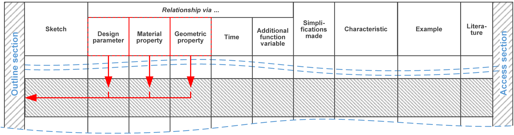
Figure 18. Structuring of the effect catalog via design parameters (material and geometric properties) [translated from Vorwerk-Handing Reference Vorwerk-Handing2021].
4.2.2. Access section of the effect catalog
The aim of the access section of the effect catalog is to enable a preselection of potentially usable physical effects by the user. To enable a comparison between requirements and boundary conditions of the respective physical effects and the considered technical system, required properties of the technical system are derived from the effect-specific requirements and boundary conditions. This step is based on the statement from Pahl et al. (Reference Pahl, Beitz, Feldhusen and Grote2007) that the necessary conditions of a technical system for the realization of a physical effect can be described via geometric, material and kinematic properties of the technical system. In order to be able to carry out the desired comparison systematically and automatically, generally valid properties are defined. The starting point for this is the differentiation between geometric, material and kinematic properties of a technical system.
Geometric properties can be categorized in a generally valid way, e.g., according to Pahl et al. (Reference Pahl, Beitz, Feldhusen and Grote2007) into the characteristics type, shape, position, size and number as well as correspondingly associated characteristics. However, since physical effects usually do not depend on a defined geometry, it is not possible to define required geometric properties for physical effects using such an approach. Since every material object has geometric properties, but a description of these cannot be brought into a generally valid relationship with the requirements of physical effects, geometric properties will not be further included in the effect catalog. However, information about geometric properties of the technical system offers potentials, which can be used in addition to the presented approaches. Particularly against the background of primary function fulfilment by function-relevant design parameters as well as installation space restrictions, the geometric properties of the initial system must be considered individually.
In order to enable a systematic preselection of potentially usable physical effects, material and kinematic properties are considered. On the one hand, material properties can be considered in isolation, related to the respective component of the technical system. Kinematic properties, on the other hand, always require a temporal and/or spatial reference and can thus only be considered at the system level [cf. Sena Reference Sena1972]. Therefore, a differentiation of the required properties into component-dependent and system-dependent properties is made in the effect catalog (cf. Figure 19). It should be noted, however, that the distinction between component- and system-dependent properties depends on the particular point of view.

Figure 19. Structuring of the required properties of a technical system in the access section resulting from effect-specific requirements and boundary conditions [translated from Vorwerk-Handing Reference Vorwerk-Handing2021].
The component-dependent properties are considered in a first step as general material properties and in a second step as application-specific material properties of the respective component. The state of aggregation is used for a general differentiation, cf. Figure 19. Furthermore, the properties listed in the column “relationship via …” in the main content are adopted under the heading “material property”. It must be assessed in each application whether or not the respective material property is available in a usable form.
As system-dependent properties, generally valid kinematic properties of the component in relation to the technical system, are considered in the first step [cf. Pahl et al. Reference Pahl, Beitz, Feldhusen and Grote2007]. According to Pahl et al. (Reference Pahl, Beitz, Feldhusen and Grote2007), the type and form of the movement can be used for this purpose. Further specifications of the mentioned properties are quiescent, translatory or rotatory and uniform, non-uniform or oscillating, cf. Figure 19. In the second step, the function variables listed in the main content in the column “relationship via …” under the heading “additional function variables” are analyzed. In this analysis, it must be assessed in each application whether or not the respective function variable is available in a usable form.
In general, the information listed in the effect catalog in the columns “simplifications made” and “characteristic” can be used to preselect potentially usable physical effects.
The aim of the access section is to provide the opportunity to preselect physical effects based on a comparison between required properties of the component or system under consideration from the effect point of view and existing or producible properties, cf. Figure 20. It is explicitly pointed out that currently existing properties of a component can potentially be changed in order to allow for certain physical effects. In particular, material properties have this potential, provided that the function-relevant properties are not negatively influenced. This can be done by replacing or locally modifying the component in question. Since kinematic properties are usually directly functional-relevant, they typically do not offer this potential. An incompatibility between the properties of a technical system and required properties of a physical effect leads to the exclusion of the respective effect.
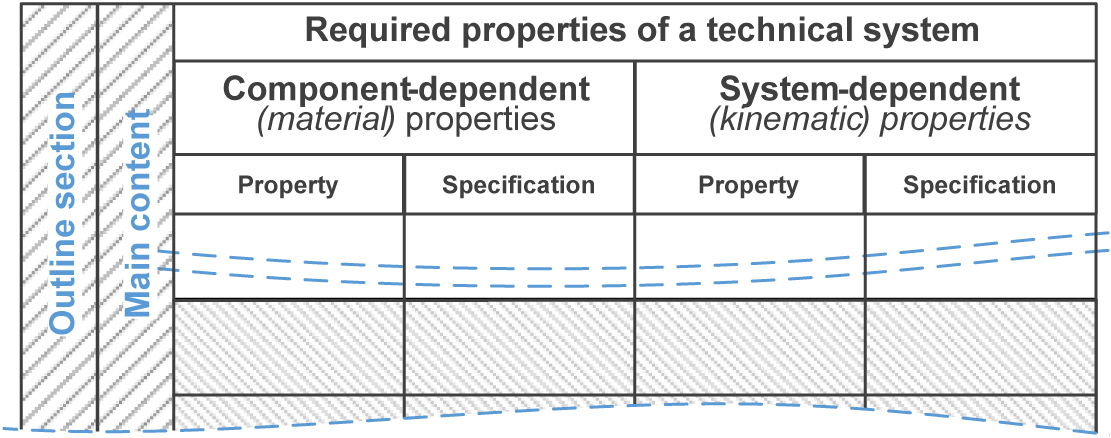
Figure 20. Structure of the effect catalogs’ access section [translated from Vorwerk-Handing Reference Vorwerk-Handing2021].
5. Assessment of the results
The results of Vorwerk-Handing (Reference Vorwerk-Handing2021) were assessed in three consecutive steps using the main objectives from Section 3.2 and additional objectives described in Vorwerk-Handing (Reference Vorwerk-Handing2021):
-
• Application of the developed catalog system using the development of a sensing machine element as an example [Vorwerk-Handing Reference Vorwerk-Handing2021].
-
• Logical verification by means of an argumentation and justification based on a comparison between the defined objectives and the achieved results [Vorwerk-Handing Reference Vorwerk-Handing2021].
-
• Initial validation by an exemplary application of the results in a cooperative industrial project [Harder et al. Reference Harder, Gross, Vorwerk-Handing and Kirchner2021].
With regard to the first two steps, it was found that the developed catalog system and its application enable a systematic establishment of a relationship between a specific state or process variable and potential measurands, taking the (existing) technical system into account. The overarching (positive) impact of the results is yet to be proven based on the situation described in the Section 1. However, Harder et al. (Reference Harder, Gross, Vorwerk-Handing and Kirchner2021) provided an initial proof by applying the results of Vorwerk-Handing (Reference Vorwerk-Handing2021) in the development process of a sensor-integrating plain bearing. In conclusion, Harder et al. (Reference Harder, Gross, Vorwerk-Handing and Kirchner2021) state that “[…] a first application in the industrial project showed itsFootnote 4 advantages. The systematic procedure, with which possible measurands are found for the desired variable of interest, reduces the likelihood of missing a relevant measuring principle. In addition, the approach is applicable without previous experience about metrologically usable relationships or having an expertise with certain machine elements and supports therefore the development of unbiased solutions. […] With these advantages, the presented approach is useful in the methodical development of sensing machine elements and thereby increases the effectiveness of the predictive maintenance of technical systems.”
However, the initial validation also revealed that linking the generated effect chains with the (existing) technical system can be challenging. This is due to the fact that the effect chains typically contain a multitude of different physical effects. In order to be able to make a statement regarding the usability of an effect chain and the associated potential measurand, each of the included physical effects must be analyzed manually with regard to its occurrence in the (existing) technical system. To overcome this limitation, it is reasonable to model the system, its components and their multidomain interactions as well as their properties in a machine-readable way. Therefore, MBSE approaches could prove useful. One possible approach is to use information provided by a SysML model as suggested by Kraus et al. (Reference Kraus, Welzbacher, Schwind, Hahn and Kirchner2023). By doing so, effect chains can be filtered in an automated manner based on the already present – or through minor modifications introducible – geometric, material and kinematic properties of the system and its components. This would leave only effect chains and their associated potential measurands that are already present – or introducible – in the (existing) system. In this way, the identified limitation can be overcome and the usability of the approach can be ensured.
6. Conclusion and outlook
Obtaining reliable information about characteristic process and state variables in existing technical systems is key to their digitalization. However, it is oftentimes not obvious how these variables can be measured in the system, since a measurement can typically be realized in multiple ways – directly as well as indirectly. To solve this problem, the multipole-based effect catalog was developed by Vorwerk-Handing (Reference Vorwerk-Handing2021). Starting from a process or state variable to be determined, the effect catalog and the associated approach allow for a systematic identification of potential measurands in existing technical systems by physical effects.
Starting from existing effect catalog systems as well as their limitations regarding a systematic identification of cause–effect relationships and the fundamentals of multipole-based modeling, a physically and logically justified structure of the multipole-based effect catalog was developed by Vorwerk-Handing (Reference Vorwerk-Handing2021). Since structuring the catalog system strictly according to multipole-based modeling had weaknesses, the initially developed catalog system was pragmatically extended. Furthermore, a consistent differentiation between function variables and function-relevant design parameters was included by Vorwerk-Handing (Reference Vorwerk-Handing2021). The inclusion of design parameters for the consideration of an existing technical system was developed based on multipole-based modeling. Due to its physically and logically justified structuring and the made pragmatic extensions, the developed catalog system is able to map every existing physical effect. This poses a major difference to the software prototype of Helms et al. (Reference Helms, Schultheiss and Shea2013), which could only map 60% of the physical effects included in Koller (Reference Koller1998) and 80.5% of the ones included in Roth (Reference Roth2000).
In summary, a foundation has been created by Vorwerk-Handing (Reference Vorwerk-Handing2021) to systematically include the transformations and changes of a process or state variable in a technical system in the identification process of potential measurands. The results of Harder et al. (Reference Harder, Gross, Vorwerk-Handing and Kirchner2021) firstly demonstrated the potential of the effect catalog in the considered context. However, since the generation of effect chains using the analog multipole-based effect catalog is quite inefficient and prone to error, it was reasonable to digitalize the multipole-based effect catalog. This was carried out by Kraus et al. (Reference Kraus, Matzke, Welzbacher and Kirchner2022, Reference Kraus, Welzbacher, Schwind, Hahn and Kirchner2023), who developed an effect graph based on the multipole-based effect catalog by Vorwerk-Handing (Reference Vorwerk-Handing2021). The effect graph allows for an automated generation of effect chains between a process or state variable to be determined and potential measurands. In addition, Kraus et al. (Reference Kraus, Welzbacher, Schwind, Hahn and Kirchner2023) extended the approach by Vorwerk-Handing (Reference Vorwerk-Handing2021) by an automated robustness evaluation of the generated effect chains.
Future research is planned, in the context of an automated filtering of generated effect chains, linking a process or state variable to be determined and potential measurands, regarding their occurrence in the (existing) technical system. Therefore, a MBSE-based approach is pursued. Modeling the technical system, its components and their multidomain interactions as well as their properties in SysML, automated filtering of effects that do not occur in the technical system can be enabled. This allows the user to focus on promising effect chains for the realization of a sought-after measuring function.
Acknowledgments
The authors thank the Deutsche Forschungsgemeinschaft (DFG, German Research Foundation), which funded the presented research in the framework of the project “Derivation of analysis- and synthesis-methods to manage uncertainty in the development of mechatronic systems with sensor integrating machine elements”.
Financial support
Funded by the Deutsche Forschungsgemeinschaft (DFG, German Research Foundation) – 426030644. Gefördert durch die Deutsch Forschungsgemeinschaft (DFG) - 426030644.


 Open access