


A psychometric function describes how the probability of some perceptual response varies with the magnitude of a stimulus variable. The term was coined by Urban (1908, pp. 106–107) in analogy to the biometric function describing the probability of dying as a function of age. Urban was reporting studies on perceived heaviness in which observers judged whether a comparison weight was lighter, heavier, or as heavy as a reference weight, much like Fechner (Reference Fechner1860/1966) had done earlier. But, in contrast to Fechner’s treatment of the data for measuring discriminative ability, Urban sought to describe analytically how the probabilities of these judgments vary as a function of the difference between the two weights. These ideas were elaborated later (Urban, Reference Urban1910) to address one of the questions that Fechner (Reference Fechner1860/1966, pp. 67–68) raised for a research program on differential sensitivity, namely, “what change occurs in the ratio of right and wrong cases as a function of the magnitude of the comparison weight”.Footnote 1 Today, psychometric functions are routinely fitted to data collected in analogous studies in different research fields for the stimuli and perceptual dimensions of choice in any sensory modality. Their most easily understandable use is for the functional characterization of sensory processes but psychometric functions are also used as a probe in studies investigating the role of contextual, emotional, or attentional factors in cognition.
Researchers are typically interested in psychometric functions as indicators of some aspect of sensory processing, whether for studying isolated sensory processes or for investigating top–down influences on their operation. Many psychometric functions are monotonic and the usual descriptors are their location (presumably indicative of the detection threshold or the point of subjective equality, according to context) and their slope (presumably indicative of the observer’s ability to discriminate small differences in magnitude). But psychometric functions are only the observable manifestation of an interaction of sensory, decisional, and response processes. Ideally, these three components can be separated out not only to assess their individual influences but, most importantly, to ensure that observed effects on the location or slope of the psychometric function are attributed to the correct component.
From the beginning, data to portray the psychometric function can be collected with a variety of designs now referred to as psychophysical methods. All of them share the defining characteristic of collecting data that express how the prevalence of each possible perceptual response varies with the magnitude of the relevant physical dimension of the stimulus (henceforth, stimulus magnitude) and they differ as to the task by which judgments are elicited which, in turn, makes them differ as to the burden on observers and the length of time needed to collect all the necessary data. For instance, in some cases a single stimulus magnitude is presented per trial for observers to make an absolute judgment; in other cases, two stimulus magnitudes are presented for observers to make a relative judgment, which at least doubles the amount of time required to collect each individual judgment. Over the years, the notion settled in that all psychophysical methods are interchangeable in that all of them provide equally suitable data, on the understanding that properties of the psychometric function determined by the method itself can be easily stripped out. For instance, if a single auditory stimulus like a pure tone is presented with different intensities across trials for observers to report whether or not they heard it, the honest observer will never report hearing a tone whose intensity is below some imperceptible level. If, instead, those stimuli are always paired with a zero-intensity tone for observers to choose in which of the two the tone was perceptible, the observer has a fifty-fifty chance of picking the actually imperceptible tone. Understandably, in the former case the psychometric function ranges from 0 to 1 as intensity increases whereas, in the latter, it ranges from .5 to 1 instead, but both functions should otherwise characterize auditory sensitivity identically.
Over decades of psychophysical research, empirical data have stubbornly concurred in displaying features that question the direct interpretability of psychometric functions as expressions of isolated characteristics of sensory processing. Psychometric functions estimated with different psychophysical methods in within-subject studies consistently display discrepant characteristics and provide distinctly different portraits of sensory processes. Almost invariably, incongruence has been explained away post hoc with the pronouncement that different methods activate different processes, followed by interpretation of the resultant psychometric function without further ado as if it still offered uncontaminated information about whichever processes had been called upon. If every new discrepant result were actually caused by yet another hitherto unknown process, not only would we be confronting a complex multiplicity of indeterminate processes, we would be unable to ascertain whether our empirical data are actually addressing our research questions at all. The underlying reality is probably much simpler, if only we were capable of figuring it out.
This paper reviews an attempt in that direction, in three major parts. First, a presentation of aspects of psychophysical data that question the validity of the conventional framework by which such data are interpreted. Second, a presentation of an alternative framework in which the sensory, decisional, and response components of performance are explicitly modeled to allow separating out their influences, and which accounts for all the data peculiarities with which the conventional framework is inconsistent. Finally, an evidence-based presentation of psychophysical practices that should be avoided and those that are recommendable for interpretability of the psychometric function and its landmark points (e.g., thresholds).
The organization of the paper is as follows. The first section describes main classes of methods used to collect psychophysical data. The next section presents the conventional framework by which such data are interpreted. Then comes a section in which several lines of evidence are presented that question the validity of the conventional framework, all of which call for a more comprehensive alternative. Such an alternative, which we call the indecision model, is presented in the following section, along with a discussion of how it accounts for data that are inconsistent with the conventional framework. Empirical evidence explicitly collected to test the validity of the indecision model is presented next. The following section summarizes all of the above in the form of evidence-based recommendations for advisable practices and also for practices that should be avoided by all means. The paper ends with a summary and a discussion of several issues that were only mentioned in passing in the preceding sections, including the use of methods for direct estimation of thresholds without estimation of the psychometric function itself.
Classes of psychophysical methods
In a broad sense, a psychophysical method is a design comprising a series of trials in each of which an observer provides a perceptual judgment upon presentation of one or more stimuli. Several sources have classified them along dimensions such as the number of stimuli that are presented, the type of judgment that is requested, the number of response categories that are allowed, etc. (e.g., Ehrenstein & Ehrenstein, Reference Ehrenstein, Ehrenstein, Windhorst and Johansson1999; Kingdom & Prins, Reference Kingdom and Prins2010; Macmillan & Creelman, Reference Macmillan and Creelman2005; Pelli & Farell, Reference Pelli, Farell, Bass, van Stryland, Williams and Wolfe1995; Wichmann & Jäkel, Reference Wichmann, Jäkel and Wixted2018). These classifications are not consistent with one another and they are not strictly followed by psychophysicists either. For the purposes of this paper, the crucial dimension for classification is the number of stimulus magnitudes that are presented in each trial, not to be mistaken for the number of identifiable stimuli in it. Also relevant for the purposes of this paper is the response format with which observers report their judgment, defined not just by the number of response categories that observers can use but, more importantly, by which categories those are.
The three classes of methods along the dimension of number of stimulus magnitudes are the single-, dual-, and multiple-presentation methods. For reference, consider the visual task of judging the relative location of a short vertical bar placed somewhere along the length of a horizontal line, a bisection task often used to investigate visual space perception and its anomalies (e.g., Olk & Harvey, Reference Olk and Harvey2002; Olk, Wee, & Kingstone, Reference Olk, Wee and Kingstone2004). A single-presentation method displays in each trial the vertical bar at some location (Figure 1a); a dual-presentation method displays two instances of the configuration with the vertical bar generally at a different location in each one (Figure 1b); and a multiple-presentation method simply adds more presentations in a trial (Figure 1c). The single-presentation method was referred to by the early psychophysicists as the method of absolute judgment (e.g., Wever & Zener, Reference Wever and Zener1928) or the method of single stimuli (e.g., Volkmann, Reference Volkmann1932) to distinguish it from the (dual-presentation) method of relative judgments also referred to as the method of right and wrong cases, the constant method, or the method of constant stimuli (Pfaffmann, Reference Pfaffmann1935; today, the term “constant stimuli” denotes a different characteristic that is compatible with single-, dual-, or multiple-presentation methods). This paper considers only single- and dual-presentation methods (but see the Discussion), because adding more presentations does little else but bring unnecessary complications in the vast majority of cases. As seen later, single- and dual-presentation methods differ as to whether the resultant psychometric function is interpretable.

Figure 1. Schematic Illustration of a Sample Sequence of Events in an Individual Trial under (a) Single-Presentation, (b) Dual-Presentation, and (c) Multiple-Presentation Methods.
Each presentation is short and consecutive presentations are separated by an also short inter-stimulus interval (ISI). Observers report the requested perceptual judgment in the designated response format at the end of the trial.
With all classes of methods, in each trial the observer must make a perceptual judgment and report it, a qualitative dimension referred to as the response format. In a single-presentation method like that in Figure 1a, the observer may be asked to report whether the vertical bar appears to be on the left or on the right of the midpoint of the horizontal line (a binary response format), whether it appears to be on or off the midpoint (a meaningfully different binary format), or whether it appears to be on the left, on the right, or at the midpoint (a ternary format). For other perceptual tasks, stimulus dimensions, or sensory modalities, the response formats for single-presentation methods are essentially the same under appropriate wording, although they are sometimes extended by additionally asking observers to report how confident they are of their judgment (e.g., Peirce & Jastrow, Reference Peirce and Jastrow1885), an aspect that will also be left aside in this paper. In dual- and multiple-presentation methods, observers are not asked to respond to each presentation but to make a comparative judgment. In the example of Figure 1b, the observer could be asked to report in which of the two presentations was the vertical bar closer to the midpoint (a binary response format), to report whether or not it was equally close in both presentations (another meaningfully different binary format), or to report either in which of the presentations was the bar closer to the midpoint or else that they appeared to be equally close in both cases (a ternary format). Multiple-presentation methods allow analogous response formats (i.e., which presentation was more extreme in some respect) but they also permit additional formats like reporting which presentation is different from all the rest or which of the remaining presentations is the first one most similar to. The reason that response formats are another important aspect for the purposes of this paper is that not all of them make the resultant psychometric function interpretable.
The conventional theoretical framework
The psychometric function is useful because its primary determinant is the psychophysical function, which expresses the mapping of some physical continuum onto the corresponding perceptual continuum (e.g., weight onto perceived heaviness or physical position onto perceived position). The psychophysical function could be measured directly with any of the classical psychophysical scaling methods (see, e.g., Kornbrot, Reference Kornbrot2016; Marks & Algom, Reference Marks, Algom and Birnbaum1998; Marks & Gescheider, Reference Marks, Gescheider and Wixted2002), but scaling faces many difficulties because humans do not naturally quantify perceived magnitude on a ratio scale. As Fechner (Reference Fechner1860/1966, p. 47) put it, “the immediate judgment we can make in this context (…) is one of more or less, or one of equality, not one of how many times, which true measurement demands and which it is our purpose to derive”.Footnote 2 The psychometric function is an indirect method to determine the psychophysical function, provided a theoretical link can be established between them.
The link is illustrated here for the sample case of a spatial bisection task under the single-presentation method in Figure 1a. Assume that the psychophysical function μ mapping position x in physical space onto position in perceptual space is the linear function
 $${\rm{\mu }}(x) = a + bx,$$
with any constants a ∈ ℝ and b > 0 and where negative values in physical or perceptual space represent positions on the left of an arbitrary origin set for convenience at the physical or perceptual midpoint of the horizontal line. Thus, a = 0 implies μ(0) = 0 so that the physical midpoint maps onto the perceptual midpoint, whereas with a ≠ 0 the perceptual midpoint lies on the left (a > 0) or on the right (a < 0) of the physical midpoint. Assessing distortions of visual space in opposite directions away from the fixation point requires determining whether or not a = 0, and the psychometric function should indicate it in some way.
The perceived magnitude of a stimulus with physical magnitude x is not the fixed value arising from the psychophysical function but, rather, it is a random variable with mean μ(x) and standard deviation σ(x) so that the psychophysical function only describes how average perceived magnitude varies with physical magnitude. A complete characterization thus requires describing how σ varies with x and what is the form of the distribution of perceived magnitude. Without loss of generality, we will assume that perceived magnitude S is a normal random variable with σ(x) = 1. (For cases in which empirical realism dictates that these assumptions be replaced, see García-Pérez, Reference García-Pérez2014a; García-Pérez & Alcalá-Quintana, Reference García-Pérez and Alcalá-Quintana2012a, Reference García-Pérez and Alcalá-Quintana2015a). Then, at the request to judge whether the location of the vertical bar in a given trial was on the left or on the right of the midpoint, it seems reasonable that the observer will set a decision criterion β at S = 0 (i.e., at the perceptual midpoint; see Figure 2) and respond “left” or “right” according to whether perceived position is negative or positive. Formally, the probability of a “right” response at any given spatial position x is
 $$P\left( {{\rm{''right'';}}\,x} \right) = P\left( {S &gt; {\rm{\beta ;}}\,x} \right) = P\left( {Z &gt; {{{\rm{\beta }} - {\rm{\mu }}\left( x \right)} \over {{\rm{\sigma }}\left( x \right)}}} \right) = 1 - \Phi \left( {{{{\rm{\beta }} - {\rm{\mu }}\left( x \right)} \over {{\rm{\sigma }}\left( x \right)}}} \right),$$
Figure 2. Materialization of the Psychometric Function in Single-Presentation Methods.
Gaussian functions indicate the distribution of perceived position at sample physical positions in the spatial bisection stimulus. The psychophysical function in Eq. 1 is the partly occluded solid line on the surface plane, with b = 0.75 in both panels but a = 0 in (a) and a = 1.5 in (b). If the observer responds “right” when perceived position S is on the right of the perceptual midpoint at S = β with β = 0, the probability of a “right” response at each physical position is given by the shaded area in the corresponding Gaussian distribution. The psychometric function in the back projection plane is depicted as a plot of these probabilities and its 50% point indicates the perceptual midpoint, namely, the physical position that the vertical bar must have for the observer to perceive it at the midpoint. Perceptual and physical midpoints coincide in (a) because a = 0; with the psychophysical function in (b) the perceptual midpoint lies at –a/b = −2, or 2 units to the left of the physical midpoint.
where Z is a unit-normal random variable and Φ is the unit-normal cumulative distribution function. With the preceding assumptions, the psychometric function for “right” responses, Ψright, in a single-presentation bisection task with the left–right response format is simply
 $${\Psi _{{\rm{right}}}}\left( x \right) = \Phi \left( {a + bx} \right).$$
This psychometric function is plotted in the projection planes of Figure 2. Fitting the normal ogive in Eq. 3 to responses collected across repeated trials with the bar placed at each of a number of locations allows estimating a and b, that is, the parameters of the psychophysical function in Eq. 1. The estimated perceptual midpoint is the physical point x at which μ(x) = 0, which is the solution of x = −a/b and is such that Ψright evaluates to .5 at that point (the so-called 50% point on the psychometric function). The same argument sustains interpretation of the 50% point on any psychometric function estimated with a single-presentation method, although some situations may involve nonlinear psychophysical functions, non-normal distributions, or a criterion β placed elsewhere in perceptual space. The general form of the psychometric function is always that of Eq. 2 under the conventional framework, with only a replacement of Φ with the cumulative distribution function that holds in the case under consideration. And one would certainly like to be sure that the 50% point on the psychometric function has this precise interpretation always.
The conventional framework for interpretation of psychometric functions in dual-presentation methods is analogous but the observer’s response is now determined by a comparison of the two perceived magnitudes in each trial. For illustration, consider a visual contrast discrimination task in which the observer reports which of two patterns like those in Figure 3a has a higher contrast. One of the patterns (the standard) has the exact same contrast x s in all trials whereas the contrast x of the other (the test) varies across trials. In this example, standard and test differ on a dimension (spatial frequency) other than the dimension of comparison (luminance contrast). In these circumstances, it is likely that contrast perception is governed by psychophysical functions μs (for the standard) and μt (for the test) that differ from one another (see Figure 3b), rendering normal random variables possibly also with different standard deviations σs and σt. In any case, each trial produces a perceived contrast S s for the standard (drawn from the black distribution in Figure 3b) and a perceived contrast S t for the test (drawn from the applicable red distribution in Figure 3b). It seems reasonable that the observer will respond according to whether the perceived difference D = S t − S s is positive or negative, where D is by our assumptions a normal random variable with mean  ${{\rm{\mu }}_{\rm{t}}}\left( x \right) - {{\rm{\mu }}_{\rm{s}}}\left( {{x_{\rm{s}}}} \right)$ and variance
  ${\rm{\sigma }}_{\rm{D}}^2\left( x \right) = {\rm{\sigma }}_{\rm{t}}^2\left( x \right) + {\rm{\sigma }}_{\rm{s}}^2\left( {{x_{\rm{s}}}} \right)$. Modeling the decision process requires consideration of the distribution of D at different test contrasts (see Figure 3c), with a decision criterion at the null difference (i.e., β = 0) so that the observer responds “test higher” when D > 0 and “test lower” when D < 0.Footnote 3 Then, the probability of a “test higher” response at a given test contrast x is
 $$P\left( {{\rm{''higher'';}}\,x} \right) = P\left( {D &gt; {\rm{\beta ;}}\,x} \right) = P\left( {Z &gt; {{{\rm{\beta }} - \left( {{{\rm{\mu }}_{\rm{t}}}\left( x \right) - {{\rm{\mu }}_{\rm{s}}}\left( {{x_{\rm{s}}}} \right)} \right)} \over {{{\rm{\sigma }}_{\rm{D}}}\left( x \right)}}} \right) = \Phi \left( {{{{{\rm{\mu }}_{\rm{t}}}\left( x \right) - {{\rm{\mu }}_{\rm{s}}}\left( {{x_{\rm{s}}}} \right) - {\rm{\beta }}} \over {{{\rm{\sigma }}_{\rm{D}}}\left( x \right)}}} \right).$$
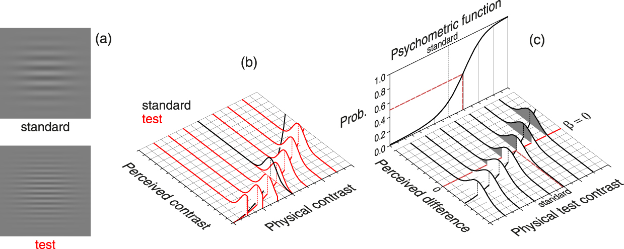
Figure 3. Materialization of the Psychometric Function in Dual-Presentation Methods.
(a) Stimuli for a contrast discrimination task with standard and test that differ in spatial frequency. (b) Psychophysical functions for standard (black curve on the plane) and test (red curve on the plane) reflect differences in the mapping of physical onto perceived contrast at different spatial frequencies. Psychophysical functions are given by  ${{\rm{\mu }}_i}\left( x \right) = {a_i}{x^{{b_i}}}$, with i ∈ {s, t} for standard (s) and test (t), a s = 0.7, a t = 0.5, and b s = b t = 1.6. Unit-variance Gaussians depict the distribution of perceived contrast for the standard (black distribution, which is the same in all trials) and for the test (red distributions, which varies across trials). (c) Distributions of perceived difference as a function of the physical contrast of the test. If the observer responds “test higher” when the perceived difference D is positive (i.e., β = 0), the probability of a “test higher” response at each test contrast is given by the shaded area in the corresponding distribution. The psychometric function is depicted as a plot of these probabilities and its 50% point indicates the point of subjective equality (PSE), namely, the physical contrast that the test must have for the observer to perceive it as having the same contrast as the standard.
With β = 0, this psychometric function has its 50% point at  $x = {\rm{\mu }}_{\rm{t}}^{ - 1}\left( {{{\rm{\mu }}_{\rm{s}}}\left( {{x_{\rm{s}}}} \right)} \right)$, that is, at the test contrast whose perceived contrast (via the psychophysical function μt) equals the perceived contrast of the standard (via the function μs). In other words, the 50% point on the psychometric function indicates the point of subjective equality (PSE) and, thus, reveals differences in the psychophysical functions μs and μt whenever the PSE is found to lie away from the standard magnitude x s. Similarly, the slope of the psychometric function is indicative of the observer’s capability to discriminate small differences in contrast between test and standard, providing an estimate of the difference limen (DL) defined as the difference between the PSE and the point at which the psychometric function evaluates to, say, .75. Many empirical studies use dual-presentation methods to estimate PSEs or DLs and, again, one needs assurance that the location and slope of the psychometric function always allow an interpretation in terms of PSEs and DLs beyond the fact that a psychometric function of this type will always have 50% and 75% points somewhere.
Evidence questioning the validity of the conventional framework
The preceding section described the conventional framework that justifies the interpretation of psychometric functions estimated with single- or dual-presentation methods, which in turn allows estimating the psychophysical function from the psychometric function and justifies extracting from the psychometric function the characteristics that are relevant to the research goals (perceptual midpoints, PSEs, DLs, etc.). Yet, a vast amount of empirical data collected over decades of research with single- and dual-presentation methods questions the validity of such a framework and justification. Specifically, data from numerous studies display features that are logically incompatible with the conventional framework. This section summarizes them, first for data collected with dual-presentation methods because they were developed and used more thoroughly in early psychophysics and also because this is where the problems were immediately obvious from day one. Nagging peculiarities of data collected with single-presentation methods will be presented afterwards.
Undecided cases in dual-presentation methods
Fechner (Reference Fechner1860/1966, p. 77) reported that the experiments he started in 1855 were designed to be a more exact check of Weber’s law but he soon realized that a thorough investigation of the implications of procedural details should be undertaken first. One of his concerns was whether observers should be forced to respond in each trial that the second weight was either perceptually heavier or lighter than the first or, instead, they should be allowed to express indecision and report the two weights to be perceptually equally heavy whenever needed. He sentenced that “in the beginning I always used the first procedure, but later I discarded all experiments done in that way and used the second course exclusively, having become convinced of its much greater advantages” (p. 78).
The undecided response had been allowed earlier by Hegelmaier (1852; translated into English by Laming & Laming, Reference Laming and Laming1992) in a study on the perceived length of lines, a work that Fechner credited. Despite some opposition (see Fernberger, Reference Fernberger1930), the undecided response continued to be allowed until signal detection theory took over and denied undecided cases entirely, although there were attempts to reinstate it that did not seem to stick (e.g., Greenberg, Reference Greenberg1965; Olson & Ogilvie, Reference Olson and Ogilvie1972; Treisman & Watts, Reference Treisman and Watts1966; Vickers, Reference Vickers, Rabbitt and Dornic1975, Reference Vickers1979; Watson, Kellogg, Kawanishi, & Lucas, Reference Watson, Kellogg, Kawanishi and Lucas1973). The influence of signal detection theory is perhaps the reason that the conventional framework invariably assumes a decision rule by which observers are never undecided and always respond according to whether the decision variable is above or below some criterion β. Ironically, and despite interpreting the data as if observers could never be undecided, undecided cases are explicitly acknowledged in practice and observers are instructed to guess in such cases. Undoubtedly, undecided cases are impossible under the conventional framework and they ask for an amendment that can capture them adequately to allow proper inferences from observed data. In fact, the consequences of ignoring them are serious, as will be seen below. It is worth saying in anticipation that neither the admonition to guess when undecided nor Fechner’s strategy of counting undecided responses as half right and half wrong are advisable: They both distort the psychometric function in ways that it no longer expresses the true characteristics of the psychophysical function and, thus, neither the location nor the slope of the psychometric function reflect the underlying reality that researchers aim at unveiling.
A closely related issue that calls for an analogous amendment is that many studies use dual-presentation methods under the same–different task (see Macmillan & Creelman, Reference Macmillan and Creelman2005, pp. 214–228; see also Christensen & Brockhoff, Reference Christensen and Brockhoff2009), sometimes referred to as the equality task to distinguish it from the previously discussed comparative task where observers report which stimulus is stronger in some respect. The equality task also implies a binary response but now observers indicate only whether the two stimuli appear to be equal or different along the dimension of comparison. Leaving aside the sterile discussion as to whether responding “same” in the equality task is tantamount to being undecided in the comparative task, it is nevertheless clear that the same–different task is incompatible with the conventional framework: With a single boundary (at β = 0 as in Figure 3c or elsewhere), observers should invariably respond “different” in all trials. It certainly does not seem sensible to amend the decision space only for the same–different task, because it would then imply that whether an observer can or cannot judge equality depends on the question asked at the end of the trial, which can indeed be withheld so the observer gets to know it only after the stimuli are extinguished (see the control experiment reported by Schneider & Komlos, Reference Schneider and Komlos2008). The conventional framework thus also needs an amendment to accommodate the empirical fact that observers can perform the same–different task if so requested, and this must be done in a way that is consistent with the fact that observers often guess in the comparative task.
Order or position effects in dual-presentation methods. Part I: The constant error
Presentation of two magnitudes cannot occur co-spatially and simultaneously. Then, standard and test have to be presented in some temporal order or in some spatial arrangement in each trial. Fechner (Reference Fechner1860/1966, pp. 75–77) reported that the temporal order in which the two weights were lifted greatly affected the results in a way that the ratio of right to wrong cases turned out quite different and beyond what could be expected by chance even with long series of trials. This was regarded as evidence of a so-called constant error, which is puzzling because it implies that standard and test stimuli of the exact same magnitude and also identical in all other respects are systematically perceived to be different according to the order or position in which they are presented. Fechner also reported that constant errors varied in size across sessions for the same observer and that the cause of their “totally unexpected general occurrence” (p. 76) was unclear, but he found solace by accepting them as a constituent part of psychophysical measurements. He also devised a method to average out their influence so that unique estimates of differential sensitivity could still be obtained. Unbeknownst to Fechner, such unique estimates are essentially flawed, as will be seen below.
Fechner was mainly interested in investigating Weber’s law, which requires that standard and test stimuli differ exclusively in their magnitude along the dimension of comparison. The ubiquitous presence of constant errors becomes an obstacle to this endeavor because it implies that standard and test stimuli differ also on something else by an unknown mechanism related to procedural factors. Measures of differential sensitivity reflecting how much heavier the test must be for observers to notice a difference in heaviness cannot be obtained when the perceived heaviness of the standard differs due to such procedural factors. Although the notion of a psychometric function was not available to Fechner, in present-day terms his studies sought to measure the DL as defined earlier. But this, of course, requires that a test stimulus with the exact same weight as the standard stimulus is actually perceived to be as heavy as the standard, a pre-condition that the presence of constant errors violates.
Figure 4 illustrates what the psychometric function should be like under the conventional framework when test and standard are identical except in magnitude along the dimension of comparison (visual luminance contrast in this case), which in comparison to Figure 3 only differs in that test and standard stimuli have the same spatial frequency and, thus, μt = μs. The PSE is predicted to be at the standard contrast and the DL as defined earlier can be computed from the slope of the function. But constant errors defy this framework, because they imply a lateral shift of the psychometric function such that the 50% point is no longer at the standard and the 75% point is similarly shifted. Despite the shift, differential sensitivity might still be assessed if it is computed relative to the (shifted) location of the 50% point rather than relative to the actual location of the standard. If the unknown mechanism only shifts the psychometric function laterally without affecting its slope, constant errors will not be a problem provided that the necessary precautions are taken to compute sensitivity measures adequately. We will show later that this is not the case, but something must still be missing in the conventional framework when it cannot account for the occurrence of constant errors.

Figure 4. Psychometric Function Arising from the Conventional Framework when Test and Standard Stimuli Differ only along the Dimension of Comparison so that μt = μs.
The 50% point is then at the standard level and, thus, at the perceptual PSE. Layout and graphical conventions as in Figure 3.
Constant errors have been around since Fechner but their cause was not investigated by the early psychophysicists. Interest soon focused on methodological research to establish optimal conditions for preparation and administration of stimuli and for the collection of data with the ternary response format. In this context, figuring out how to eliminate constant errors was not as much a priority as was keeping their influence constant. Thus, for the sake of experimental control, Urban (Reference Urban1908) always used sequential presentations in which the standard weight was lifted before the test weight in each trial (a strategy that was later referred to as the reminder paradigm; see Macmillan & Creelman, Reference Macmillan and Creelman2005, pp. 180–182). The data that Urban reported in tabulated or graphical form invariably reflected constant errors in the form of psychometric functions shifted laterally, suggesting that the PSE was not at the standard magnitude but somewhat below it. Fernberger (Reference Fernberger1913, Reference Fernberger1914a, Reference Fernberger1914b, Reference Fernberger1916, Reference Fernberger1920, Reference Fernberger1921) also used the reminder paradigm in analogous studies aimed at perfecting the experimental procedure and investigating additional issues so that, again, the constant error was regarded as an extraneous factor simply kept constant in the interest of experimental control.
We are not aware of any early study in which both orders of presentation (i.e., standard first and standard second) had been used in separate series in a within-subjects design to ascertain how psychometric functions under the ternary response format used at that time differ across presentation orders. Some studies were conducted along these lines, but with undecided responses already transformed into half right and half wrong (e.g., Woodrow, Reference Woodrow1935; Woodrow & Stott, Reference Woodrow and Stott1936). Some research conducted during the second half of the 20th century used the binary format asking observers to guess when undecided, but these studies only measured constant errors at isolated pairs of magnitudes with no possibility of looking at psychometric functions (e.g., Allan, Reference Allan1977; Jamieson & Petrusic, Reference Jamieson and Petrusic1975). Ross and Gregory (Reference Ross and Gregory1964) appeared to be the first to conduct a study of constant errors under each of the possible presentation orders, but they also forced observers to guess when undecided. In other studies, psychometric functions were also measured but only with the reminder paradigm and using the binary response format with guesses (e.g., Levison & Restle, Reference Levison and Restle1968).
It should be noted that the PSE empirically determined from the 50% point on an observed psychometric function is only a misnomer in the presence of constant errors. In fact, when standard and test are identical in all respects, a PSE declared to be away from the standard would literally mean that a stimulus has to be different from itself for an observer to perceive them both as equal. This nagging incongruence was handled in early psychophysics by defining the constant error as the difference between the observed PSE and the standard, on the implicit assumption that the true PSE was indeed located at the standard and that the observed deviation was only disposable error of an unknown origin. Unfortunately, there is a large set of situations in which one cannot reasonably assume that the true PSE is at the standard, as in studies aimed at investigating whether and by how much the psychophysical function for some stimulus dimension varies across extra dimensions, where one has reasons to believe that μt ≠ μs as illustrated in Figure 3. All studies on perceptual illusions also fall in this class (e.g., whether and by how much the perceived length of a line varies when it terminates in arrowheads vs. arrow tails in the Müller–Lyer figure, or whether and by how much the perceived luminance of a uniform gray field varies with the luminance of the background it is embedded in), and other types of studies also fall in this category (e.g., whether and by how much does perceived contrast vary with spatial frequency, or whether and by how much the perceived duration of an empty interval differs from that of a filled interval). In such cases, constant errors make it impossible to determine whether a 50% point found to be away from the standard reflects different psychophysical functions for test and standard. Then, an amendment to the conventional framework seems necessary to incorporate a mechanism that produces constant errors so as to be able to extract the characteristics of the underlying psychophysical functions and, thus, to establish with certainty whether a 50% point that is found to be away from the standard magnitude is only disposable error or a true indication that test and standard stimuli are perceived differently.
Order or position effects in dual-presentation methods. Part II: Interval bias
Although constant errors continued to be a topic of research (for recent papers and references to earlier studies, see Hellström & Rammsayer, Reference Hellström and Rammsayer2015; Patching, Englund, & Hellström, Reference Patching, Englund and Hellström2012), they have been ignored in research estimating psychometric functions with dual-presentation methods. It is not easy to trace back the time at which (and to dig out the reasons why) this happened, but around the 1980’s it became customary to intersperse at random trials presenting the standard first or second and to bin together all the responses given at each test magnitude irrespective of presentation order to fit a single psychometric function to the aggregate. The ternary response format had also long been abandoned and observers were routinely forced to guess when undecided. The notion of “constant error” then resurfaced under the name “interval bias” to refer to differences in the observed proportion of correct responses contingent on the order of presentation of test and standard, although the term had been used earlier by Green and Swets (1966, pp. 408–411) in a context not involving estimation of psychometric functions, and only at that point within their entire book.
Nachmias (Reference Nachmias2006) seems to have been the first to fit and plot separate psychometric functions for the subsets of trials in which the test was first or second, although he appeared to have used for this purpose aggregated data across all available observers and experimental conditions. His results revealed that interval bias (constant error) was also present when trials with both orders of presentation were randomly interwoven in a session and, thus, not only when separate sessions were conducted for each order as Ross and Gregory (Reference Ross and Gregory1964) had done earlier. In line with Hellström (Reference Hellström1977), this suggested that the constant error is perceptual in nature and not due to a response bias developed over the course of a session with trials of the same type. Again, this result questions the validity of the conventional framework, which assumes that μt = μs when test and standard are identical except along the dimension of comparison and invariant with presentation order.Footnote 4 An interval bias of perceptual origin would imply that the psychophysical functions differ when the stimulus (test or standard) is presented first or second, even when such stimuli are identical. There are good reasons to think that this might indeed occur with intensive magnitudes due to desensitization or analogous influences from the first presentation on the second (see Alcalá-Quintana & García-Pérez, Reference Alcalá-Quintana and García-Pérez2011), but this is instead impossible with the extensive magnitudes for which interval bias and constant errors have been described more often.
Interval bias has been found in data sets that were originally treated conventionally (i.e., by aggregating responses across presentation orders) but for which the order of presentation in each trial had been recorded and a re-analysis was possible (García-Pérez & Alcalá-Quintana, Reference García-Pérez and Alcalá-Quintana2011a). Interval bias was also found in new studies intentionally conducted to investigate it (e.g., Alcalá-Quintana & García-Pérez, 2011; Bausenhart, Dyjas, & Ulrich, Reference Bausenhart, Dyjas and Ulrich2015; Bruno, Ayhan, & Johnston, Reference Bruno, Ayhan and Johnston2012; Cai & Eagleman, Reference Cai and Eagleman2015; Dyjas, Bausenhart, & Ulrich, Reference Dyjas, Bausenhart and Ulrich2012; Dyjas & Ulrich, Reference Dyjas and Ulrich2014; Ellinghaus, Ulrich, & Bausenhart, Reference Ellinghaus, Ulrich and Bausenhart2018; García-Pérez & Alcalá-Quintana, 2010a; Ulrich & Vorberg, Reference Ulrich and Vorberg2009). Many of these studies have documented order effects in two different forms that Ulrich and Vorberg called “Type A” and “Type B”. The former is the lateral shift that we have described thus far; the latter is a difference in the slope of the psychometric functions for each presentation order, which can be observed with or without lateral shifts. Whichever its origin may be, an amendment to the conventional framework is necessary to account for the empirical fact that psychometric functions vary with the order or position of presentation of test and standard.
Effects of response format in single-presentation methods
Presentation of a single magnitude per trial certainly removes any potential complication arising from order effects, but there are still aspects of single-presentation data that are incompatible with the conventional framework. One feature on which available single-presentation methods differ from one another is the response format with which judgments are collected. And one form in which the conventional framework fails here is by being unable to account for differences in the psychometric functions or their characteristics across response formats, which should imply the same psychophysical functions because the operation of sensory systems cannot be retroactively affected by how observers report their judgments. We will only discuss two of the various lines of evidence in this direction.
One of them arises in the context of research on perception of simultaneity. These studies rest on earlier procedures developed to determine the smallest inter-stimulus temporal gap that can be experienced (see James, Reference James1886) and they were originally designed by Lyon and Eno (Reference Lyon and Eno1914) to investigate the transmission speed of neural signals with the method of constant stimuli. Trials consisted of the administration of punctate tactual or electrical stimuli on different parts of the arm with a variety of temporal delays. The rationale is that transmission speed can be estimated by measuring how much earlier stimulation at a distal location must be administered for an observer to perceive it synchronous with stimulation at a proximal location. Two stimuli are obviously used here but a single value of the dimension under investigation (namely, temporal delay) is presented in each trial, so this is one of the single-presentation methods in which two identifiable stimuli are required to administer a single magnitude along a dimension unrelated to any of the physical characteristics of the stimuli themselves. Contrary to the spirit of their time, Lyon and Eno asked observers to report which stimulus had been felt first, disallowing “synchronous” responses and forcing observers to guess. The exact same strategy is still used today under the name temporal-order judgment (TOJ) task, but variants thereof include the binary synchrony judgment (SJ2) task in which observers simply report whether or not the presentations were perceptually synchronous, and the ternary synchrony judgment (SJ3) task which is a TOJ task with allowance to report synchrony (Ulrich, Reference Ulrich1987). Usually, the purpose of these studies is to determine the point of subjective simultaneity (PSS), defined as the delay with which one of the stimulus must be presented for observers to perceive synchronicity. One of the most puzzlingly replicated outcomes of this research is that PSS estimates meaningfully vary across tasks within observers (see, e.g., van Eijk, Kohlrausch, Juola, & van de Par, Reference van Eijk, Kohlrausch, Juola and van de Par2008), with differences such that the delay at which “synchronous” responses are maximally prevalent in SJ2 or SJ3 tasks is also one of those at which asynchronous responses of one or the other type prevail in the TOJ task. The typical ad hoc argument to explain away these contradictory outcomes is to assume that each task calls for different cognitive processes, which goes hand in hand with the far-fetched assumption that the psychophysical function mapping physical asynchrony onto perceived asynchrony varies with the response format.
The second line of evidence arises in research on perception of duration and, specifically, on the ability to bisect a temporal interval, which is generally investigated with either of two alternative single-presentation methods. In the temporal bisection task (Gibbon, Reference Gibbon1981), observers report during an experimental phase whether intervals of variable duration are each closer in length to a “short” or to a “long” interval repeatedly presented earlier during a training phase; in the temporal generalization task (Church & Gibbon, Reference Church and Gibbon1982), observers report during the experimental phase whether or not the temporal duration of each of a set of individually presented intervals is the same as that of a “sample” interval repeatedly presented during the training phase. Not unexpectedly in the context of this discussion, the temporal bisection point has been found to vary meaningfully with the variant used to collect data (e.g., Gil & Droit-Volet, Reference Gil and Droit-Volet2011), which again seems to suggest that the psychophysical function mapping chronometric duration onto perceived duration varies with the response format.
Note that the various response formats in each of these research areas (TOJ vs. SJ2 or SJ3 in perception of simultaneity and bisection vs. generalization in perception of duration) resemble those discussed earlier for dual-presentation methods (comparative vs. equality). Just as a single-boundary decision space could never give rise to “same” responses in a dual-presentation method, never would it give rise to “synchronous” or “same” responses in the single-presentation methods just discussed. It may well be that these apparent failures of the conventional framework are another manifestation of the consequences of forcing (in TOJ or bisection tasks) or not forcing (in SJ2, SJ3, or generalization tasks) observers to give responses that do not reflect their actual judgment of synchrony in onset or equality in duration. Then, this is another area where an alternative framework that reconciles these conflicting results is needed.
Effects of response strategy in single-presentation methods
Another line of evidence against the conventional framework for single-presentation methods comes from studies in which data are collected under different conditions or instructions aimed at manipulating the observers’ decisional or response strategies. Admittedly, the effect of some of these manipulations are still compatible with the conventional framework as long as they can be interpreted as altering the location of criterion β (see, e.g., Allan, Reference Allan2002; Ellis, Klaus, & Mast, Reference Ellis, Klaus and Mast2017; Raslear, Reference Raslear1985; Wearden & Grindrod, Reference Wearden and Grindrod2003). Even with such allowance, this reveals an inescapable problem that will be discussed later, namely, that single-presentation methods confound sensory and decisional components of performance (see García-Pérez & Alcalá-Quintana, Reference García-Pérez and Alcalá-Quintana2013) and leave researchers unable to figure out if they are observing a relevant result indicative of the characteristics of sensory processing (a feature of the psychophysical function) or an outcome reflecting only the effect of non-sensory factors (an influence of the location of the response criterion). Yet, the interest in investigating some instructional manipulations and the fact that they happen to produce effects are inherently incongruent with the conventional framework, which ignores all of these influences entirely. For instance, Capstick (2012, exp. 2) reported the results of a within-subjects study that used two variants of the single-presentation TOJ task respectively differing in that observers were asked to always give one or the other allowed responses when uncertain. The 50% point on the psychometric function for each variant of the TOJ task shifted in opposite directions away from physical simultaneity, which is inexplicable under the conventional framework with single decision boundary. In line with this result, Morgan Dillenburger, Raphael, and Solomon (2012) reported the same effect on the psychometric function in a spatial bisection task under the binary left–right format: It shifted laterally according to instructions as to how to respond when uncertain so that the 50% point on the psychometric function came out on the far left of the physical midpoint in one case and on the far right in the other. Which of these two, if any, is the PSS or the perceptual midpoint? The dissonance is further apparent because observers can never be uncertain under the conventional decision space (see Figure 2) and, hence, instructions as to what to do in those (inexisting) cases should be inconsequential. Of course, the fact that such instructions produce effects on the location of the psychometric function implies again that something is missing in the conventional framework, further stressing that the observed location of a psychometric function is not necessarily indicative of the characteristics of the psychophysical function mapping a physical continuum maps onto its perceptual counterpart.
An alternative framework: The indecision model
This section describes an amendment to the conventional framework that accounts for all of the anomalies of single- and dual-presentation data just discussed. The alternative framework, which we call indecision model, keeps the assumptions about the role of the psychophysical function(s) intact but it changes the assumption about how the decision space is partitioned into exhaustive and mutually exclusive regions associated with perceptual judgments, and it also adds assumptions about how these judgments are expressed under the designated response format. The indecision model is thus a process model explicitly representing the sensory, decisional, and response components of performance via distinct parameters that can be estimated to separate out their influences. In other words, the model does not simply add shape parameters to psychometric functions of a convenient but arbitrary functional form; instead it generates the psychometric function from functional descriptions of the operation of sensory, decisional, and response processes. A formal presentation of the indecision model for single- and dual-presentation methods in a diversity of contexts has been given elsewhere (see García-Pérez, Reference García-Pérez2014a; García-Pérez & Alcalá-Quintana, Reference García-Pérez and Alcalá-Quintana2011a, Reference García-Pérez and Alcalá-Quintana2012a, Reference García-Pérez and Alcalá-Quintana2013, Reference García-Pérez and Alcalá-Quintana2015a, Reference García-Pérez and Alcalá-Quintana2015b, Reference García-Pérez and Alcalá-Quintana2017, Reference García-Pérez, Alcalá-Quintana, Vatakis, Balcı, Di Luca and Correa2018; García-Pérez & Peli, Reference García-Pérez and Peli2014, Reference García-Pérez and Peli2015, Reference García-Pérez and Peli2019; see also Self, Mookhoek, Tjalma, & Roelfsema, Reference Self, Mookhoek, Tjalma and Roelfsema2015; Tünnermann & Scharlau, Reference Tünnermann and Scharlau2018) and here we will opt for an informal presentation in the context of sample cases considered earlier.
The (not really novel; see below) main aspect of the indecision model is its positing that the number of partitions in perceptual space (i.e., the number of distinct perceptual judgments that an observer can make) may and generally will be larger than the number of permitted response categories. Hence the need of rules by which judgments are expressed as responses (e.g., how judgments of equality are reported when only “weaker” or “stronger” responses are permitted). This section presents theoretical arguments and empirical data demonstrating how the indecision model accounts for the anomalies described in the preceding section, first for single-presentation methods and then for dual-presentation methods. It should be noted that this is not the only way in which the conventional framework can be amended to reconcile theory with data, but it is certainly the most comprehensive. Other alternatives will be briefly presented and commented on in the Discussion.
The indecision model in single-presentation methods
The simple decision space of the conventional framework in the sample application of the single-presentation method in Figure 2 might actually involve as many regions along the dimension of perceived position as positions an observer is capable of discerning (e.g., slightly on the right, far on the right, etc.). Qualitative and ill-defined categories of this type were indeed used in the method of absolute judgment by the early psychophysicists. For instance, Fernberger (Reference Fernberger1931) had observers classify each individually lifted weight into the three categories of light, intermediate, or heavy. Analogously, in a study on taste, Pfaffmann (Reference Pfaffmann1935) asked observers to rate the intensity of each tastant on a six-point scale. A potential gradation of the perceptual continuum with multiple boundaries is accepted even by signal detection theorists, as it is the basis for classification, identification, and rating designs (Green & Swets, Reference Green and Swets1966, pp. 40–43; Macmillan, Kaplan, & Creelman, Reference Macmillan, Kaplan and Creelman1977; Wickelgren, Reference Wickelgren1968). A single-presentation method with multiple ordered response categories that capitalize on this gradation is a quantized psychophysical scaling method without the burden of arbitrary and unnatural numerical scales (Galanter & Messick, Reference Galanter and Messick1961). Arguably, these regions might be the basis by which observers express confidence when so requested, although we will not discuss this here (but see Clark, Yi, Galvan-Garza, Bermúdez Rey, & Merfeld, Reference Clark, Yi, Galvan-Garza, Bermúdez Rey and Merfeld2017; Lim, Wang, & Merfeld, Reference Lim, Wang and Merfeld2017; Yi & Merfeld, Reference Yi and Merfeld2016).
Without loss of generality, we will restrict ourselves here to cases in which the partition can be anchored relative to a well-defined internal reference such as the perceptual midpoint, the subjective vertical, subjective synchrony, perceptual straight ahead, etc. A defining assumption of the indecision model is that the smallest possible number of partitions after any necessary aggregation is three and that the central region stretches around the location of the internal reference (the null value in perceptual space in all of the sample cases just mentioned) but not necessarily centered with it, as seen in Figure 5. This minimum number of three regions does not deny subdivisions that might manifest if the response format asked observers to use them (e.g., by expanding the response set to include, say, slightly on the right, far on the right, etc.). What the indecision model posits is that there are three qualitatively different regions, even if the response format only asks for a binary response. In other words, the boundaries δ1 and δ2 (with δ1 < δ2) of the central region in Figure 5 will not come together by simply forcing observers to give a binary left–right response. Or, yet in other words, judgments of “center” (under any suitable designation) are qualitatively different from, and impossible to collapse with, judgments of “left” or “right”, whereas judgments of degrees of “left” (or “right”) to several discernible extents can and will be collapsed into a qualitative judgment of “left” (or “right”) if no gradation is required by the response format. This central region can be regarded as the interval of perceptual uncertainty to stress that it is defined in perceptual space and, thus, not to be confused with the interval of uncertainty defined by Fechner (Reference Fechner1860/1966, p. 63) and further elaborated by Urban (1908, Ch. V) to represent the range of stimulus magnitudes where undecided responses prevail.

Figure 5. Alternative Framework of the Indecision Model in the Single-Presentation Example of Figure 2 with a Partition of Perceptual Space into Three Regions Demarcated by Boundaries δ1 and δ2 that Can Be Symmetrically Placed with Respect to the Perceptual Midpoint (a) or Displaced (b).
In either case, when the spatial bisection task is administered with the response options “left”, “right”, and “center”, the psychometric functions come out as shown in the back projection planes. Although the same psychophysical function mapping the physical midpoint onto the perceptual midpoint is used in both cases, the peak of the psychometric function for “center” responses does not occur at the physical midpoint in (b) due to the displacement of the region for “center” judgments.
With allowance for “center” responses so that there is a one-to-one mapping between (qualitatively different) judgments and responses, the psychometric functions come out as illustrated in the back projection planes in Figure 5 and are given by
 $$P\left( {{\rm{''left'';}}\,x} \right) = P\left( {S &lt; {{\rm{\delta }}_1}{\rm{;}}\,x} \right) = P\left( {Z &lt; {{{{\rm{\delta }}_1} - {\rm{\mu }}\left( x \right)} \over {{\rm{\sigma }}\left( x \right)}}} \right) = \Phi \left( {{{{{\rm{\delta }}_1} - {\rm{\mu }}\left( x \right)} \over {{\rm{\sigma }}\left( x \right)}}} \right)$$,
 $$P\left( {{\rm{''right'';}}\,x} \right) = P\left( {S &gt; {{\rm{\delta }}_2}{\rm{;}}\,x} \right) = P\left( {Z &gt; {{{{\rm{\delta }}_2} - {\rm{\mu }}\left( x \right)} \over {{\rm{\sigma }}\left( x \right)}}} \right) = \Phi \left( {{{{\rm{\mu }}\left( x \right) - {{\rm{\delta }}_2}} \over {{\rm{\sigma }}\left( x \right)}}} \right)$$,
 $$P\left( {{\rm{''center'';}}\,x} \right) = P\left( {{{\rm{\delta }}_1} &lt; S &lt; {{\rm{\delta }}_2}{\rm{;}}\,x} \right) = \Phi \left( {{{{{\rm{\delta }}_2} - {\rm{\mu }}\left( x \right)} \over {{\rm{\sigma }}\left( x \right)}}} \right) - \Phi \left( {{{{{\rm{\delta }}_1} - {\rm{\mu }}\left( x \right)} \over {{\rm{\sigma }}\left( x \right)}}} \right)$$,
with the probabilities at each position x indicated by the areas colored in red, gray, and blue, respectively, under the Gaussian distributions of perceived position in Figure 5. In Figure 5a, the peak of the psychometric function for center responses occurs at the physical midpoint, reflecting that the psychophysical function in this example is given by Eq. 1 with a = 0. Then, the location of the psychometric functions reveals no distortion of perceptual space. Yet, this is only because the boundaries δ1 and δ2 are also symmetrically placed with respect to the perceptual midpoint (i.e., δ1 = −δ2). If these boundaries were displaced (i.e., δ1 ≠ −δ2; see Figure 5b), the psychometric functions also get displaced, producing the appearance of a perceptual distortion of space despite the fact that the underlying psychophysical function with a = 0 still maps the physical midpoint onto the perceptual midpoint in this example. In general, the empirical finding of displaced psychometric functions is not necessarily indicative of a true perceptual distortion. In the case of Figure 5b, the displacement is only caused by what we call decisional bias: An off-center location of the interval of perceptual uncertainty by which the amount of evidence needed for a “left” judgment differs from that needed for a “right” judgment. (We will comment on empirical evidence to this effect in the Discussion.) The question is whether one could also tell in empirical practice whether or not δ1 = −δ2 so as to elucidate the cause of an observed shift of the psychometric function.
Unfortunately, the short answer is no. Single-presentation methods cannot distinguish decisional bias from perceptual effects and, thus, they are unsuitable for investigating sensory aspects of performance (see Allan, Reference Allan2002; García-Pérez, Reference García-Pérez2014a; García-Pérez & Alcalá-Quintana, Reference García-Pérez and Alcalá-Quintana2013, Reference García-Pérez, Alcalá-Quintana, Vatakis, Balcı, Di Luca and Correa2018; García-Pérez & Peli, Reference García-Pérez and Peli2014; Raslear, Reference Raslear1985; Schneider & Bavelier, Reference Schneider and Bavelier2003). Without loss of generality, this is easily understood by simply noting that, with µ(x) = a + bx and σ(x) constant, the psychometric function for “center” responses (Eq. 5c) peaks at  $x = {{{{\rm{\delta }}_1} + {{\rm{\delta }}_2} - 2a} \over {2b}}$ so that perceptual factors (i.e., parameters a and b in the psychophysical function) and decisional factors (i.e., parameters δ1 and δ2 in decision space) jointly determine the location of the psychometric function with no chance of separating out their individual influences. This inherent incapability of single-presentation methods has strong implications on research practices that will be summarized later, but it does not prevent an analysis of how the indecision model explains the empirical anomalies and inconsistencies described earlier.
Our first illustration involves the lateral shifts reported by Capstick (Reference Capstick2012) or Morgan et al. (Reference Morgan, Dillenburger, Raphael and Solomon2012) but only in the latter case, that is, when a single-presentation spatial bisection task is administered with the binary left–right response format under alternative instructions as to what to do when uncertain. Under the indecision model, observers are uncertain when their actual judgment was “center” and the problem arises because they are forced to misreport it as a “left” or a “right” response. If they always respond “right” when uncertain, they will misreport “center” judgments as “right” responses and the probability of a “right” response will then be the sum of Eqs. 5b and 5c, namely,
 $$P\left( {{\rm{''right'';}}\,x} \right) = P\left( {S &gt; {{\rm{\delta }}_1}{\rm{;}}\,x} \right) = P\left( {Z &gt; {{{{\rm{\delta }}_1} - {\rm{\mu }}\left( x \right)} \over {{\rm{\sigma }}\left( x \right)}}} \right) = \Phi \left( {{{{\rm{\mu }}\left( x \right) - {{\rm{\delta }}_1}} \over {{\rm{\sigma }}\left( x \right)}}} \right)$$.
If, instead, they always respond “left” when uncertain, they will misreport “center” judgments as “left” responses and the probability of a “right” response will then be simply Eq. 5b. The shift arises because observers functionally operate only with the boundary δ1 or only with δ2 when they misreport “center” judgments as “left” or “right” responses, respectively (see Figs. 6a and 6b). It is also interesting to note that observers who are instead requested to guess with equiprobability when uncertain will misreport “center” judgments as “right” responses on only half of the trials at each physical position so that the observed psychometric function for “right” responses would be the sum of Eq. 5b plus half of Eq. 5c, or
 $$P\left( {{\rm{''right'';}}\,x} \right) = P\left( {S &gt; {{\rm{\delta }}_2}{\rm{;}}\,x} \right) + {{P\left( {{{\rm{\delta }}_1} &lt; S &lt; {{\rm{\delta }}_2}{\rm{;}}\,x} \right)} \over 2} = 1 - {1 \over 2}\Phi \left( {{{{{\rm{\delta }}_2} - {\rm{\mu }}\left( x \right)} \over {{\rm{\sigma }}\left( x \right)}}} \right) - {1 \over 2}\Phi \left( {{{{{\rm{\delta }}_1} - {\rm{\mu }}\left( x \right)} \over {{\rm{\sigma }}\left( x \right)}}} \right)$$.
Figure 6. Psychometric Function for “Right” Responses Arising from the Indecision Model under Different Response Strategies when Observers are Forced to Give “Left” or “Right” Responses.
(a) “Center” judgments are always misreported as “right” responses. (b) “Center” judgments are always misreported as “left” responses. (c) “Center” judgments are misreported as “left” or “right” responses with equiprobability. In all cases the psychophysical function maps the physical midpoint onto the perceptual midpoint and the interval of perceptual uncertainty is centered (i.e., δ1 = −δ2). However, the psychometric function is displaced leftward in (a), rightward in (b) and not displaced in (c) although its slope is shallower in the latter case.
As seen in Figure 6c, equiprobable guessing does not shift the psychometric function relative to the true perceptual midpoint when δ1 = −δ2 as in this example (but a shift will still occur if δ1 ≠ −δ2). But guessing distorts the slope of the psychometric function, which is now much shallower. It should also be noted that Eq. 7 and the resultant shape of the psychometric function in Figure 6c do not arise from mere instructions to guess evenly. It is necessary that the observer responds “right” on exactly half of the trials that rendered “center” judgments at each position x. This will never occur in practice because observers do not know which position was presented in each trial and do not keep track of how many guesses of each type they have already given. Yet, this can be strictly achieved by allowing observers to give “center” responses and then splitting them as half “left” and half “right” in analogy to how Fechner treated such cases. Although we will discuss this strategy in the original context of dual-presentation methods below, this illustration already makes clear that such a strategy only distorts the slope of the psychometric function.
Our second illustration involves the conflicting outcomes arising in within-subjects studies that use TOJ and SJ2 (or SJ3) tasks for estimating the PSS. This illustration uses empirical data collected by van Eijk et al. (Reference van Eijk, Kohlrausch, Juola and van de Par2008) in a within-subjects study that used SJ2, SJ3, and TOJ tasks with the exact same stimuli, consisting of an auditory click and a flashed visual shape presented with onset asynchronies that varied from negative (auditory first) to positive (visual first) through zero (synchronous). The illustration shows the results of a reanalysis presented in García-Pérez and Alcalá-Quintana (Reference García-Pérez and Alcalá-Quintana2012a) under the indecision model, which revealed that the seemingly discrepant outcomes could be neatly accounted for on the assumption that the underlying sensory processes are identical in all cases and only decisional and response processes vary across tasks. In contrast to the cases described thus far, in this case perceived asynchrony does not have a Gaussian distribution but an asymmetric Laplace distribution (for justification and further details, see García-Pérez & Alcalá-Quintana, Reference García-Pérez and Alcalá-Quintana2012a, Reference García-Pérez and Alcalá-Quintana2015a, Reference García-Pérez and Alcalá-Quintana2015b, Reference García-Pérez, Alcalá-Quintana, Vatakis, Balcı, Di Luca and Correa2018). Sensory (timing) parameters of the model are those describing these distributions and were found to be identical for all tasks whereas the decisional parameters (boundaries in decision space) varied across tasks, plus the need for a specific response parameter describing how “synchronous” judgments are misreported in the TOJ task.
Figure 7 shows data and fitted psychometric functions for one of the observers in each task, along with the (common) estimated distributions of perceived asynchrony and the different decision boundaries in each task. Note that the apparent PSS in SJ2 and SJ3 tasks (i.e., the location of the peak of the psychometric function for “synchronous” responses in Figs. 7a and 7b) is virtually at physical synchrony whereas the apparent PSS in the TOJ task (i.e., the 50% point on the psychometric function for “visual first” responses in Figure 7c) is at a meaningfully larger positive asynchrony. Literally interpreted, this says that only in the TOJ task the click has to be presented with some delay for the observer to perceive it simultaneous with the flash. The discrepancy can yet be perfectly accounted for by identical distributions of perceived asynchrony on all tasks and, then, by a single underlying sensory reality. The discrepant result in the TOJ task occurs only because of the manner in which the observer handles the misreporting of “synchronous” judgments, which here causes the same spurious lateral shifts illustrated earlier in Figure 6 (see also figure 1 in Diederich & Colonius, Reference Diederich and Colonius2015).

Figure 7. Differences in Performance across Single-Presentation Methods for Timing Tasks.
The red, black, and blue psychometric functions are for “audio first”, “synchronous”, and “visual first” responses, respectively. (a) Binary synchrony judgment, SJ2 task. (b) Ternary synchrony judgment, SJ3 task. (c) Temporal-order judgment, TOJ task. Distributions of perceived asynchrony are identical in all tasks but the location of the boundaries δ1 and δ2 vary across them. Estimated parameters indicate that the observer responded “visual first” with probability .2 upon “synchronous” judgments in the TOJ task.
The indecision model in dual-presentation methods
Application of the model to dual-presentation tasks is analogous. The interval of perceptual uncertainty now resides on the dimension of perceived differences and replaces the single boundary at β = 0 in Figs. 3c or 4c with two boundaries at δ1 and δ2 (again with δ1 < δ2). This brings up an issue that was immaterial before but requires explicit treatment now, namely, how the difference D is computed. It is not realistic to model it via D = S t − S s as in the conventional framework, both because an observer never knows which presentation displayed the standard and which one the test (and they may even be entirely unaware that this distinction exists) and because computation of the difference in that way does not take into account the order of presentation of test and standard (which is declared irrelevant under the conventional framework). Then, the perceived difference is defined realistically as D = S 2 – S 1, where subscripts denote the sequential order (or spatial arrangement) of presentations. It should be easy to see that defining it in reverse would not make any difference. Note, then, that D = S t − S s when the test is presented second and D = S s − S t when it is presented first.
For illustration, Figure 8 shows the predicted psychometric functions for each presentation order in the dual-presentation contrast discrimination task of Figure 4, where the same psychophysical function holds for test and standard and the true PSE lies at the standard magnitude. Observers are asked to report in which presentation the stimulus had a higher contrast and they are allowed to respond “first”, “second”, or “none”, then translated by the experimenter into “test lower”, “test higher”, or “equal” responses. Note that the boundaries δ1 and δ2 are placed asymmetrically in this example. This decisional bias is the reason that psychometric functions are shifted away from the true PSE in opposite directions but by the same amount for each order of presentation. The true PSE remains hidden from view because both psychometric functions are displaced, but it is still identifiable as discussed later.

Figure 8. Psychometric Functions arising from the Indecision Model in a Dual-Presentation Contrast Discrimination Task with the Same Psychophysical Function for Test and Standard Stimuli, separately for Cases in which the Test Stimulus is always Presented First (a) or Second (b) in Each Trial.
The red, black, and blue psychometric functions are for “test lower”, “equal”, and “test higher” responses. Note that the boundaries δ1 and δ2 of the interval of perceptual uncertainty are not symmetrically placed with respect to zero; this is responsible for the rightward shift in (a) and the leftward shift in (b) such that the peak of the psychometric function for “equal” responses does not occur at the standard magnitude.
The ternary response format that allows “equal” responses permits a one-to-one mapping between judgments and responses. In the general case in which psychophysical functions may differ for test and standard, the psychometric functions for “test higher”, “test lower”, and “equal” responses when the test is presented first are given by
 $${P_1}\left( {{\rm{''lower'';}}\,x} \right) = P\left( {D &gt; {{\rm{\delta }}_2}{\rm{;}}\,x} \right) = P\left( {Z &gt; {{{{\rm{\delta }}_2} - \left( {{{\rm{\mu }}_{\rm{s}}}\left( {{x_{\rm{s}}}} \right) - {{\rm{\mu }}_{\rm{t}}}\left( x \right)} \right)} \over {{{\rm{\sigma }}_{\rm{D}}}\left( x \right)}}} \right) = \Phi \left( {{{{{\rm{\mu }}_{\rm{s}}}\left( {{x_{\rm{s}}}} \right) - {{\rm{\mu }}_{\rm{t}}}\left( x \right) - {{\rm{\delta }}_2}} \over {{{\rm{\sigma }}_{\rm{D}}}\left( x \right)}}} \right)$$,
 $${P_1}\left( {{\rm{''higher'';}}\,x} \right) = P\left( {D &lt; {{\rm{\delta }}_1}{\rm{;}}\,x} \right) = P\left( {Z &lt; {{{{\rm{\delta }}_1} - \left( {{{\rm{\mu }}_{\rm{s}}}\left( {{x_{\rm{s}}}} \right) - {{\rm{\mu }}_{\rm{t}}}\left( x \right)} \right)} \over {{{\rm{\sigma }}_{\rm{D}}}\left( x \right)}}} \right) = \Phi \left( {{{{{\rm{\delta }}_1} - \left( {{{\rm{\mu }}_{\rm{s}}}\left( {{x_{\rm{s}}}} \right) - {{\rm{\mu }}_{\rm{t}}}\left( x \right)} \right)} \over {{{\rm{\sigma }}_{\rm{D}}}\left( x \right)}}} \right)$$,
 $${P_1}\left( {{\rm{''equal'';}}\,x} \right) = P\left( {{{\rm{\delta }}_1} &lt; D &lt; {{\rm{\delta }}_2}{\rm{;}}\,x} \right) = \Phi \left( {{{{{\rm{\delta }}_2} - \left( {{{\rm{\mu }}_{\rm{s}}}\left( {{x_{\rm{s}}}} \right) - {{\rm{\mu }}_{\rm{t}}}\left( x \right)} \right)} \over {{{\rm{\sigma }}_{\rm{D}}}\left( x \right)}}} \right) - \Phi \left( {{{{{\rm{\delta }}_1} - \left( {{{\rm{\mu }}_{\rm{s}}}\left( {{x_{\rm{s}}}} \right) - {{\rm{\mu }}_{\rm{t}}}\left( x \right)} \right)} \over {{{\rm{\sigma }}_{\rm{D}}}\left( x \right)}}} \right)$$.
When the test is presented second, they are instead given by
 $${P_2}\left( {{\rm{''lower'';}}\,x} \right) = P\left( {D &lt; {{\rm{\delta }}_1}{\rm{;}}\,x} \right) = P\left( {Z &lt; {{{{\rm{\delta }}_1} - \left( {{{\rm{\mu }}_{\rm{t}}}\left( x \right) - {{\rm{\mu }}_{\rm{s}}}\left( {{x_{\rm{s}}}} \right)} \right)} \over {{{\rm{\sigma }}_{\rm{D}}}\left( x \right)}}} \right) = \Phi \left( {{{{{\rm{\delta }}_1} - \left( {{{\rm{\mu }}_{\rm{t}}}\left( x \right) - {{\rm{\mu }}_{\rm{s}}}\left( {{x_{\rm{s}}}} \right)} \right)} \over {{{\rm{\sigma }}_{\rm{D}}}\left( x \right)}}} \right)$$,
 $${P_2}\left( {{\rm{''higher'';}}\,x} \right) = P\left( {D &gt; {{\rm{\delta }}_2}{\rm{;}}\,x} \right) = P\left( {Z &gt; {{{{\rm{\delta }}_2} - \left( {{{\rm{\mu }}_{\rm{t}}}\left( x \right) - {{\rm{\mu }}_{\rm{s}}}\left( {{x_{\rm{s}}}} \right)} \right)} \over {{{\rm{\sigma }}_{\rm{D}}}\left( x \right)}}} \right) = \Phi \left( {{{{{\rm{\mu }}_{\rm{t}}}\left( x \right) - {{\rm{\mu }}_{\rm{s}}}\left( {{x_{\rm{s}}}} \right) - {{\rm{\delta }}_2}} \over {{{\rm{\sigma }}_{\rm{D}}}\left( x \right)}}} \right)$$,
 $${P_2}\left( {{\rm{''equal'';}}\,x} \right) = P\left( {{{\rm{\delta }}_1} &lt; D &lt; {{\rm{\delta }}_2}{\rm{;}}\,x} \right) = \Phi \left( {{{{{\rm{\delta }}_2} - \left( {{{\rm{\mu }}_{\rm{t}}}\left( x \right) - {{\rm{\mu }}_{\rm{s}}}\left( {{x_{\rm{s}}}} \right)} \right)} \over {{{\rm{\sigma }}_{\rm{D}}}\left( x \right)}}} \right) - \Phi \left( {{{{{\rm{\delta }}_1} - \left( {{{\rm{\mu }}_{\rm{t}}}\left( x \right) - {{\rm{\mu }}_{\rm{s}}}\left( {{x_{\rm{s}}}} \right)} \right)} \over {{{\rm{\sigma }}_{\rm{D}}}\left( x \right)}}} \right)$$.
Unlike single-presentation methods, dual-presentation methods with a ternary response format supply all the data needed to tell apart the contributions of sensory and decisional processes to the observed shifts of the psychometric functions and, thus, to resolve the ambiguity as to whether these shifts have a true perceptual origin or a spurious decisional origin. Although this is not immediately obvious by inspection of the psychometric functions in Eqs. 8 and 9, the true PSE is located at the point relative to which the psychometric functions for each presentation order are pushed apart in opposite directions and by the same amount, whereas decisional bias is the reason that the psychometric functions are pushed apart in the first place (i.e., they are instead superimposed when δ1 = −δ2). For a more detailed description of these distinct signatures of decisional bias and perceptual effects, see the discussion surrounding Figure 3 in García-Pérez and Alcalá-Quintana (Reference García-Pérez and Alcalá-Quintana2013), Figures 7 and 8 in García-Pérez (Reference García-Pérez2014a), or Figure 2 in García-Pérez and Peli (Reference García-Pérez and Peli2014). In contrast, single-presentation methods only allow observing one set of psychometric functions (for the inherent lack of a companion) without the benefit of observing what the displacement (if any) would have been in an inexistent companion.
It is also interesting to see how the indecision model accounts for the anomalies described earlier, which involve the practices of using a single presentation order, forcing observers to guess when undecided, or aggregating responses across presentation orders. We will leave aside the now obvious origin of “same” responses in same–different tasks, which is the direct reporting of “equal” judgments. With these illustrations in mind, we chose the example in Figure 8 for immediate connection with a result mentioned above, namely, that data collected in the early studies with lifted weights, a ternary response format, and presentation of the standard before the test in each trial (i.e., as in Figure 8b except for weight comparisons rather than contrast comparisons) showed a leftward shift of the psychometric functions and led to declaring the “totally unexpected” displacement as constant error. The indecision model with a displaced interval of perceptual uncertainty accounts for those ubiquitous results, as seen in Figure 8b. No study appears to have been reported during those early years or soon afterwards that used the reverse order of presentation to allow us to check out whether an opposite displacement occurs (as seen in Figure 8a relative to Figure 8b), but recent studies using the ternary response format indeed demonstrated opposite lateral displacements of psychometric functions for each presentation order or position (for graphical illustrations, see García-Pérez & Alcalá-Quintana, Reference García-Pérez and Alcala-Quintana2011b; García-Pérez & Peli, Reference García-Pérez and Peli2014, Reference García-Pérez and Peli2015, Reference García-Pérez and Peli2019; Self et al., Reference Self, Mookhoek, Tjalma and Roelfsema2015).
To illustrate, Figure 9 shows results to this effect from two observers in one of the conditions of the study reported by García-Pérez and Peli (Reference García-Pérez and Peli2015). The study addressed the measurement of aniseikonia, a condition by which perceived size differs between the eyes. Observers compared the perceived size of a standard semicircle haploscopically presented to one of the eyes with that of a spatially adjacent test semicircle presented to the other eye. Presentations were simultaneous and position effects (the spatial analogue of order effects) were handled by presenting the test on the left or on the right in interwoven series of trials. The ternary response format asked observers to indicate which semicircle was larger or else that they appeared equal. Obviously, the goal of the study required uncontaminated estimation of the PSE: On checking for aniseikonia, one needs to be sure that a potential displacement of the observed PSE reflects a true sensory effect (i.e., that the psychophysical function for perceived size differs between the eyes) and it is not instead a spurious consequence of decisional or response factors. By application of the indecision model to the analysis of data, neither of the observers in Figure 9 shows any meaningful displacement of the PSE away from the size of the standard semicircle (i.e., no aniseikonia) although they differ in a decisional bias that would have contaminated the results in a conventional analysis of data aggregated across presentation positions and collected with a response format that forces observers to guess when they perceive both semicircles as having the same size.

Figure 9. Data and Fitted Psychometric Functions under the Indecision Model for Observers 2 (Left Column) and 8 (Right Column) in One of the Conditions of the Study Reported by García-Pérez and Peli (Reference García-Pérez and Peli2015) when the Test Semicircle Was Presented on the Left (Top Row) and on the Right (Bottom Row).
The estimated PSEs (solid vertical line in the back projection planes) do not differ meaningfully from the size of the standard (dashed vertical line in the projection planes). Observer 2 does not show any sign of decisional bias (psychometric functions for both presentation positions are superimposed and δ1 ≈ −δ2) whereas observer 8 shows a relatively strong decisional bias (psychometric functions for each presentation position are shifted laterally and δ1 and δ2 are asymmetrically placed).
Ulrich and Vorberg’s (Reference Ulrich and Vorberg2009) Type A order effects are precisely what Figs. 8 and 9b illustrate, in the form of lateral displacements of the psychometric functions for each presentation order or position even under the ternary format that allows a one-to-one mapping of judgments onto responses. Leaving Type B order effects for the Discussion, there are still two aspects that we should address. The first one relates to the consequences of using a response format that forces observers to guess when undecided. The rule by which “equal” judgments are misreported in these cases cannot realistically favor the standard or the test, since observers are unaware of which is which. Misreports then take the form of “first” or “second” responses at random in some form, from strong bias towards guessing “first” through equiprobability to strong bias towards guessing “second”. Calling ξ the probability of responding “first” when guessing, the resultant psychometric functions for “test higher” responses when the test is presented first or second are, respectively,
 $${P_1}\left( {{\rm{''higher'';}}\,x} \right) = \left( {1 - {\rm{\xi }}} \right)\Phi \left( {{{{{\rm{\delta }}_1} - \left( {{{\rm{\mu }}_{\rm{s}}}\left( {{x_{\rm{s}}}} \right) - {{\rm{\mu }}_{\rm{t}}}\left( x \right)} \right)} \over {{{\rm{\sigma }}_{\rm{D}}}\left( x \right)}}} \right) + {\rm{\xi }}\,\Phi \left( {{{{{\rm{\delta }}_2} - \left( {{{\rm{\mu }}_{\rm{s}}}\left( {{x_{\rm{s}}}} \right) - {{\rm{\mu }}_{\rm{t}}}\left( x \right)} \right)} \over {{{\rm{\sigma }}_{\rm{D}}}\left( x \right)}}} \right)$$,
 $${P_2}\left( {{\rm{''higher'';}}\,x} \right) = 1 - \left( {1 - {\rm{\xi }}} \right)\Phi \left( {{{{{\rm{\delta }}_1} - \left( {{{\rm{\mu }}_{\rm{t}}}\left( x \right) - {{\rm{\mu }}_{\rm{s}}}\left( {{x_{\rm{s}}}} \right)} \right)} \over {{{\rm{\sigma }}_{\rm{D}}}\left( x \right)}}} \right) - {\rm{\xi }}\,\Phi \left( {{{{{\rm{\delta }}_2} - \left( {{{\rm{\mu }}_{\rm{t}}}\left( x \right) - {{\rm{\mu }}_{\rm{s}}}\left( {{x_{\rm{s}}}} \right)} \right)} \over {{{\rm{\sigma }}_{\rm{D}}}\left( x \right)}}} \right)$$.
Equation 10a is Eq. 8b plus ξ times Eq. 8c whereas Eq. 10b is Eq. 9b plus 1 – ξ times Eq. 9c. Figure 10 shows these psychometric functions for ξ ∈ {0, .5, 1} in the conditions of Figure 8 except that the interval of perceptual uncertainty is now centered (i.e., δ1 = −δ2). Some of the characteristics discussed next differ when δ1 ≠ −δ2 and will be described later. When ξ = 1 (Figure 10a), all “equal” judgments are misreported as “first” responses that contribute to the final count of “test higher” responses when the test was presented first but not when it was presented second. As a result, the psychometric function for “test higher” responses when the test was first shifts to the left of the true PSE whereas it shifts to the right when the test was second. The opposite holds when ξ = 0 (Figure 10b) because “equal” judgments are now misreported as “second” responses. In contrast, splitting guesses evenly via ξ = .5 renders psychometric functions that do not differ across presentation orders (Figure 10c) and have their 50% point at the true PSE, but their slope is greatly reduced. Recall that such an even split is what Fechner’s strategy of recording undecided cases and counting them as half right and half wrong attains, which has serious consequences on measures of differential sensitivity from the slope of the observed psychometric function. In fact, as ξ varies from 0 to 1, the observed psychometric function for each presentation order exhibits a gradual transition from the pattern in Figure 10b (steep and located on one side) to the pattern in Figure 10a (steep and located on the other side) through that in Figure 10c (shallow and centered). These features are summarized by the red and blue curves in the top row of Figure 11.
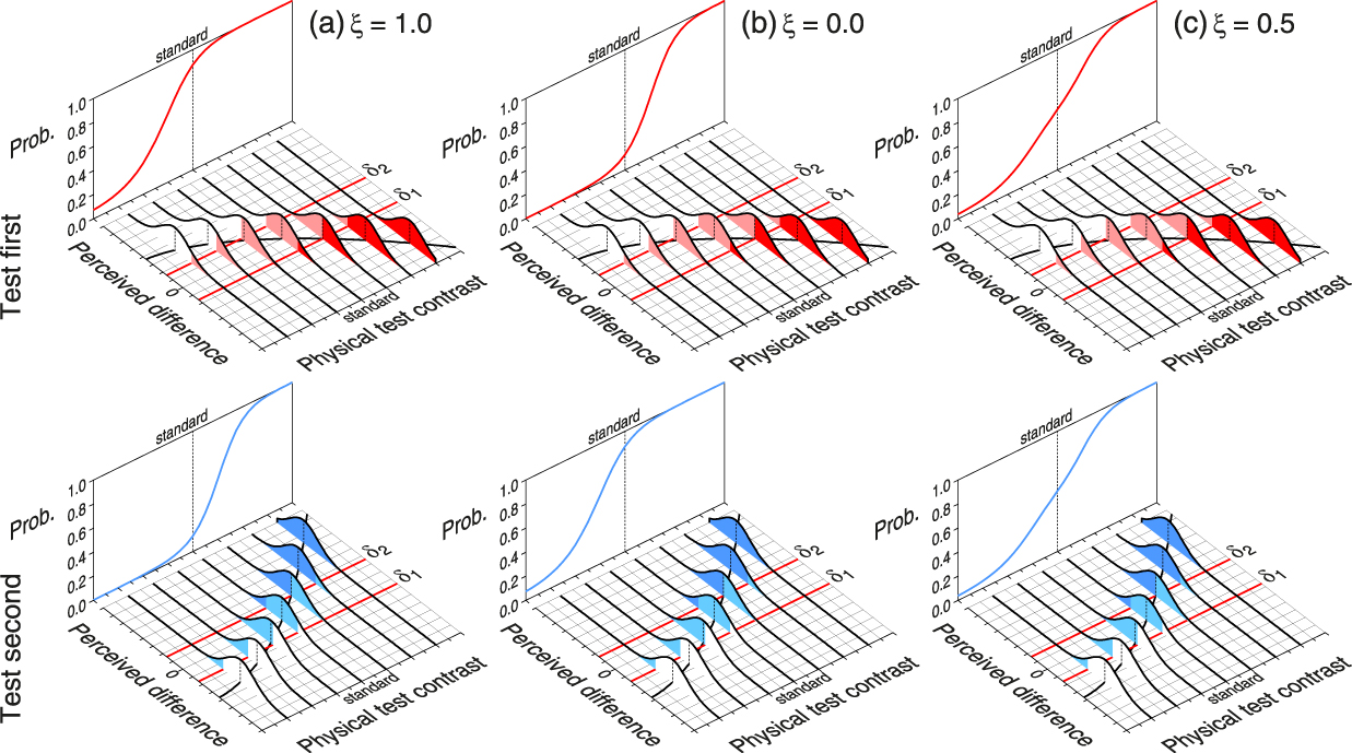
Figure 10. Psychometric Functions for “Test Higher” Responses under the Binary Response Format (i.e., Guessing when Uncertain) on Trials in which the Test Stimulus is Presented First (Top Row) or Second (Bottom Row), for Sample Values of the Probability ξ of Responding “First” when Guessing (Columns).
Areas marked in dark color indicate the probability of authentic “test higher” judgments; areas marked in light color indicate the probability of “equal” judgments that will or will not contribute to “test higher” responses according to the guessing strategy. (a) ξ = 1 so that all guesses result in “first” responses translating into “test higher” when the test is presented first and “test lower” when it is second. (b) ξ = 0 so that all guesses result in “second” responses translating into “test lower” when the test is first and “test higher” when it is second. (c) ξ = 0.5 so that half of the guesses result in “first” responses and the other half in “second” responses.
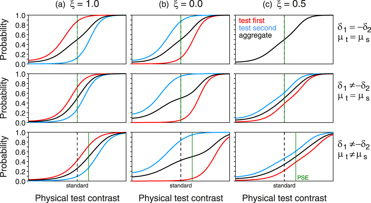
Figure 11. Psychometric Functions for “Test Higher” Responses under the Binary Response Format with Guessing on Trials in which the Test Stimulus is Presented First (Red Curve) or Second (Blue Curve) and also for Aggregated Data (Black Curve).
The three functions are identical and superimposed in the top-right panel. Functions are plotted for sample values of the probability ξ of responding “first” when guessing (columns) in three cases (rows). Top row: Centered interval of perceptual uncertainty and equal psychophysical functions for test and standard (i.e., the conditions in Figure 10). Center row: Displaced interval of perceptual uncertainty (in the form illustrated in Figure 8) still with identical psychophysical functions for test and standard. Bottom row: Displaced interval of perceptual uncertainty with unequal psychophysical functions for test and standard that shift the PSE (green vertical line) away from the standard magnitude (dashed vertical line).
This pattern is slightly different when the interval of perceptual uncertainty is not centered (i.e., when δ1 ≠ −δ2; see the red and blue curves in the center row in Figure 11) under otherwise identical conditions. Displacements across presentation orders still occur relative to the true PSE but now psychometric functions differ across presentation orders even when ξ = .5 (center panel in Figure 11c). They were identical in Figure 10c (and in the top panel of Figure 11c) because Eqs. 10a and 10b are identical when ξ = .5 and δ1 = −δ2. In general, psychometric functions for each presentation order are always displaced in opposite directions with respect to the true PSE by a distance that is null only when ξ = .5 and δ1 = −δ2. In passing, note that there is evidence of Ulrich and Vorberg’s (Reference Ulrich and Vorberg2009) Type B order effects in the center and bottom panels of Figure 11b, although we will defer commentary on this to the Discussion.
The second aspect that needs consideration is the consequences of aggregating data across presentation orders. To our knowledge, this was never done with ternary data except for summary purposes after psychometric functions for each presentation order had already been estimated (e.g., García-Pérez & Peli, Reference García-Pérez and Peli2014; Self et al., Reference Self, Mookhoek, Tjalma and Roelfsema2015). Then, here we will only illustrate the consequences of aggregating binary data collected with instructions to guess. Aggregation has indeed been the universal first step toward fitting a psychometric function, even years after the unacceptable consequences of this practice had been demonstrated by Ulrich and Vorberg (2009; see also García-Pérez & Alcalá-Quintana, Reference García-Pérez and Alcala-Quintana2011b) and despite the availability of user-friendly freeware to fit psychometric functions properly to data separated by presentation order (Bausenhart, Dyjas, Vorberg, & Ulrich, Reference Bausenhart, Dyjas, Vorberg and Ulrich2012; García-Pérez & Alcalá-Quintana, Reference García-Pérez and Alcalá-Quintana2017). It is clear that, at any test magnitude, the overall proportion of “test higher” responses equals the average of the proportions separately computed at each presentation order when the number of trials was the same under both orders. Then, averaging the psychometric functions in each column of Figure 10 renders the same result regardless of ξ (note that the black curves in all the panels in the top row of Figure 11 are identical). Yet, aggregation across presentation orders does not really remove the effects of ξ; it only standardizes the data to a putative ξ = .5 (as if guesses had been evenly split into “first” and “second” responses via Fechner’s strategy) but, again, only if δ1 = −δ2 as in Figure 10 or in the top row in Figure 11. As seen in Figure 11, the psychometric function for aggregated data (black curves) is not generally invariant with ξ and it also differs from the psychometric functions for each presentation order. The only invariant feature is that the psychometric function for aggregated data always has its 50% point at the true PSE, which may (top and center rows in Figure 11) or may not (bottom row in Figure 11) coincide with the standard magnitude contingent on whether or not µt = µs.
The picture just described is more complex when the number of trials administered at each individual test magnitude is not the same for both presentation orders (see Figure 13 in García-Pérez & Alcalá-Quintana, Reference García-Pérez and Alcalá-Quintana2011a), an unjustifiable practice when responses will be aggregated (which they should never be in the first place). In any case, note that aggregation does not misestimate the PSE although the artifactually reduced slope of the psychometric function misrepresents the true sensitivity of the observer. This explains why Lapid, Ulrich, and Rammsayer (2008, 2009; see also Rammsayer & Ulrich, Reference Rammsayer and Ulrich2012) found that the DL is generally smaller under the reminder task (i.e., all trials with test-second presentations) than it is under a procedure that they called 2AFC and involved a random mixture of trials with test-first and test-second presentations followed by aggregation of data to fit a single psychometric function. But this artifact does not mean that the observer’s sensitivity differs across tasks by sensory factors (i.e., due to the underlying psychophysical functions). Far from it, the sensory components of performance (including sensitivity) are identical and it is only the responses that are contaminated by irrelevant non-sensory factors that broaden the observed psychometric function for aggregated data. For further analyses and discussion of this issue, see García-Pérez and Alcalá-Quintana (Reference García-Pérez and Alcalá-Quintana2010b).
Empirical evidence supporting the indecision model
The foregoing presentation of the indecision model illustrated its capability to retrospectively account for general features that are inconsistent with the conventional framework routinely used to analyze and interpret data. The validity of the indecision model does not rest only on retrospective demonstrations but, more importantly, on evidence coming from research designed to check its assumptions and to test some specific and quite strong predictions. A few of those studies are briefly described next.
The indecision model predicts how observed psychometric functions in dual-presentation methods under the binary response format without allowance for “equal” responses should vary with the order of presentation of test and standard and, in turn, how these should additionally vary with the guessing strategy of the observer. These variations are predicted to occur without changes in the sensory parameters describing the psychophysical functions for test and standard. Thus, differences in observed performance across guessing strategies should be accounted for with common sensory parameters but suitably different decisional and response parameters. These predictions were supported in a within-subjects study on visual luminance contrast discrimination (with identical test and standard stimuli) in which psychometric functions for each presentation order were measured under response strategies involving always responding “first”, always responding “second”, or guessing evenly between the two upon judgments of equality (Alcalá-Quintana & García-Pérez, 2011). With intensive magnitudes such as luminance contrast, the use of identical test and standard stimuli does not necessarily ensure that the 50% point on the psychometric function will be at the standard magnitude. Procedural aspects such as the timing of presentations within or across trials may interfere with the natural processing of the stimulus in only one of the presentations, for instance by displaying a stimulus when an aftereffect from the preceding presentation has not yet washed out. If this happened within each trial but not across trials, the stimulus presented second (be it the standard or the test) would be functionally processed as if under a different psychophysical function. The study just mentioned also included another within-subjects factor with conditions that favored desensitization during the second presentation (via a short inter-stimulus interval), during the first presentation (via a short inter-trial interval), or in none of them (via long inter-stimulus and inter-trial intervals). The effects of desensitization (or lack thereof) on the observed psychometric functions for each presentation order were also well accounted for by the model, orthogonally with the effects of response strategy. At the early stage of development in which this study was conducted, the data were not analyzed under the indecision model as presented here but see Figure 20 in García-Pérez and Núñez-Antón (Reference García-Pérez and Núñez-Antón2018) for an analysis along those lines. Unpublished estimates of the sensory, decisional, and response parameters obtained by fitting the psychometric functions in Eqs. 8 and 9 above corroborated the validity of the indecision model.
Another strong tenet of the indecision model is that the psychophysical function for the stimulus dimension of concern should be estimated to be identical regardless of the psychophysical method used to collect the data and despite possible differences among the observed psychometric functions obtained with each method. The results presented earlier in Figure 7 for data collected with SJ2, SJ3, and TOJ tasks on the same observers and with the same stimuli support this prediction. As described there, differences among observed psychometric functions can be accounted for by differences in decisional and response parameters with no change in the parameters that describe how physical asynchrony maps onto perceived asynchrony and, thus, on the estimated location of the true PSS (not to be confused with the location of some landmark on an observed psychometric function).
Another test of the assumption of invariance of the psychophysical function was reported by García-Pérez and Peli (Reference García-Pérez and Peli2014), this time in a comparison of the outcomes of single- and dual-presentation methods in a spatial bisection task with the stimuli in Figs. 1a and 1b. The within-subjects study included single-presentation methods with the binary left–right and the ternary left–center–right response formats and a dual-presentation method in which observers reported either in which of the two presentations was the bar closer to the midpoint or else that they appeared to be equally close in both cases. The large within-subject variation in the presumed location of the bisection point observed across tasks was nevertheless accounted for by a unique psychophysical function that combined with task-specific decisional and response factors that distorted the shape of the observed psychometric function in each case. Two further aspects are worth mentioning regarding this empirical test. One is that, in the joint fit of the indecision model to data collected with the three methods, estimates of the parameters of the psychophysical function were obtained using data from the dual-presentation method, which is the only type of method that allows separating them from decisional and response parameters as discussed above. These estimates were inserted for estimation of the decisional parameters δ1 and δ2 for each of the single-presentation methods, which would have been impossible to estimate separately. The resultant estimates were not symmetrically placed with respect to the perceptual midpoint, which accounted for an otherwise incomprehensible lateral displacement of the psychometric functions obtained with single-presentation methods. The second aspect is that the response format in the dual-presentation version did not ask observers to compare bar positions but their absolute offsets (i.e., distance to the perceptual midpoint regardless of direction). Then, the relevant decision variable D is not the simple difference used thus far in our illustrations but D = |S 2| − |S 1|, whose distribution we will not reproduce here but is obviously non-normal (see Appendix A in García-Pérez & Peli, Reference García-Pérez and Peli2014).
In another study on invariance of the psychophysical function across procedural changes, García-Pérez and Alcalá-Quintana (Reference García-Pérez and Alcalá-Quintana2015c) reanalyzed data reported by Magnotti, Ma, and Beauchamp (Reference Magnotti, Ma and Beauchamp2013) on the perception of synchrony in audiovisual speech. Data had been collected with the SJ2 task in four within-subject conditions in which the auditory component of the stimulus was identical whereas the visual component was manipulated in two orthogonal ways. As discussed earlier (see Figure 7), the asymmetric Laplace distributions of perceived asynchrony assumed by the indecision model include components from each of the stimuli whose synchrony the observer judges. Because the auditory stimulus in Magnotti et al.’s study (2013) was the same in all conditions, its contribution to performance should have been identical across manipulations. Observed differences in the psychometric functions for “synchronous” responses across manipulations of the visual stimulus should thus be the result of differences in the visual component with an identical auditory component in all cases. The reanalysis confirmed that observed performance could be very accurately accounted for by the indecision model with invariant parameters for the auditory component in all conditions and parameters for the visual component that varied across conditions.
An intimately related issue arises when pairs of identical stimuli are used in these studies, such as two identical visual shapes asynchronously presented side by side on a monitor. This should imply identical components from both stimuli, unless the location of a stimulus on the visual field differentially affects its processing. The indecision model is a good tool to test the empirical question of whether or not such differences exist, by determining whether a variant with different parameters for each stimulus accounts for the data better than a variant with the same parameters for both. Reanalysis of several data sets from studies conducted by other researchers in these conditions and using both SJ2 and TOJ tasks in a within-subjects design (García-Pérez & Alcalá-Quintana, Reference García-Pérez and Alcalá-Quintana2015a, Reference García-Pérez and Alcalá-Quintana2015b) rendered two major conclusions. First, that estimating common parameters for both stimuli accounted for the data just as well as allowing different parameters for them, thus rejecting the hypothesis of differences in timing processes between visual hemifields. Second, and again, that performance in SJ2 and TOJ tasks can be described via common timing processes despite the disparate psychometric functions and (presumed) estimates of the PSS that each task provides.
The last piece of evidence that we will discuss relates to the consequences of a mismatch between the number of existing judgment categories and the number of options that the response format permits, in a way that judgment categories are collapsed differently under alternative response formats. A long-standing question in timing perception was whether perception of asynchrony is a sufficient or only a necessary condition for perception of temporal order. In the former case, observers should be able to report temporal order as soon as they notice an asynchrony whereas, in the latter, they may notice an asynchrony but still be unable to tell temporal order. If the latter were true, there should be an interposed region in decision space on each side of the central region for “synchronous” judgments, reflecting cases in which perceived asynchrony is sufficiently large for a judgment of asynchrony (as if out of the central region in one sense) but insufficient to identify temporal order (as if still inside the central region in another sense). These extra regions would give the impression of a shorter distance between δ1 and δ2 in SJ2 or SJ3 tasks (because they yield “asynchronous” responses in these tasks) than in TOJ tasks (because they yield guesses here). Some empirical evidence of this pattern of results had been reported (García-Pérez & Alcalá-Quintana, Reference García-Pérez and Alcalá-Quintana2015b) and data collected with a 4-ary SJ4 task in which a fourth response option was allowed to reflect this judgment confirmed its qualitatively distinct character and its occurrence at asynchronies that agree with expectations (García-Pérez & Alcalá-Quintana, Reference García-Pérez, Alcalá-Quintana, Vatakis, Balcı, Di Luca and Correa2018). It should be noted that the SJ4 task had been used earlier (see Weiß & Scharlau, Reference Weiß and Scharlau2011), but the conventional method with which the data were analyzed could only give inconclusive results.
Best practices and practices to be avoided
The foundation of this paper is that the psychometric function is not simply a mathematical expression conveniently fitted to data with the only purpose of extracting its slope and location but, rather, the observable manifestation of the interplay of sensory, decisional, and response processes which should be separated and extracted from the data. Decoding those influences requires fitting a process model of the psychometric function with explicit representation of the different components via functional parameters describing their operation. The preceding sections of this paper served two goals in this general context. One was to present empirical evidence questioning the validity of the conventional framework used to interpret psychometric functions measured with single- or dual-presentation methods. The other was to present an alternative framework explaining the anomalies that the conventional framework cannot account for and to discuss further empirical evidence supporting the validity of the alternative framework.
Analysis of the underpinnings and predictions of the indecision model has revealed that not all of the available psychophysical methods provide equally informative data and that not all the forms in which the data can be treated do justice to the processes that produced them. Five major practical recommendations arise from this analysis, which are summarized next along with a reminder of the reasons why such practices are or are not advisable.
1) Avoid single-presentation methods (see Figs. 5 and 6). Single-presentation methods confound sensory and decisional parameters in a way that the psychometric function is detached from the characteristics of the underlying psychophysical function and cannot be interpreted in perceptual terms. However, if the only goal of a study is to estimate sensitivity as indicated by the slope of the psychometric function irrespective of its location, then a single-presentation method is safe to use only if the response format allows an “undecided” response (in any suitable designation) so that guesses do not reduce the observed slope of the psychometric function artifactually.
2) Administer dual-presentation methods with allowance for “equal” responses, which implies using the ternary response format or, at least, the same–different format (see Figs. 8–11). Without allowance to report judgments of equality separately, observers would have to misreport them via guesses that make the data contain an unnecessary and undifferentiated mixture of authentic judgments and misreports. Random or systematic guessing always reduces the true slope of the psychometric function and shifts its location which, again, makes it uninterpretable in perceptual terms.
3) Never aggregate data across presentation orders (or positions) with the goal of estimating a single psychometric function to the aggregate (Figs. 8–11). Psychometric functions for each presentation order generally differ from one another due only to decisional and response factors. The slope of the psychometric function for aggregated data is not interpretable in perceptual terms because it has been artifactually reduced by those factors.
4) Fit psychometric functions to dual-presentation data separated by presentation order under a model-based approach with suitable parameters. As seen in Eqs. 8 and 9, psychometric functions for each presentation order or position imply the exact same parameters, namely, those in the psychophysical functions μs and μt (and those in σs and σt, if these variances are not constant) plus δ1 and δ2.
5) Collect data using adaptive methods that run separately for each presentation order and whose trials are randomly interwoven. We have not discussed sampling plans for the collection of data, as if using the method of constant stimuli as it is understood today (i.e., administering the same number of trials at each of a fixed set of predetermined test magnitudes) were appropriate. When psychometric functions for each presentation order are laterally shifted, the range of relevant test magnitudes is not the same for both orders and, thus, trials should be differently deployed for each order ensuring that the same numbers of trials are administered in each case.
Recommendations for the choice of psychophysical method and response format are easy to follow, as they only require enabling an additional response key to record “equal” responses and storing in the log file the order in which test and standard were presented in each trial. The same is true for the choice of optimal adaptive sampling plans (see García-Pérez, Reference García-Pérez2014b; García-Pérez & Alcalá-Quintana, Reference García-Pérez and Alcalá-Quintana2005). Finally, using the alternative framework for analysis of data and interpretation of the psychometric functions is just as easy with the freeware available for such purpose (Alcalá-Quintana & García-Pérez, Reference García-Pérez and Alcalá-Quintana2013; García-Pérez & Alcalá-Quintana, Reference García-Pérez and Alcalá-Quintana2017, Reference García-Pérez, Alcalá-Quintana, Vatakis, Balcı, Di Luca and Correa2018). The software fits model-based psychometric functions by estimating the relevant sensory, decisional, and response parameters and it also extracts from them the sought-after measures of performance for interpretation of the psychometric functions (PSE, PSS, DL, detection threshold, etc.).
As discussed above, fitting psychometric functions under this approach does not imply a multiplicity of parameters with which virtually anything will surely be fitted. Psychometric functions are not fitted separately for each presentation order each with its own parameters, but jointly with generally only three or four common parameters for them all. Nevertheless, there is an aspect of the response component that we have omitted in this paper, namely, the eventuality of response errors whereby judgments are sometimes misreported unintentionally, perhaps by hitting a wrong response key. Misreports often manifest as inexplicable responses such as “left” on a trial in which the vertical bar was actually far on the right and when the observer had actually responded “right” on every other trial with the bar at that location. When fitting conventional psychometric functions, response errors (lapses) are handled by addition of asymptote parameters. Such lapse parameters are also included in the response component of the indecision model and they can be estimated along the way if the data so requires (see Alcalá-Quintana & García-Pérez, Reference García-Pérez and Alcalá-Quintana2013; García-Pérez & Alcalá-Quintana, Reference García-Pérez and Alcalá-Quintana2017, Reference García-Pérez, Alcalá-Quintana, Vatakis, Balcı, Di Luca and Correa2018). It should be noted, though, that lapse parameters do not provide the model with the flexibility needed to fit data that it could not possibly fit otherwise. The model is sufficiently constrained to allow data to rule it out, and lapse parameters only permit a more accurate description of some aspects of the data (see, e.g., García-Pérez & Alcalá-Quintana, Reference García-Pérez and Alcalá-Quintana2012b).
Discussion
This paper has discussed the evidence that invalidates the conventional framework for interpretation of the psychometric function obtained with psychophysical methods involving single or dual presentations, has presented an alternative framework that is compatible with such evidence, and has discussed the way in which psychometric functions are fitted and interpreted under the alternative framework. The indecision model is an empirically-supported framework for the analysis and interpretation of psychometric functions whose main contribution is the separation of sensory, decisional, and response components of observed performance so that the effects of experimental manipulations can be attributed to the appropriate component, thus allowing a faithful characterization of sensory processes and an investigation of the locus of differences in observed performance. A number of issues mentioned only in passing throughout the paper are next discussed in some detail.
Is the indecision model the only alternative framework?
The fact that observers are sometimes undecided is an empirical truth acknowledged by all psychophysicists and routinely handled via instructions to guess. Amending the conventional framework by addition of an interval of perceptual uncertainty as the indecision model does seems a must not only to model guessing behavior adequately but also to allow accounting for performance in same–different tasks or their single-presentation analogues coherently. We have shown that this sole addition accounts for all the aspects of performance that the conventional framework can only regard as anomalies and, in the interest of parsimony, no extra assumptions should be incorporated. Nevertheless, this section briefly comments on two other alternatives that are not as comprehensive and that share two undesirable characteristics. One is their assumption that the psychophysical functions for standard and test are both the identity function μ(x) = x (i.e., a form of the phi-gamma hypothesis; see Thurstone, Reference Thurstone1928) so that they implicitly deny that the true PSE might lie away from the standard magnitude and they thus regard any semblance of it as constant error. The second one is that they focus on order effects and propose mechanisms that can only operate in dual-presentation methods, remaining silent about all the failures of the conventional framework for data collected with single-presentation methods.
Chronologically, the first alternative is the sensation-weighting model (Hellström, Reference Hellström1977, Reference Hellström1978, Reference Hellström1979, Reference Hellström1985, Reference Hellström2003; Hellström & Rammsayer, Reference Hellström and Rammsayer2015). Research under this model has never sought to model or check out the causes of constant errors, and psychometric functions have never been the subject of analyses analogous to those presented here. Yet, the main tenet of the sensation-weighting model can be paraphrased in terms of the conventional framework: Observers make their judgment according to a decision variable computed as D = w 2S 2 – w 1S 1, where w 1 and w 2 are the weights applied to the perceived magnitude in each presentation. In contrast, w 1 = w 2 = 1 under both the conventional framework and the indecision model. The assumption of a weighted difference could certainly be combined with those of the indecision model but it is noteworthy that sensation-weighting alone produces order effects even with a single boundary in decision space (for an illustration in the context of detection tasks, see Figure 5 in García-Pérez & Alcalá-Quintana, Reference García-Pérez and Alcalá-Quintana2011a). Application of the model has succeeded in finding weights w 1 and w 2 that provided a post hoc account of constant errors, but this model has two major drawbacks. One is that modelling “equal” responses requires an interval of perceptual uncertainty which is actually included in the model (but considered in only some of the studies) and whose functional interaction with sensation weighting makes the resultant model non-identifiable and useless for distinguishing decisional bias from perceptual effects: There are an infinite number of combinations of decision boundaries δ1 and δ2 and weights w 1 and w 2 that produce the exact same psychometric function. The second one is that, although the model can be successfully fitted to data, it is not at all clear that it is testable in the sense that one could first predict how certain manipulations would change the weights and then conduct a study to check it out, or predict how constant errors should or should not vary across changes in the response format or the response strategy.
The second alternative is the internal reference model (Lapid, Ulrich, & Rammsayer, Reference Lapid, Ulrich and Rammsayer2008; Bausenhart, Bratzke, & Ulrich, Reference Bausenhart, Bratzke and Ulrich2016; Bausenhart, Dyjas, & Ulrich, Reference Bausenhart, Dyjas and Ulrich2015; Dyjas & Ulrich, Reference Dyjas and Ulrich2014; Dyjas, Bausenhart, & Ulrich, Reference Dyjas, Bausenhart and Ulrich2012, Reference Dyjas, Bausenhart and Ulrich2014; Ellinghaus, Gick, Ulrich, & Bausenhart, Reference Ellinghaus, Gick, Ulrich and Bausenhart2019). This generative model resembles the conventional framework for dual-presentation methods in that the decision variable is also computed as an unweighted difference and in that the decision space has a single boundary β in the comparative task (i.e., observers are never uncertain and never judge equality in this task) although the model replaces it with possibly asymmetric boundaries δ1 and δ2 for the equality task. The difference with the conventional framework lies in what is compared to what. Rather than assuming that the stimulus presented second is compared to that presented first, the model assumes that D = S 2 – I i, where I i is the internal standard on trial i, a random variable defined as a convex combination of the random variable S 1 and the value I i−1 of the internal standard on the preceding trial. The comparison then uses a dynamically perturbed S 1 (even when the first stimulus is not the standard) with a distribution whose moments differ from those of S 2 even when both stimuli have identical magnitude and when psychophysical functions for test and standard are also identical (which is always true under this model by assumption). The distribution of the internal standard can be shown to differ when the standard or the test are presented first, which produces Type B order effects by altering the resultant slope of the psychometric function across presentation orders. On the other hand, Type A order effects are modeled as criterion bias whereby the single boundary in decision space is set at some β ≠ 0.
Two further comments seem necessary about this model. The first one relates to its applicability to single-presentation methods. For this purpose, Dyjas et al. (2012, p. 1833) described ad hoc assumptions which contradict those that hold for dual presentations about how the internal standard is updated and what it is compared to. Also, the context of their application is still that of dual-presentation methods, although the standard is presented only at the beginning of the session. Even a sole presentation of the standard at the beginning of the session prevents interpreting the psychometric function in terms of what it might have been without such presentation. The second comment regards empirical tests supporting this model, beyond the empirical fact that Type A and Type B order effects are found in the data. Only in two studies (Bausenhart et al., Reference Bausenhart, Dyjas and Ulrich2015; Ellinghaus et al., Reference Ellinghaus, Gick, Ulrich and Bausenhart2019) model psychometric functions were fitted to the data in search for a functional description of performance via model parameters, but the most common way in which the model has been “tested” (e.g., Dyjas et al., Reference Dyjas, Bausenhart and Ulrich2012, Reference Dyjas, Bausenhart and Ulrich2014) is by fitting arbitrary and general-purpose psychometric functions in search for differences in slopes and locations estimated without the constraints that the model imposes. This was also true in the only study (Dyjas & Ulrich, Reference Dyjas and Ulrich2014) in which the use of alternative response formats with a within-subjects design would have allowed a true test of the prediction that differences in observed performance across presentation orders and response formats can be accounted for with identical estimates of (at least some of the) internal reference model parameters.
How can the interval of perceptual uncertainty be displaced?
The indecision model allows boundaries δ1 and δ2 that are not symmetrically placed relative to a suitable anchor such as the perceptual midpoint in Figs. 5 and 6, perceptual synchrony in Figure 7, or the null difference in Figs. 8–11. This same allowance was included in the internal reference model when it was applied to equality tasks by Dyjas and Ulrich (Reference Dyjas and Ulrich2014) and to date it is the only mechanism that has been proposed to account for universally observed lateral shifts of the psychometric function across presentation orders or positions.Footnote 5 This allowance is obviously analogous to that for criterion bias in the conventional framework, consisting of permitting the single boundary β to move away from its suitable anchor.
It is unclear what mechanism would shift the interval of perceptual uncertainty, but it could be attentional or strategic in nature. For instance, the observer might focus finely on identifying a departure in one of the directions and report a departure in the other direction only when it is so conspicuous that it can be perceived inattentively. Luckily, this issue lends itself to investigation via manipulation of the observers’ strategies. It is also worth mentioning that a displaced interval was implicitly evident when Urban (1910, p. 250) wrote out the probability of an “equal” response as the area under the unit-normal distribution between the points  ${h_1}\left( {x - {a_1}} \right)$ and
  ${h_2}\left( {x - {a_2}} \right)$, where x is stimulus magnitude. The resemblance to Eqs. 8c and 9c above is obvious except that Urban displaced the limits of integration relative to an anchored distribution instead of displacing the distribution (via the psychophysical function) relative to fixed integration limits at δ1 and δ2. This observation supports our earlier statement that the indecision model is not a novel idea and it can be traced back to Urban over a century ago. In any case, what matters for the present discussion is that Urban did not impose any constraints on the free parameters a 1, a 2, h 1, and h 2 and, thus, the limits of integration could be asymmetrically placed. Urban seemed more concerned with discussing the implicit phi-gamma hypothesis than with offering a reason for asymmetric integration limits although he must have realized that symmetric limits could not possibly account for the ubiquitous constant error that he was seeing in the data.
What about Type B order effects in the indecision model?
We have not discussed Type B order effects in detail but it is important to realize that they can also occur under the indecision model. Figure 11 showed that the model can produce different slopes for the psychometric function across presentation orders under the binary response format with guessing, and Figure 8 also showed that these differences will also manifest under the ternary response format in which equality can be reported. Type B order effects may occur under the indecision model due to several factors. Type B order effects in Figs. 8 and 11 are caused by nonlinear psychophysical functions and the size of the effects is larger when the interval of perceptual uncertainty is not symmetric or when guesses are not evenly distributed under the binary response format without allowance to report equality (see García-Pérez, Reference García-Pérez2014a). All of this is consistent with the fact that the large differences in slope across presentation orders under the comparative task with guessing do not seem to have a counterpart under the equality task (see Dyjas & Ulrich, Reference Dyjas and Ulrich2014).
But there is a third factor that will produce Type B order effects, one whose identification can again be traced back to Urban (Reference Urban1910). Note that the upper and lower limits of integration in the expressions reproduced above are linear functions of (test) stimulus magnitude x but not necessarily with the same slope (i.e., there is no such constraint as h 1 = h 2). In terms of the indecision model, this comes down to making δ1 and δ2 depend on stimulus magnitude. One may surmise that, on any given trial, it is neither the magnitude of the standard nor that of the test that determines the values of δ1 and δ2 but, rather, the magnitude of the stimulus presented first, as if the observer set the operating resolution that is needed according to the perceived magnitude of the first presentation. For instance, the resolution that an observer needs to tell apart the second from the first presentation in a duration discrimination task is surely not the same when the duration of the first presentation is 50 ms than when it is 800 ms. In conditions in which the variance of perceived magnitude also increases with physical magnitude (as is the case in perception of duration), Type B order effects are predicted to occur.
What if I am not fitting psychometric functions or estimating psychophysical functions?
The short answer to this question is that the problems of interpretation under the conventional framework remain: The effects discussed here are always present in the data and they are not something that manifests only when psychometric functions are fitted to such data or when the researcher has certain goals. Several methods have been devised as shortcuts to estimate the location of thresholds, PSEs, or DLs without the burden of collecting enough data for explicitly fitting a psychometric function, but they all implement rules still grounded on the conventional framework and its assumptions (i.e., absence of judgments of equality and guessing, lack of order effects, and lack of criterion bias).
For illustration, consider the widely-used up–down staircases that seek to estimate some percentage-correct point on the monotone increasing psychometric function arising in tasks using the binary response format with guesses, an estimate obtained by averaging the test magnitudes at the reversal points. Staircase methods assume that the psychometric function is invariant so that the probability of a correct response at any given test magnitude x is always the same.Footnote 6 In dual-presentation methods, the order of presentation of the two stimuli in each trial is randomized and, in the presence of order effects, the assumption of invariance of the probability of a correct response at test magnitude x is thus violated. In practice, this means that data are collected in each trial at random from one of two different psychometric functions (according to which order of presentation was used in each trial) and the average-of-reversals estimate obtained in these conditions is thus devoid of meaning.
What about multiple-presentation methods?
We mentioned in the Introduction that multiple-presentation methods can be used and we confirm that the indecision model can equally be used to model performance on them. For instance, when three magnitudes are presented in each trial and the observer has to report which one is stronger, all current models effectively assume that the observer carries out as many sequential pair comparisons as necessary to finally judge which presentation displayed a stronger stimulus. Under the conventional framework, each of these pair comparisons involves a separate process as that illustrated in Figs. 3 or 4 but each of them is surely susceptible of rendering a judgment of equality that can be captured “as is” under the indecision model. In fact, order effects have also been described for multiple-presentation tasks (see, e.g., Johnson, Watson, & Kelly, Reference Johnson, Watson and Kelly1984; Kim, Lee, & Lee, Reference Kim, Lee and Lee2010). As sentenced in the Introduction, the extra burden of using more than two presentations per trial does not pay back with more informative data or more accurate parameter estimates, and it also has the drawbacks of calling for extra response parameters to deal with the multiplicity of forms in which undecided responses can occur across all the necessary pair comparisons and to model the process by which the response is given.


 Open access