


1. Introduction
This study develops and verifies a new spatial modeling method for cityscapes that can handle the features of the space, which is generally expressed separately as image information and geometric information of an image collectively, by using multiple deep learning techniques.
1.1. Image analyses for architecture and urban planning
In the fields of architecture and urban planning, analysis is commonly performed to examine the impression of space. For example, the sky ratio and greenery view index are commonly used; these metrics indicate the amount of visible sky (e.g., Kokalj, Zakšek, & Oštir, Reference Kokalj, Zakšek and Oštir2011) and amount of green (e.g., Li et al., Reference Li, Zhang, Li, Ricard, Meng and Zhang2015), respectively. To conduct such research, a comprehensive image database linked to a map is required. Because large-scale image data, such as street view (SV) are available, image analysis is becoming feasible. For example, research studies with Google Street View (GSV) by Gebru et al. (Reference Gebru, Krause, Wang, Chen, Deng, Aiden and Fei-Fei2017), Rzotkiewicz et al. (Reference Rzotkiewicz, Pearson, Dougherty, Shortridge and Wilson2018) and Steinmetz-Wood, Velauthapillai, & O’Brien (Reference Steinmetz-Wood, Velauthapillai and O’Brien2019). In general, when image analysis method for spaces is conducted, meaningful and calculable features must be extracted from the images in advance. However, since space has not only such colour and texture characteristics but also has various geometric characteristics as described in Section 1.2; features that affect the impression of space are not always exhaustive and could not thus be defined explicitly.
In recent years, there have been rapid advances in convolutional neural networks (CNN; Karpathy, Reference Karpathy2019). These networks, which automatically extract features from images are used for classification, regression and other tasks. CNNs have become a fundamental technology in the field of artificial intelligence because, unlike conventional statistical analysis and machine learning methods, CNNs automatically learn image data features, thereby eliminating the need to prepare features in advance and creating new tasks, such as object detection and semantic segmentation (SS) and highly accurate recognition. Given these advantages, CNNs have been increasingly applied to various fields, even in the spatial analysis of cities. For example, CNNs have been applied to the SS task, which classifies images into a finite number of labels by pixel. With a CNN, SS accuracy has improved to the extent that the results can be applied to practical situations. Helbich et al. (2019) applied SS to a SV image, extracted the quantity corresponding to the above-mentioned greenery view index and examined the relationship to depression. Fu et al. (Reference Fu, Jia, Zhang, Li and Zhang2019) extracted greenery, sky and building view indexes using SS for SVs in large cities in China and analysed the relationship between these indexes and land prices. Yao et al. (Reference Yao, Zhaotang, Zehao, Penghua, Yongpan, Jinbao, Ruoyu, Jiale and Qingfeng2019) proposed a method to predict the relationship between a human examiner’s space preference results and the quantity of some components by machine learning by applying SS to urban SV images.
These studies use images of urban space as explanatory variables by labelling major components. However, as mentioned above, the quality of urban space cannot be explained entirely by such explicit features. The biggest advantage of deep learning is that the feature quantity can be extracted automatically. A previous study by Liu et al. (Reference Liu, Silva, Wu and Wang2017) exploited the advantages provided by deep learning. They conducted an impression evaluation experiment of SVs in Chinese city space, performed by experts and predicted the impression directly from SV images using a representative CNN, such as AlexNet (Krizhevsky, Ilya, & Geoffrey, Reference Krizhevsky, Ilya and Geoffrey2012). Seresinhe, Preis, & Moat (Reference Seresinhe, Preis and Moat2017) also explored whether ratings of over 200,000 images of Great Britain from the online game, Scenic-Or-Not (Data Science Lab, n.d.), combined with hundreds of image features extracted using the Places Convolutional Neural Network (Zhou et al., Reference Zhou, Lapedriza, Xiao, Torralba and Oliva2014), in order to understand what beautiful outdoor spaces are composed of. Law, Paige, & Russell (Reference Law, Paige and Russell2019) showed that land prices could be estimated with higher accuracy than general GIS data by extracting features from London SV and satellite images using a simple CNN with a hedonic model.
1.2. Isovist versus image analysis for spatial analysis
As described above, many studies have been investigated using CNNs and SVs and various approaches have been developed. However, all these studies use standard angle-of-view images. An image of space is considered suitable for capturing colour and textural features of space. However, geometric features, such as openness and size are also important for space. Conventionally, these features have been studied using a space analysis method called Space Syntax (Hillier & Hanson Reference Hillier and Hanson1989). Geometric features handled by space syntax are mainly calculated from the depth of space. On the other hand, current image analysis method like SS divides each pixel of an image into a belonging class. That is, SS can extract geometric features related to the shape of objects but not depth information.
Among spatial analysis methods of space syntax, an isovist (Benedikt, Reference Benedikt1979) is fundamental and important as a model expressing local features of space. A single isovist shows a polygon in the case of two-dimensions (see Figure 1) or a polyhedron in the case of three-dimensions of the visible area or volume, which can be viewed from a vantage point. There have been many studies dealing with the two-dimensional isovist since it was proposed by Benedikt. For example, Batty (Reference Batty2001) proposed various spatial feature quantities, such as mean distance and area of the two-dimensional isovist. Ostwald & Dawes (Reference Ostwald and Dawes2018) have clarified that there is a correlation between human behaviour and isovists.
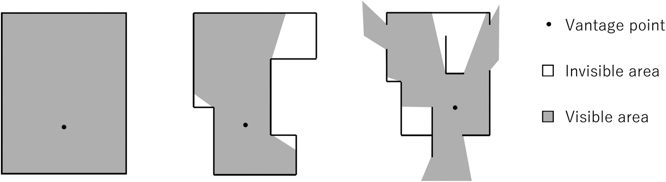
Figure 1. Example of two-dimensional isovists.
Recently, the research on extracting and utilizing the three-dimensional (3D) isovist has increased (Chang & Park Reference Chang and Park2011; Garner & Fabrizio Reference Garnero and Fabrizio2015; Lonergan & Hedley Reference Lonergan and Hedley2016; Krukar et al. Reference Krukar, Schultz and Bhatt2017; Kim, Kim, & Kim, Reference Kim, Kim and Kim2019), since performance improvement of the computer and utilization of the 3D space data have become easy. In the case of the two-dimensional isovist, geometrically exact shape of the isovist can be obtained by using an algorithm based on the plane scanning method (Suleiman et al. Reference Suleiman, Joliveau and Favier2012). On the other hand, in the case of 3D isovist, since the calculation method for obtaining its exact shape becomes complicated, some approximate methods have been generally used. Among them, the method, which approximately obtains the 3D isovist as a set of visual lines radiated omnidirectionally from a vantage point at a fixed angle and they touch the nearest obstacle, is widely used. Here, we call such isovist as ‘approximate isovist’.
Figure 2 illustrates an isovist and visual lines for creating the approximate isovist. This approximate isovist is equivalent to adding the value of the length of each visual line as depth to the intersection of the line and a small projected sphere centred on the vantage point. In computer graphics, the depth of the space seen from a camera can be obtained very quickly from the pipeline of a graphics processing unit (GPU) as a depth map. When the camera is rotated to the vantage point as much as necessary, and the depth map obtained at every angle is projected on the sphere, the information equivalent to the approximate isovist can be obtained without generating visual lines. In this way, Chirkin, Pishniy, & Sender (Reference Chirkin, Pishniy and Sender2018) proposed a real-time method for obtaining the approximate 3D isovist and its feature quantities at the same time by using a GPU.
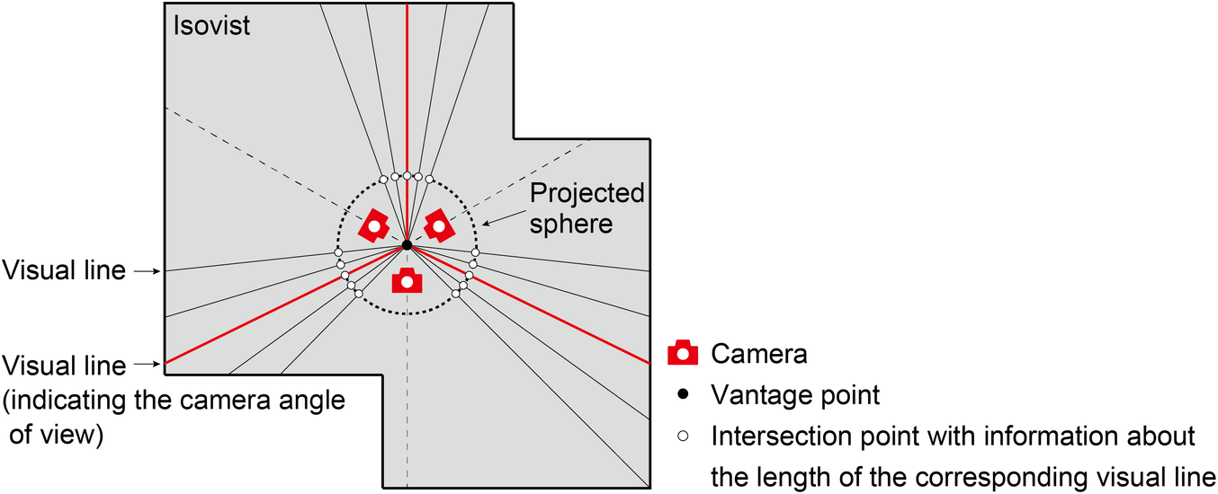
Figure 2. An isovist, finite visual lines for creating its approximate isovist and its projection on a sphere with cameras.
Although the technology to obtain an isovist has steadily evolved as just described, since an isovist itself can be considered a mold of the space, it can easily become a complicated shape, and the approach that clarifies the feature quantity of the shape has the same limitation as the image analysis. The problems associated with complicated shapes become particularly significant with the 3D isovist. However, the depth maps projected on the sphere can be used as an omnidirectional depth map. An omnidirectional image is generally saved as equal rectangular projection. In this paper, we call the usual omnidirectional image in Red-Green-Blue (RGB) format simply as an ‘omnidirectional image’ and corresponding omnidirectional depth map as a ‘depth map’. By using a CNN, it is possible to directly input the omnidirectional depth map itself without clarifying the feature quantity of the isovist necessary for an analysis until now. In addition, it opens up the possibility of constructing a model that naturally combines the depth map and corresponding omnidirectional RGB image.
Based on the above background, Takizawa & Furuta (Reference Takizawa and Furuta2017) captured a large number of omnidirectional images and their depth maps in a virtual urban space constructed using the Unity game engine (Unity Technologies, 2019) in real time. Then, using these images as input data, they constructed a model to predict the results of the preference scoring experiment of a virtual urban landscape with a CNN. Their results revealed that adding depth maps to ordinal omnidirectional images made it possible to construct a CNN with higher precision and easier interpretation. However, in that study, the quality of the virtual space used was low, and the preference scoring experiment was conducted only in the virtual space in which the generation of the depth map was easy but not in the real world.
1.3. Purpose
In this study, we developed a method to generate omnidirectional depth maps from corresponding omnidirectional images of cityscapes by learning each pair of images created by CG using pix2pix (Isola et al. Reference Isola, Zhu, Zhou and Efros2017), a general-purpose image translation method based on deep learning. Another method for performing image translation using GAN, such as pix2pix, there is CycleGAN (Zhu et al., Reference Zhu, Park, Isola and Efros2017). pix2pix is different from CycleGAN, in that it learns pairs of one-to-one images, while CycleGAN learns two sets of unpaired images. We use pix2pix because only one depth map corresponds to its RGB image.
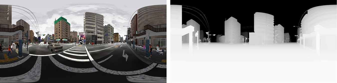
Figure 3. Omnidirectional image (left) and corresponding depth map (right) of a cityscape in a computer graphics model (©NONECG).
Then, models trained with different series of images, shot under different site and sky conditions, were applied to the omnidirectional images of GSV to generate their depth maps. The validity of the generated depth maps was then evaluated quantitatively and visually. In addition, we conducted preference scoring experiment of GSV images using multiple participants. We constructed a model that predicts the preference label of these images with and without the depth maps using the classification method with CNNs for general rectangular images and omnidirectional images. The results demonstrate the extent to which the generalization performance of the preference prediction model changes depending on the type of convolutional models, and the presence or absence of depth maps. Finally, we evaluated the efficiency of the proposed method.
This study was developed from our previous study (Kinugawa & Takizawa, Reference Kinugawa and Takizawa2019). The main differences from the previous study are the introduction of CNNs corresponding to omnidirectional images, as well as general rectangular images, the accuracy evaluation of generated depth maps and the change of the preference prediction problem to a simple classification problem. By these modifications, this paper intends to validate the proposed method more strictly.
1.4. Related studies
Recently, in relation to research into autonomous vehicles, methods to estimate the depth map of a given space from conventional images in RGB format without using a laser scanner have been investigated. This type of research is categorized by the number of cameras and whether the camera is moving or stationary. We deal with the problem of estimating depth map from a single RGB image taken by a monocular and still camera. Similar studies have been conducted by Saxena et al. (Reference Saxena, Chung and Ng2005) using a Markov random field, Mancini et al. (Reference Mancini, Costante, Valigi and Ciarfuglia2016) using a deep neural network, Hu et al. (Reference Hu, Ozay, Zhang and Okatani2018) using a CNN and Pillai, Ambru, & Gaidon (Reference Pillai, Ambru and Gaidon2019) tried super resolution depth estimation. However, only Zioulis et al. (Reference Zioulis, Karakottas, Zarpalas and Daras2018) dealt with omnidirectional images. Since that study focuses on estimating the depth of indoor images, it is unclear whether it is applicable to the street spaces that are the focus of this study.
The SYNTHIA dataset, developed by Ros et al. (Reference Ros, Sellart, Materzynska, Vazquez and Lopwz2016), is a pioneering attempt to generate artificial images, including omnidirectional depth maps, of a large number of urban landscapes, using CG to train a deep learning model. However, there are several differences between their study and the present study. Specifically, our study targets cityscapes in Japan and the shooting height of an image was set to the height of the GSV on-board camera, which is 2.05 m (Google Japan, 2009). In addition, only the depth map of the built and natural environment without cars and pedestrians is required. Thus, we can construct a unique dataset of urban spaces and use it for learning depth maps. Law et al. (Reference Law, Seresinhe, Shen and Gutierrez-Roig2018) also generated a virtual 3D city model using a software called Esri City Engine (ESRI, 2013) and took many cityscape images. Then, these images were learned by the CNN model and image classification of GSV was carried out. Their study is similar to our study, in that it applies models learned with a lot of synthetic images of street space to GSV images.
1.5. Organization of the paper
The remainder of this paper is organized as follows. The next section explains the proposed method. Next, the results of the proposed method are described through learning pix2pix and applying it to GSV images used for the experiment of preference scoring. Then, the results are discussed, and conclusions and suggestions for future work are presented.
2. Proposed method
The framework of the proposed method is shown in Figure 4. The proposed method is roughly divided into two parts. First, a CG-based urban space model is prepared. Omnidirectional images and depth maps are captured in real time in a virtual space and their pair images are collected. Using pix2pix, a model to generate the depth map from an omnidirectional image is constructed. Then preference scoring experiments of the cityscape images of GSV in Japan is conducted. For each omnidirectional image of GSV used for the experiment, its depth map is generated using the pix2pix model learned in the previous part and, after filtering the noise by SS, a four-channel Red-Green-Blue-Depth (RGBD) image is produced. The usefulness of the depth maps is verified by classification models, which predict the class label of the preference of the GSV images.
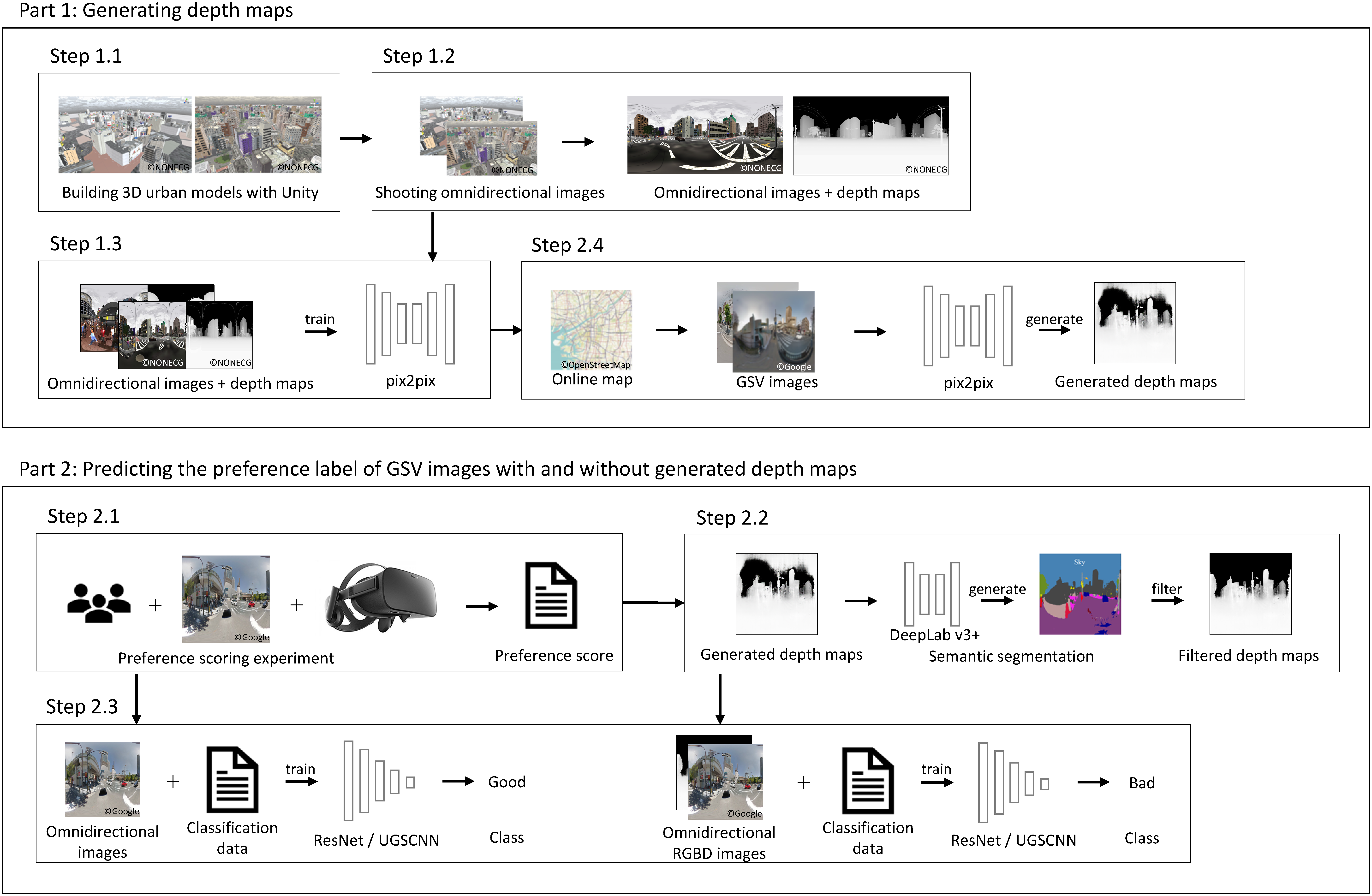
Figure 4. Framework of the proposed method.
2.1. Part 1: generating depth maps
The following is a step-by-step explanation of our research method.
Step 1.1: Building 3D urban space models
As used in previous studies (Takizawa & Furuta, Reference Takizawa and Furuta2017; Kinugawa & Takizawa, Reference Kinugawa and Takizawa2019), the game engine Unity was used to develop 3D models of the target city. In this study, we used two 3D urban models available from commercial CG content providers that are realistic and faithful to the actual Japanese urban space. The urban models used include the Shibuya model (NoneCG, n.d.), which simulates the central zone of the Shibuya area and a local city model (NoneCG, n.d.), which simulates a suburban district in Japan (Figure 5). To apply GSV images to the trained model, we added pedestrian and car models to the street and attempted to reproduce an actual urban space. Because the area of the original 3D models was not sufficiently wide to shoot depth maps, each model was copied and the street area was expanded multiple times. As mentioned previously, to acquire only the fixed spatial information of the built and natural environment, the depth maps used as training data excluded objects that may have served as obstacles in the space, such as pedestrians and cars. In addition, because actual photos of streetscapes vary greatly depending on weather, season and time, even for a single location, we used the Unity game engine’s Tenkoku Dynamic Sky (Tanuki Digital, n.d.) weather asset to modify the environmental conditions. Specifically, because sky conditions greatly affect the generation of depth maps, two sky conditions, that is, blue and cloudy were considered.
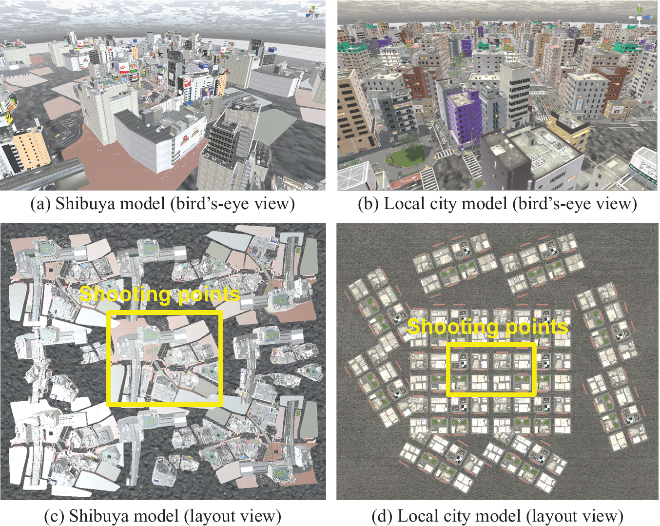
Figure 5. Two city models for training pix2pix (©NONECG).
Step 1.2: shooting omnidirectional images
For each of the two city models, the camera height was set to 2.05 m, which is the height of the GSV shooting car’s camera in Japan as described in Section 1.4. Next, as shown in Figure 6, a planar image of a 3D model was input to the GIS and a large number of shooting locations were randomly set on the road from the center area of the space (see Figure 5) with 500 points for each model. As described in Step 1.1, each urban model is created by copying the original 3D model and pasting it around to obtain a perspective image. Even if the number of shooting points is increased in the surrounding space, a similar close-up image is obtained and a sufficient distant view cannot be obtained. Therefore, the shooting points are set only in the center of the space.
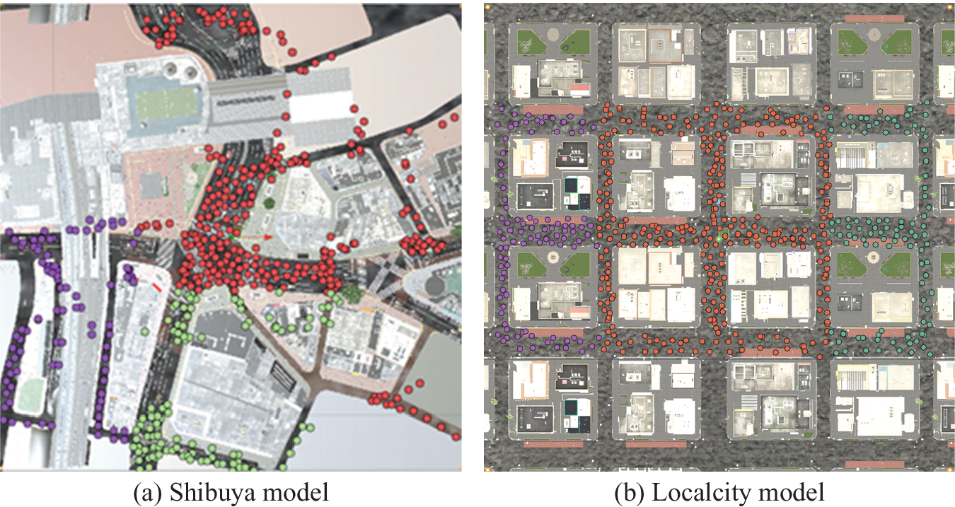
Figure 6. Shooting points in each city model. Red points are for training, green ones are for validation and purple ones for test (©NONECG).
The coordinates of the shooting points were imported into Unity and an omnidirectional image and its depth map were captured at each point. To capture omnidirectional images, we used a camera asset of Unity called Spherical Image Cam (which is no longer available). The number of the original dataset was increased by shooting 20 omnidirectional images by rotating the camera 18° at a single point. As a result, we obtained 20 × 500 = 10,000 images for each 3D model. The rotation operation of an image is a kind of data augmentation technique for image and essentially new information is not added. However, on a general CNN assuming rectangular images such as pix2pix, since large change of pixels at the right and left boundary of an image to be replaced by the rotation operation occurs, improvement on robustness of the model learned by these images can be expected.
For learning pix2pix, we split the datasets into training, validation and test set, the numbers of which are 300, 100 and 100 respectively, and coloured red, green and purple, respectively, in Figure 6. They are coloured with red, green and purple, respectively, in Figure 6. Spatial data have spatial auto-correlation and adjacent data often have similar features. In the case of CG images, in this study, since the distance to an adjacent shooting point is close to several meters, the problem of spatial autocorrelation cannot be ignored. Therefore, if images are randomly divided into learning, validation and test ones without considering the position of shooting points, similar images could be mixed in each data set. As a result, while validation and test become easy, realistic accuracy evaluation becomes hard. Therefore, the space is largely divided for each data set. The comparison of the generalization performance with the model based on the general randomization, which does not consider the spatial property may become a theme to be studied in future. Figure 7 shows an example of the image shoot in a local city model. The upper image is the original omnidirectional image and the lower part is the images cut by the general angle of view.
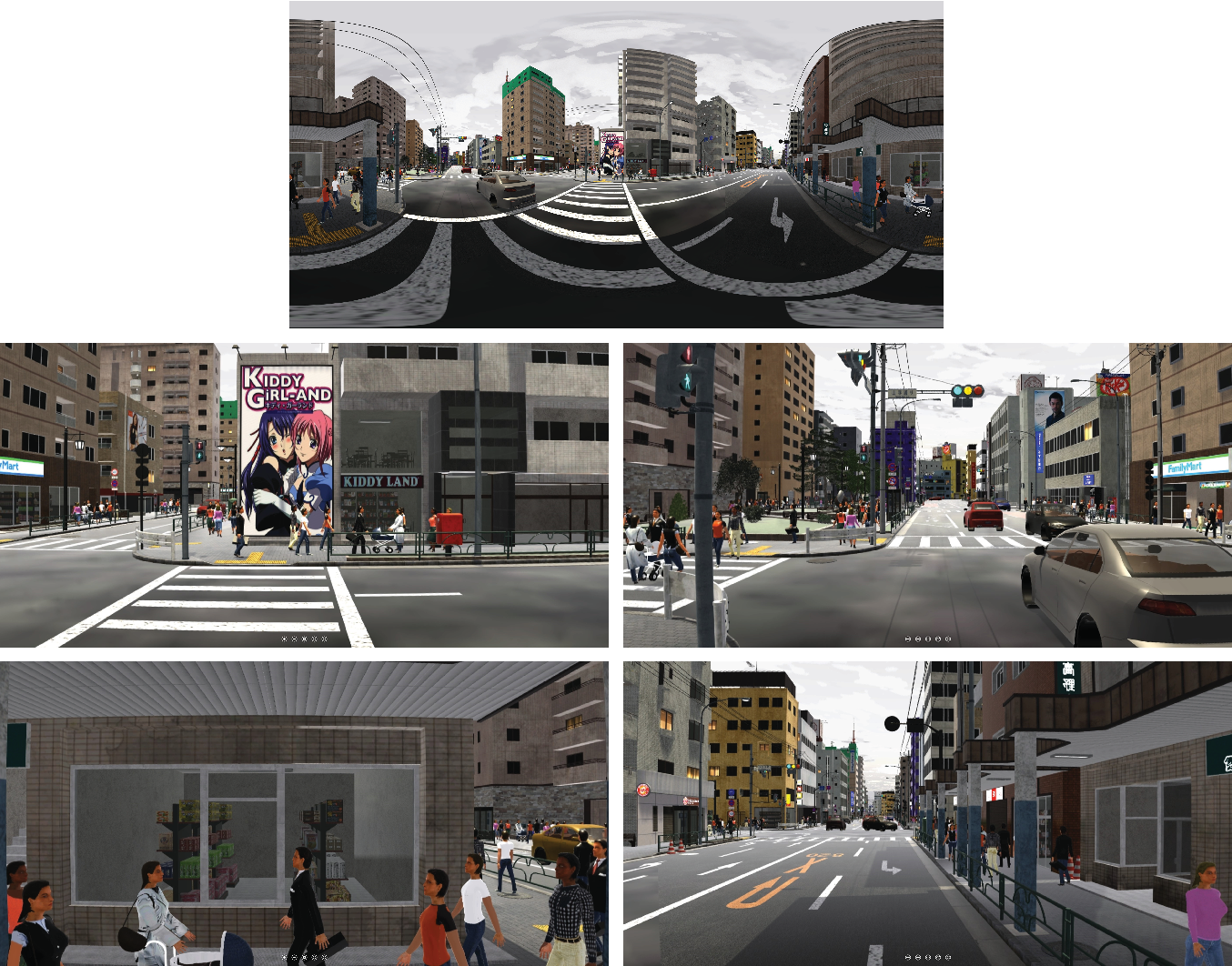
Figure 7. An omnidirectional image of local city model (top) and its four-way images at normal angle of view (©NONECG).
For generating a depth map from the depth buffer of a GPU, it is necessary to decide to what extent the depth is measured and distance conversion function to be used. Human sensory scales are often approximated by logarithmic scales but when we try to functionalize them with a logarithmic function, we need to determine some parameters. Therefore, we simply assume a linear function for distance. Since the information quantity per channel of a general image is eight-bit (i.e., 256 gradations), the resolution of the distance becomes coarse when the maximum distance is set long. To determine the critical distance, depth maps were generated with the maximum values of 100, 250 and 500 m as shown in Figure 8. In the depth maps, white colour denotes the depth is 0 and black colour denotes the depth is the maximum distance. The depth per 1 pixel value in each maximum value is 0.39, 0.98 and 1.96 m, respectively. When these figures are compared, there are differences in resolution for near objects and in recognition range for far objects, as well as there is a trade-off between them. The space handled in this study is mainly urban area and objects tend to concentrate in comparatively short distance. Therefore, this time, the limit distance was set to the shortest 100 m and the distance images were generated.
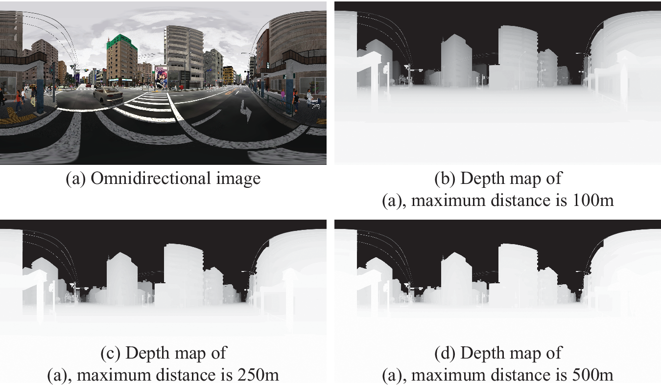
Figure 8. Comparison of shades of depth maps at different maximum distances (©NONECG).
Step 1.3: Implementing datasets for pix2pix and learning
Using pix2pix, we trained the model to generate depth maps from the omnidirectional images. pix2pix is an image translation model based on deep learning that generates images by learning the relationship between pairs of images. pix2pix comprises a generator (
 $ G $
) that generates an image and a discriminator (
$ G $
) that generates an image and a discriminator (
 $ D $
) that discriminates whether the image is real or fake (Figure 9). In addition, pix2pix is a type of deep learning method to generate images called conditional generative adversarial networks (conditional GAN) (Mirza & Osindero, Reference Mirza and Osindero2014). A conditional GAN learns mapping from input image,
$ D $
) that discriminates whether the image is real or fake (Figure 9). In addition, pix2pix is a type of deep learning method to generate images called conditional generative adversarial networks (conditional GAN) (Mirza & Osindero, Reference Mirza and Osindero2014). A conditional GAN learns mapping from input image,
 $ x, $
and noise vector,
$ x, $
and noise vector,
 $ z, $
to output image,
$ z, $
to output image,
 $ y, $
by
$ y, $
by
 $ G $
, that is,
$ G $
, that is,
 $ G:\left\{x,z\right\}\to y $
. The difference between the conditional GAN and pix2pix is that the latter generates the corresponding image based on the relationship between pair images while the conditional GAN generates the corresponding image based on the noise. pix2pix does not use a noise vector but it uses dropout, which randomly inactivates some nodes in training for relaxing overfitting, instead. The pix2pix loss function is the weighted sum of the loss function of the conditional GAN (
$ G:\left\{x,z\right\}\to y $
. The difference between the conditional GAN and pix2pix is that the latter generates the corresponding image based on the relationship between pair images while the conditional GAN generates the corresponding image based on the noise. pix2pix does not use a noise vector but it uses dropout, which randomly inactivates some nodes in training for relaxing overfitting, instead. The pix2pix loss function is the weighted sum of the loss function of the conditional GAN (
 $ {\mathcal{L}}_{cGAN} $
) and the L1 error between
$ {\mathcal{L}}_{cGAN} $
) and the L1 error between
 $ x $
and
$ x $
and
 $ y $
(
$ y $
(
 $ {\mathcal{L}}_{L1}\Big) $
. The L1 error prevents blurring of the generated image. Let
$ {\mathcal{L}}_{L1}\Big) $
. The L1 error prevents blurring of the generated image. Let
 $ {G}^{\ast } $
be the pix2pix loss function. Together with the other loss functions, they are given by the following formula where
$ {G}^{\ast } $
be the pix2pix loss function. Together with the other loss functions, they are given by the following formula where
 $ \lambda $
is a hyperparameter that determines which loss is more important. Note that
$ \lambda $
is a hyperparameter that determines which loss is more important. Note that
 $ \lambda $
was set to 100, which is the same value used in our initial study.
$ \lambda $
was set to 100, which is the same value used in our initial study.
 $$ {\mathcal{L}}_{cGAN}\left(G,D\right)={E}_{x,y}\left[\log D\left(x,y\right)\right]+{E}_{x,z}\left[\log \Big(1-D\left(x,G\left(x,z\right)\right)\right], $$
 $$ {\mathcal{L}}_{L1}(G)={E}_{x,y,z}\left[{\left\Vert y-G\left(x,z\right)\right\Vert}_1\right], $$
 $$ {G}^{\ast }=\arg \underset{G}{\min}\underset{D}{\max }{\mathcal{L}}_{cGAN}\left(G,D\right)+\lambda {\mathcal{L}}_{L1}(G). $$
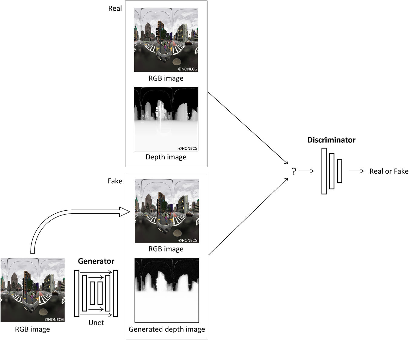
Figure 9. Outline of pix2pix process.
Here,
 $ D $
attempts to make the correct veracity decision as much as possible. On the other hand,
$ D $
attempts to make the correct veracity decision as much as possible. On the other hand,
 $ G $
avoids the correctness of the judgment as much as possible and attempts to match the original image with the generated image to some extent. These objectives are set alternately to learn the model parameters.
$ G $
avoids the correctness of the judgment as much as possible and attempts to match the original image with the generated image to some extent. These objectives are set alternately to learn the model parameters.
pix2pix uses U-Net (Ronneberger et al. Reference Ronneberger, Fischer and Brox2015) as an image generator. U-Net captures both the local and overall features of an image. In addition, pix2pix does not judge the authenticity of the whole image, rather it divides the image into several patches, evaluates the authenticity of the patches and finally judges the average of all patches to improve learning efficiency. This process is called patchGAN. In our implementation of pix2pix, the input image size is 256 × 256 pixels and the input images are divided into same 70 × 70 patch images, which are of the same size as the original pix2pix paper (Isola et al. Reference Isola, Zhu, Zhou and Efros2017).
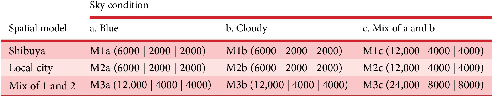
We prepared three types of spatial datasets for learning: Shibuya, a local city and a mix of the Shibuya and local city datasets. We also prepared three sky conditions: blue, cloudy and a mix of blue and cloudy. By combining the datasets, we generated nine training datasets, as listed in Table 1. As a reference, we add a supplementary file (supplement_a.pdf), including sampled 48 pairs of omnidirectional images, and their depth maps shoot in each city model on each sky condition as a supplemental material.
Table 1. Nine models used for training; In each cell, M__ denotes a model name and lower values denote the number of training data/validation data/test data.
Finally, to evaluate the generalization performance of pix2pix, the error at the pixel level for the correct image of the generated image is evaluated by root mean squared error (RMSE). Let
 $ X,Y,Z $
denote the ordered input image set, output image set and noise data set, respectively,
$ X,Y,Z $
denote the ordered input image set, output image set and noise data set, respectively,
 $ n $
denote the number of images in a data set and
$ n $
denote the number of images in a data set and
 $ m $
denote the number of pixels in an image. RMSE for each generated image
$ m $
denote the number of pixels in an image. RMSE for each generated image
 $ G\left(x\in X,z\in Z\right) $
and corresponding output image
$ G\left(x\in X,z\in Z\right) $
and corresponding output image
 $ y\in Y $
at the pixel is defined as follows:
$ y\in Y $
at the pixel is defined as follows:
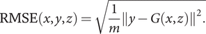 $$ \mathrm{RMSE}\left(x,y,z\right)=\sqrt{\frac{1}{m}{\left\Vert y-G\left(x,z\right)\right\Vert}^2.} $$
Then, we obtain mean RMSE for all images
 $ X,Y,Z $
as follows:
$ X,Y,Z $
as follows:
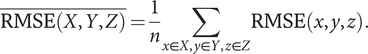 $$ \overline{\mathrm{RMSE}\left(X,Y,Z\right)}=\frac{1}{n}\sum_{x\in X,y\in Y,z\in Z}\mathrm{RMSE}\left(x,y,z\right). $$
The procedure of the accuracy evaluation is to obtain mean RMSE of the validation data for each pix2pix model learned by the designated epoch unit. Then, the depth maps are generated from the test data by the model of the epoch, whose value is minimum, and the mean RMSE is obtained and regarded as the generalization performance of the model.
Step 1.4 Generating GSV depth maps with the learned pix2pix
We input the omnidirectional GSV images to the trained pix2pix model and obtained a generated depth map. As described in 4.1, although the depth maps exist in GSV, the generated depth map of GSV cannot be evaluated by RMSE since the depth maps of GSV are practically useless. Therefore, we visually evaluated how realistic the generated depth map is. A total of 100 images were used to generate depth maps and the preference experiment described in Step 2.1. Fifty GSV images were sampled from both a local area (Neyagawa and Sumiyoshi) and an urban area (Umeda and Namba), respectively. Both areas were located in the Osaka Prefecture.
2.2. Part 2: predicting the preference class of GSV images using estimated depth maps
Using the estimated depth images, we predicted the preference label of the GSV images.
Step 2.1: preference scoring experiment
Each GSV image described in Section 1.4 was projected via an Oculus Rift, and a preference scoring experiment was conducted to generate the classification model. The cityscape of the collected GSV images was evaluated as good = 4, moderately good = 3, moderately bad = 2 and poor = 1. Twenty university students majoring in architecture were selected as participants, and each participant evaluated 50 GSV images from all 100 images. Note that participant fatigue was considered. Each image was presented to exactly 10 participants. Of the 20 participants, six were undergraduate students and 13 graduate students majoring in interior and housing design, and the other was a graduate student majoring in urban planning. Although all participants are involved in the design of space in a broad sense, the design of urban-scale space, in this study, is mostly out of the field. When we imagine the situation in which the preference prediction system of cityscape is used, the standard of the preference scoring seems to be different by the evaluator. We considered that it was better not to give bias to the preference scoring, and carried out the preference scoring experiment without clarifying the standard of the preference.
Figure 10 shows an example of an image of the GSV projected. The upper image is the original omnidirectional image and the lower part is the images cut by the general angle of view. Of course, the image that moves to the head-mounted display becomes a visually natural image, such as the lower one, depending on the viewing direction.
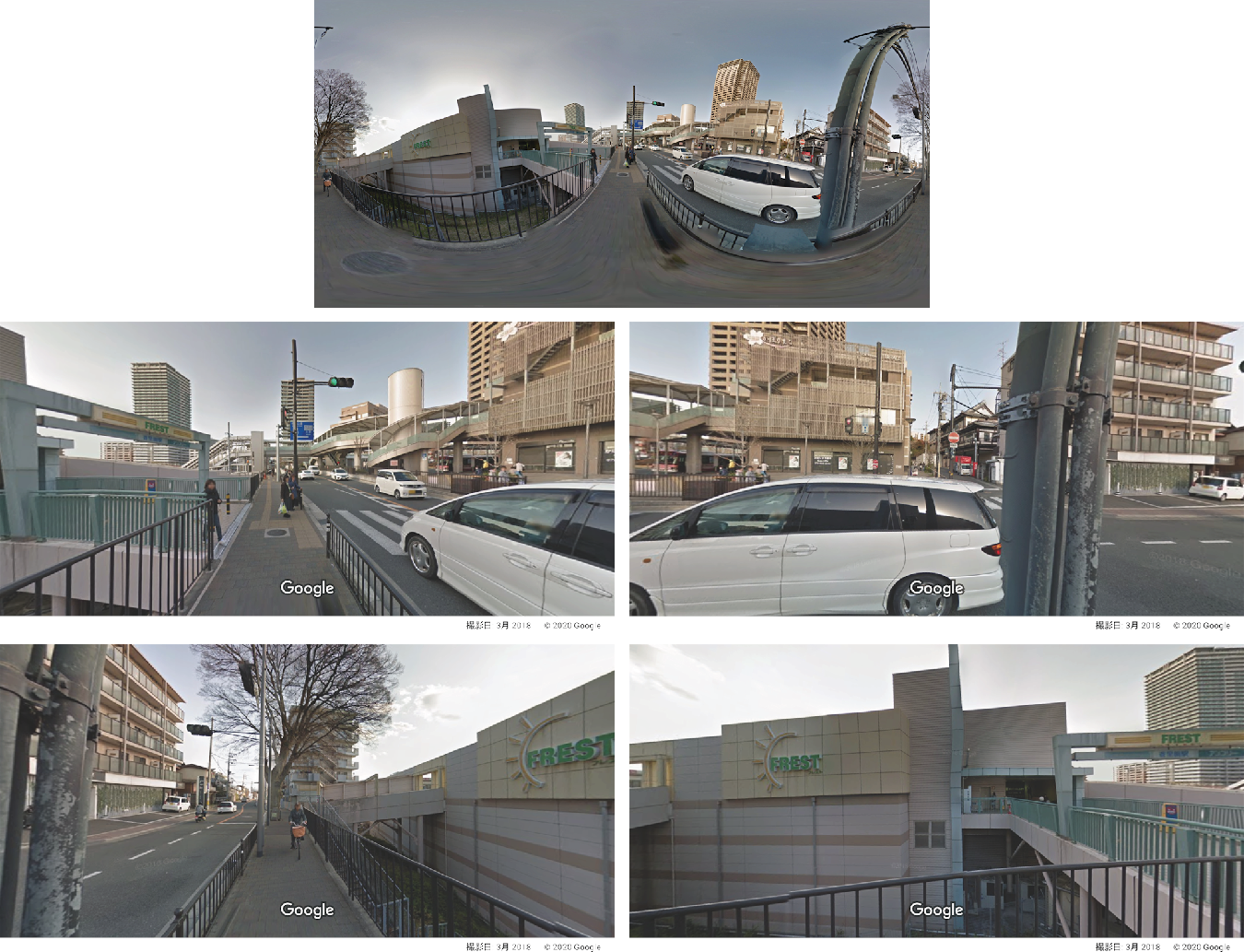
Figure 10. An example of an omnidirectional image of GSV (top) and its four-way images at normal angle of view (©Google, 2020).
Step 2.2: generation and filtering of RGBD images from GSV
Using the trained depth map generation models by pix2pix described above, depth maps were generated for each of the 100 GSV images used in the preference scoring experiment. Generating depth maps was performed using the M2c model, as it produced superior results by visual observation (Step 1.4). However, the sky area was estimated incorrectly (Figure 11b); therefore, the sky area of 9(a) was extracted by SS 9(c) and the value of the corresponding pixel was changed to black 9(d). For the SS model, the xception71_dpc_cityscapes_trainval model (Tensorflow, n.d.) of DeepLab v3+ (Chen et al., Reference Chen, Zhu, Papandreou, Schroff and Adam2018) was used. The outline of DeepLab v3+ is described in the appendix.
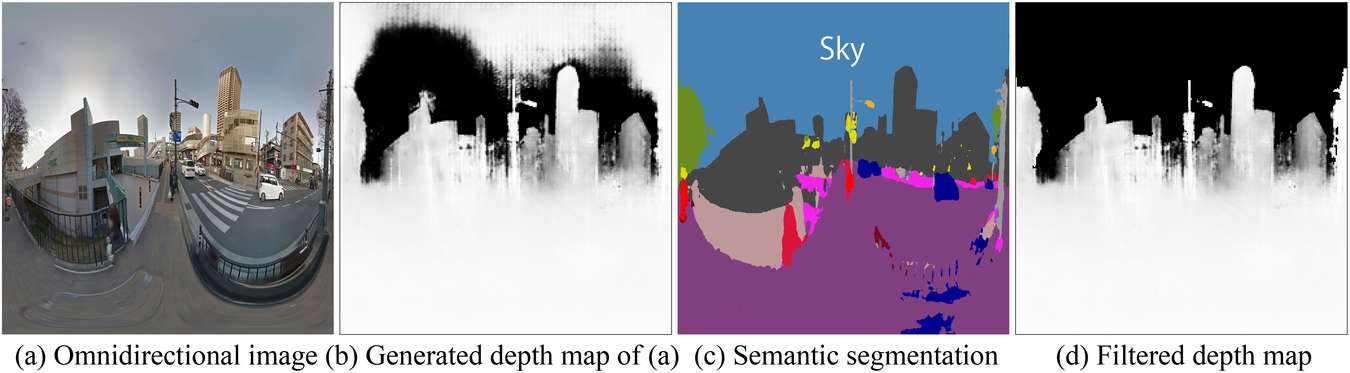
Figure 11. Filtering operation of a generated depth map for sky area using SS with the image of GSV (©Google, 2020).
When we use filtered depth maps, the omnidirectional images of the original GSV in RGB format were converted to RGBA format with 4 eight-bit channels and were resized to 256 × 256 pixels for ResNet (He et al., Reference He, Zhang, Ren and Sun2016) and 512 × 256 pixels for UGSCNN (Jiang et al., Reference Jiang, Huang, Kashinath, Prabhat, Marcus and Niessner2019) described in Step 2.3. Then, the depth value of the corresponding filtered depth map was stored to the A channel of the RGBA format image, thereby creating an RGBD image.
Step 2.3: classification model for estimating subjective preference using CNNs for rectangular and omnidirectional images
We construct CNN models that predict each preference label obtained in the preference scoring experiment using those RGB and RGBD images of GSV. In the preliminary experiment, the preference prediction model was defined and learned as a regression model with the mean of the preference score as an objective variable but the predicted score tended to gather around the mean value and the performance of the regression model was difficult to understand, therefore the preference prediction model is defined as a classification model. Although the validity of modeling the preference scores in two classes remains controversial, this study aims to model the preference in the framework of the simplest two-class classification problem. As future works, there remain studies such as introducing a classification problem of three classes of bad, moderate and good, and devising a way of giving training data to a regression model so that the above-mentioned problem of concentration of prediction scores hardly occurs.
For the classification model, ResNet, for the rectangular image and UGSCNN, which shows good performance in current spherical CNNs (Taco et al., Reference Taco, Mario, Jonas and Max2018) are used and the accuracy is compared.
ResNet model
We used ResNet-50 pretrained with ImageNet (Deng et al., Reference Deng, Dong, Socher, Li, Li and Fei-Fei2009) on 1000 classes and performed learning by fine-tuning all of model parameters. However, we modified the ResNet-50 input and output layers slightly. The number of channels of the image input layer was changed from three to four because an RGBD image has four channels. After the pretrained weights with RGB images were loaded, the layer was replaced. Therefore, the weights of not only D channels but also RGB channels were randomly initialized for the input layer. Furthermore, because our model is a two-class classification model, we changed the final layer of Resnet-50, which is composed of all connected layers with 1000 output nodes, to with two output nodes (Figure 12). The reason why the number of classes (i.e., preference rank) is set to two instead of four is described in Section 3.4.
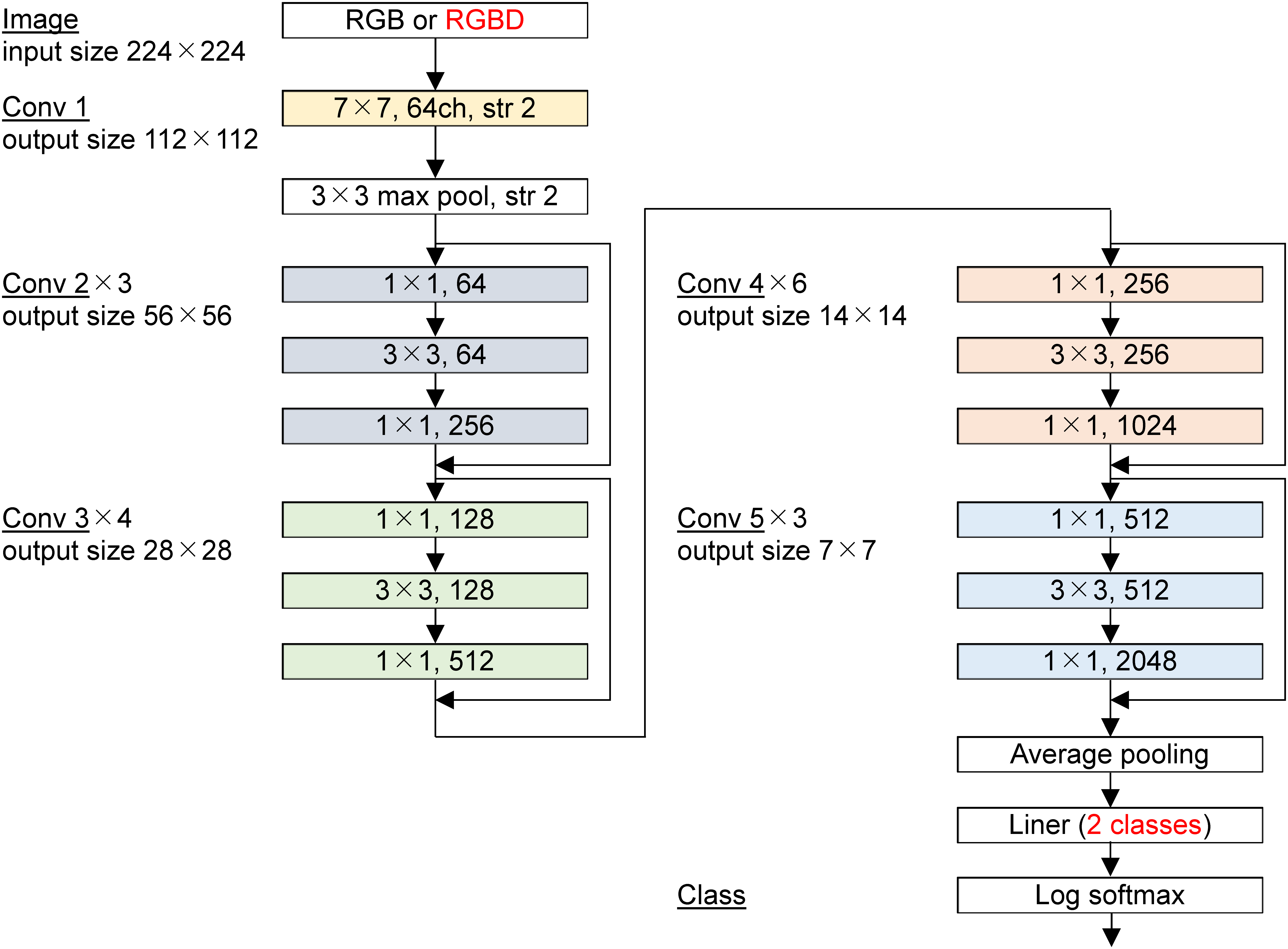
Figure 12. Modified Resnet-50 for RGB/RGBD image. The first and last parts noted in red are modified from original ResNet-50.
Although the number of GSV images was increased by 40 times by data augmentation, the original number of GSV images is 100 images, and there are few objective variables for learning a complex CNN model. As a result, the risk of over-fitting might increase. ResNet-152 was used for CNN in our past study (Kinugawa & Takizawa, Reference Kinugawa and Takizawa2019), but, in this study, the CNN was changed to ResNet-50 in which the number of parameters is about 40 % of ResNet-152 in order to reduce the risk of the over-fitting.
UGSCNN model
UGSCNN is a spherical CNN based on a polyhedron subdivided from a regular icosahedron. We used UGSCNN among some spherical CNNs proposed recently (Cohen et al., Reference Cohen, Geiger, Köhler and Welling2018; Coors, Condurache, & Geiger, Reference Coors, Condurache and Geiger2018; Tateno, Navab, & Tombari, Reference Tateno, Navab and Tombari2018) since UGSCNN is relatively new and has good performance. As illustrated in Figure 13, to each vertex of a polyhedron constituted by subdividing a regular icosahedron, information of pixels of a corresponding image is allocated by spherical mapping.
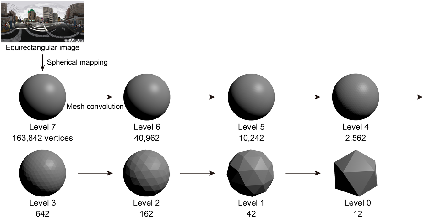
Figure 13. Mesh convolution of UGSCNN.
Then, mesh convolution is performed to convolve the information of each vertex and its adjacent vertices and the level of the polyhedron is reduced by one step. The division level of the icosahedron is set to 0 and the level increases one by one every time the subdivision is carried out and each time the polyhedron approximates a sphere. In this study, a mesh with a level of 7 was used as an initial polyhedron and mesh convolution was repeated until the level became 1. Referring to the example (exp2_modelnet 40) attached to the implementation of UGSCNN (maxjiang93, 2019), a CNN illustrated in Figure 14 was defined and used for classification.
Figure 14. UGSCNN used in this study.
To perform spherical mapping of an equirectangular image, the original RGB and RGBD images are resized to 512 × 256. Then, let
 $ \left(\lambda, \varphi \right) $
radians denote the pair of longitude and latitude of each vertex of the polyhedron, and
$ \left(\lambda, \varphi \right) $
radians denote the pair of longitude and latitude of each vertex of the polyhedron, and
 $ \left(x,y\right) $
denote the pair of the plane coordinate of a pixel of the image. The corresponding values of both coordinate systems are given by the following equations, where
$ \left(x,y\right) $
denote the pair of the plane coordinate of a pixel of the image. The corresponding values of both coordinate systems are given by the following equations, where
 $ round\left(\right) $
is a function that returns an integer rounded to the nearest whole number.
$ round\left(\right) $
is a function that returns an integer rounded to the nearest whole number.
 $$ x=255\bullet round\left(\lambda \right), $$
 $$ y=255\bullet round\left(\varphi \right). $$
Loss function
With the above CNN settings, we learn the two-class classification problem. The cross-entropy is used for the loss function. Let
 $ I $
denote the image dataset of GSV,
$ I $
denote the image dataset of GSV,
 $ J\in \left\{\mathrm{Bad},\mathrm{Good}\right\} $
denote the set of class labels,
$ J\in \left\{\mathrm{Bad},\mathrm{Good}\right\} $
denote the set of class labels,
 $ {y}_i\in J $
denote the class label of image
$ {y}_i\in J $
denote the class label of image
 $ i\in I $
,
$ i\in I $
,
 $ {\hat{y}}_{ij}\in \mathbb{R} $
denote the output of the log-softmax function of class
$ {\hat{y}}_{ij}\in \mathbb{R} $
denote the output of the log-softmax function of class
 $ j\in J $
of image
$ j\in J $
of image
 $ i\in I $
through a CNN. In 100 images of GSV, since the number of images of each class Bad and Good is 54 and 46, respectively, the images are not heavily skewed to one class. However, considering that the accuracy of the model is finally evaluated using the F1 score, which balances the number of data of each class, the learning is carried out with the following weights in order to give the effect that the number of data of each class becomes equal. Let
$ i\in I $
through a CNN. In 100 images of GSV, since the number of images of each class Bad and Good is 54 and 46, respectively, the images are not heavily skewed to one class. However, considering that the accuracy of the model is finally evaluated using the F1 score, which balances the number of data of each class, the learning is carried out with the following weights in order to give the effect that the number of data of each class becomes equal. Let
 $ {w}_j $
denote the weight of class
$ {w}_j $
denote the weight of class
 $ j\in J $
for relaxing the imbalance of image size for each class. That is, the learning is performed so that the loss of the minor class becomes relatively large. Let
$ j\in J $
for relaxing the imbalance of image size for each class. That is, the learning is performed so that the loss of the minor class becomes relatively large. Let
 $ {I}_j\subset I $
denote the image dataset of class
$ {I}_j\subset I $
denote the image dataset of class
 $ j\in J $
. Weight
$ j\in J $
. Weight
 $ {w}_j $
of class
$ {w}_j $
of class
 $ j\in J $
is given by
$ j\in J $
is given by
 $$ {w}_j=\frac{\min \left(\left|{I}_{\mathrm{Bad}}\right|,\left|{I}_{\mathrm{Good}}\right|\right)}{\left|{I}_j\right|}. $$
Finally, the loss function is given by
 $$ \mathrm{loss}=-\frac{1}{\sum_{i\in I}{w}_{y_i}}\sum_{i\in I}{w}_{y_i}{\hat{y}}_{ij}. $$
3. Results
Here, we describe the results of the proposed method.
3.1. Result of learning pix2pix (Step: 1.3)
We used the PyTorch implementation (Junyanz, n.d.) of pix2pix for training and verification. To improve learning speed and performance in different areas of CG and real images, we changed batch size from 1 to 50 and normalization method from batch normalization to instance normalization; however, the other pix2pix hyperparameter default values were used. These learning settings of pix2pix are summarized in Table A1 in Appendix.
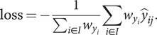
We performed learning for each model. In this study, we confirmed the accuracy of the model from the convergence of the loss function of the generator and discriminator. Figure 15 presents an example of the convergence of the loss function when M2c was trained up to 200 epochs. In Figure 15, G_L_cGAN equals
 $ {\mathcal{L}}_{cGAN}\left(G,D\right) $
and G_L_L1 equals
$ {\mathcal{L}}_{cGAN}\left(G,D\right) $
and G_L_L1 equals
 $ {\mathcal{L}}_{L1}(G) $
. D_Real and D_Fake are the cross-entropy loss of the discriminator when an actual image and generated image are input, respectively. As the epoch progresses, the losses of the discriminator decrease almost monotonically. On the other hand, the L1 loss of the generator takes a constant value after about 50 epochs. The GAN loss increases as the epoch progresses, which is a general tendency of a GAN learning process.
$ {\mathcal{L}}_{L1}(G) $
. D_Real and D_Fake are the cross-entropy loss of the discriminator when an actual image and generated image are input, respectively. As the epoch progresses, the losses of the discriminator decrease almost monotonically. On the other hand, the L1 loss of the generator takes a constant value after about 50 epochs. The GAN loss increases as the epoch progresses, which is a general tendency of a GAN learning process.
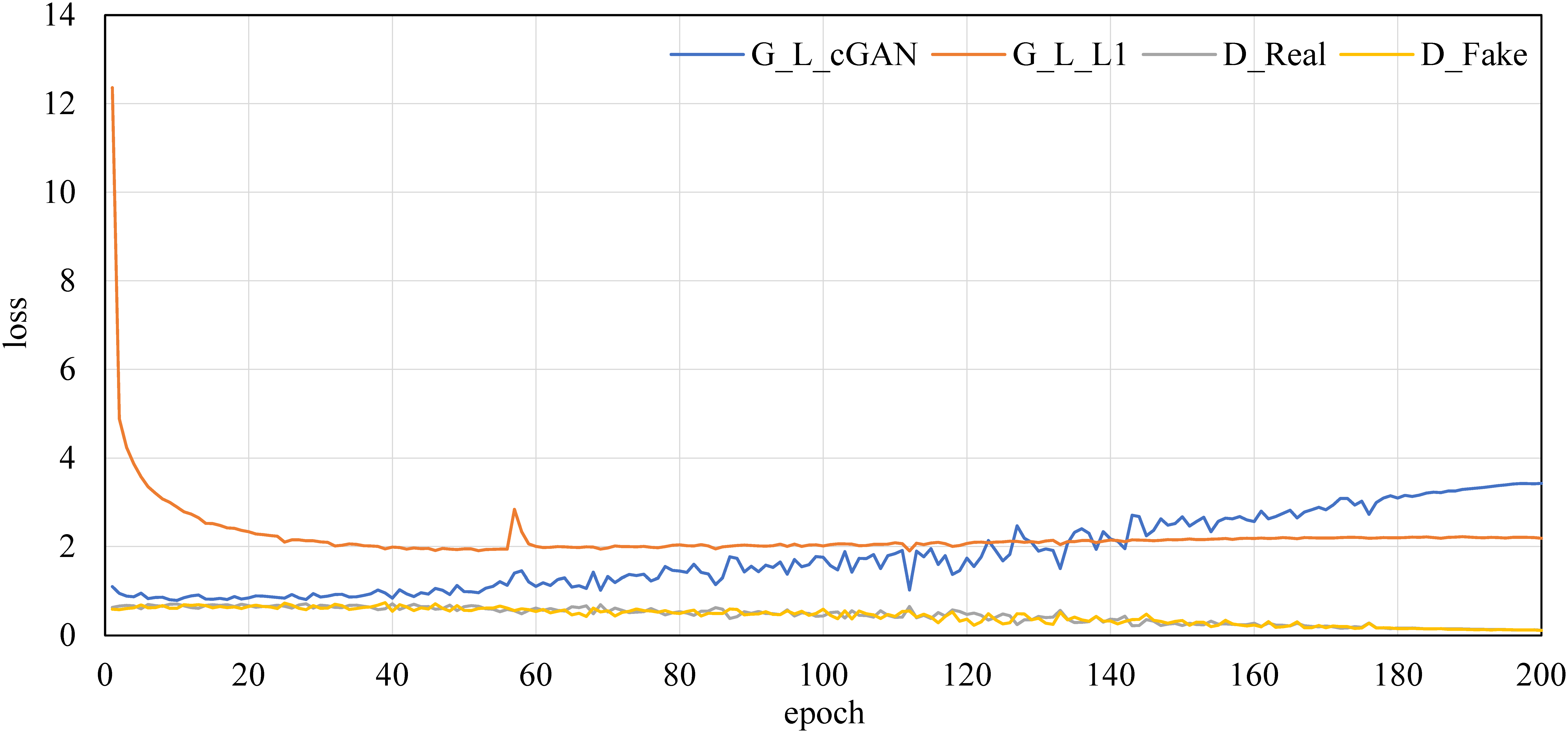
Figure 15. Example of convergence process of loss functions (M2c).
Table 2 lists RMSE of test data generated by each pix2pix model. Test data of each model and M3c with the most various kinds of images were used. The mean error is about five pixel values and the error is about 2 m when it is converted into the distance. An example of a generated depth map of a test data is shown in Figure 16. Since the error is relatively low and visual similarity is high, it is concluded that the distance estimation by pix2pix has high generalization performance in the case of same domain images.
Table 2. RMSE of test data generated by each pix2pix model.
Bold is the best value.
Figure 16. Example of a generated depth map of a test data (©NONECG) by M2c, RMSE = 4.37.
3.2. Result of verification of trained pix2pix model by GSV (Step: 1.4)
Comparison of depth maps of a GSV generated by each model is presented in Figure 17. The common feature is that relatively reasonable depth maps can be generated when the sky is cloudy or mixed whereas the depth maps generated by the model trained with clear sky images are not practical.
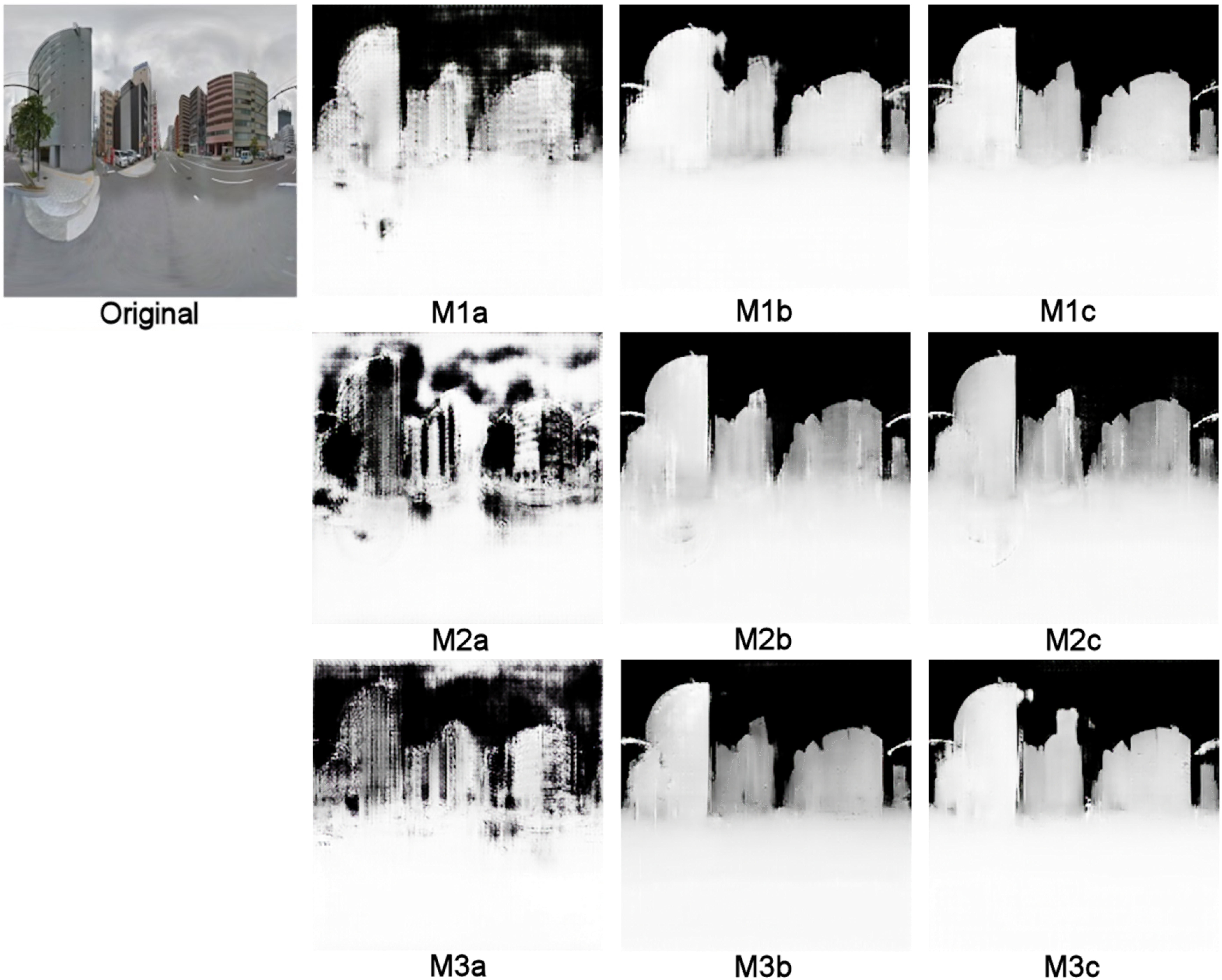
Figure 17. Comparison of depth maps of the same GSV image (©Google, 2020) generated by each model.
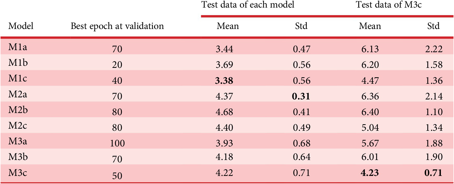
Since the most visually valid result was the result by M2c for 100 images of GSV, the depth map generated by M2c is used in the following. Figure 18 shows examples of depth maps of GSV images generated by M2c and their filtered depth maps. We also give all generated and filtered depth images of GSV as a supplementary material (supplement_b.pdf).
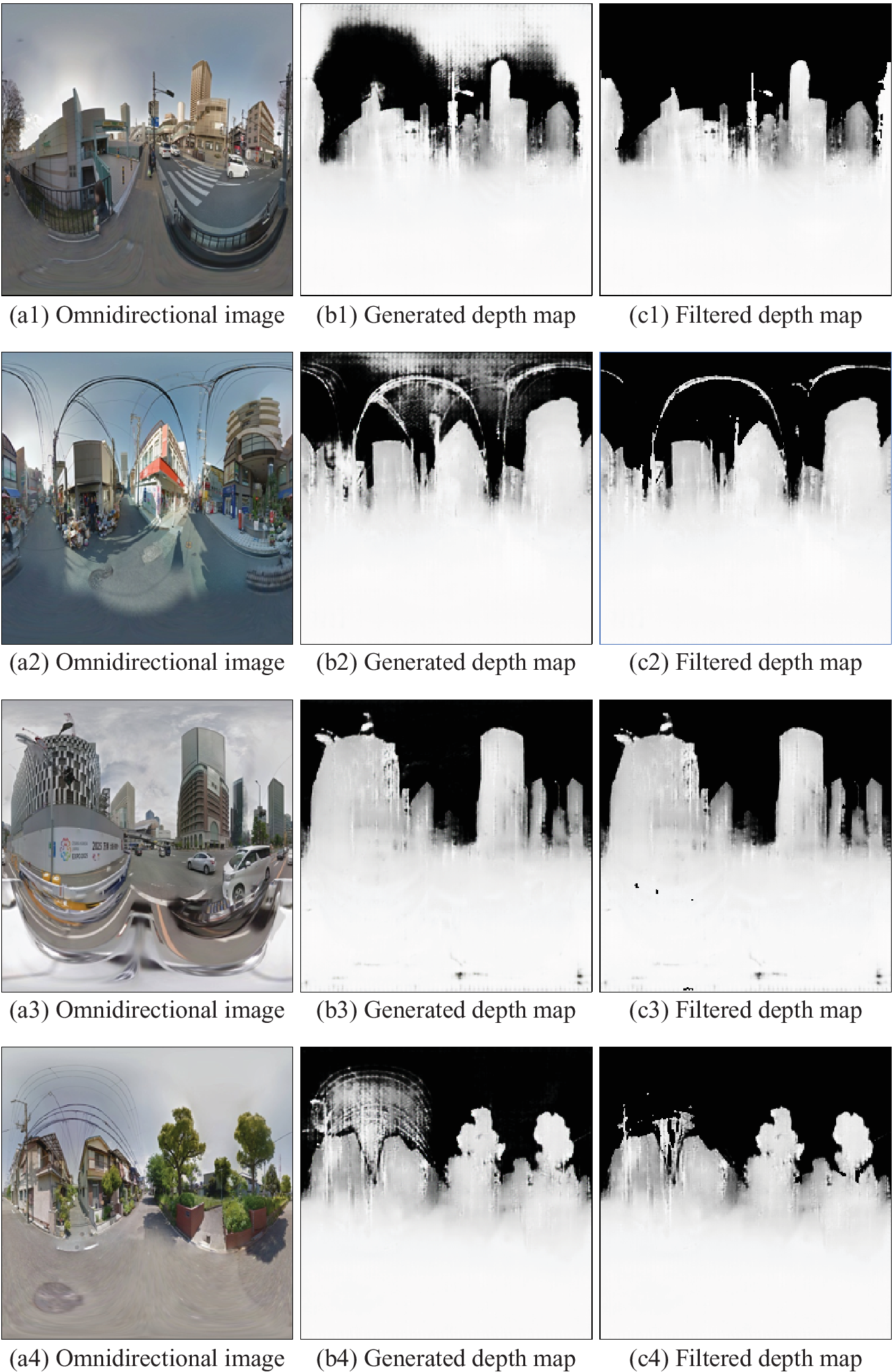
Figure 18. Example of depth maps of GSV (©Google, 2020) generated by M2c and their filtered depth maps.
3.3. Result of the preference scoring experiment (Step 2.1)
The mean preference score of each GSV image from 10 participants was used as the original value of the class label of the classification model described in Step 2.1. Table 3 lists the basic statistics of the preference score for 100 GSV images. The median and mean scores are 2.4 and 2.45, respectively, and there was no location that gave full marks to all subjects. The mean standard deviation (Std) of the score between examinees is 0.74; thus, it is evident that examinees’ preferences varied.
Table 3. Basic statistics of preference score of 100 GSV images.
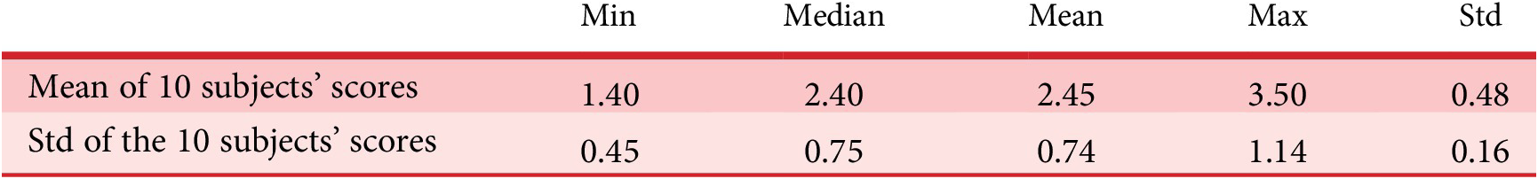
Figure 19 shows a histogram for each mean preference score of 100 GSV images. The frequency of the mean score is more around the median 2.4 while the number of cases in which the mean score is high or low is small, and there is a tendency of normal distribution although it is uneven. As described in Step 2.3, this distribution seems to be one of the reasons why predicted scores by a regression model tended to gather around the mean score in the preliminary experiment.
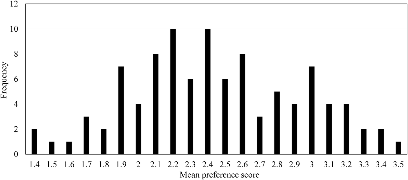
Figure 19. Histogram for each mean preference score of 100 GSV images.
Examples of images of places that received good, moderate and poor preference scores from all participants are shown in Figure 20. The images that received good preference score indicate that the subjects felt that the buildings in the images are not considered oppressive and that there is significant greenery and blue sky. On the other hand, in images that received poor preference score, houses and asphalt roads are evident.

Figure 20. Examples from GSV (©Google, 2020) preference scoring experiment in Osaka. The values are the mean/std of every 10 subjects’ scores.
3.4. Result of classification model (Step 2.3)
We think that it is more natural for a person to answer the preference scoring of the cityscape in four grades rather than to simply answer in two grades, that is, good or bad. On the other hand, in the classification problem, if the size of the data for each class is unbalanced, appropriate learning becomes difficult. The results of 10 evaluators were averaged for each image of GSV. When the mean preference scores of GSV were classified into four classes with the class boundary values as for example {1.5, 2.5, 3.5}, the corresponding number of cases of each class were 2, 52, 45 and 1 in ascending order from the class Bad, and most sites became moderately bad or moderately good. Since there is such unbalance in the number of each class, the problem was simplified to the two-class classification one.
According to Table 3, the median and mean preference scores are 2.4 and 2.45, respectively. From Figure 19, it can be seen that the distribution is spread in a form close to the right and left equally, with the median and mean values as the peak. Therefore, images with values greater than or equal to 2.5 or less were labelled Good or Bad, respectively. As a result, of 100 GSV images, 46 images have Good label and the remaining 54 images have Bad label. The image of GSV can be divided into two classes so that it is not perfectly uniform but not extremely imbalanced.
Then, 100 GSV images were divided into 80 images for learning, 10 images for validation and remaining 10 images for testing, so that the ratio of the number of each class was as uniform as possible in each data set, and fivefold cross validation datasets were constructed. In addition, in these five datasets, the roles of validation and testing were switched, and finally 10-fold cross-validation was performed. In each validation, the validation data were applied for each learning epoch, and the model of the epoch in which the loss value was minimum was used as the best model and the best model was applied to the test data, as well as the accuracy evaluation of the preference prediction was carried out. Since the classification performance is difficult to understand by the value of the loss function used in the learning, the final accuracy evaluation was carried out using the F1 score. The F1 score is the accuracy evaluation index for classification models considering the trade-off between precision and recall, and it shows that the classification performance is high as the value is close to 1, as well as the classification performance is low as it is close to 0. In the case of two-class classification problem, the F1 score in the case of random classification becomes 0.5. Therefore, an F1 score greater than 0.5 at the minimum is not an appropriate classification model.
Data augmentation was performed on 100 GSV images that are too small number for learning a CNN by the following procedure. To begin with, the images that were inverted right and left for the original image were generated. Then, these images, including the original ones, were made into images of the effect of rotating the camera by 18 degrees on the vertical axis. An omnidirectional image was saved in rectangular form as an equirectangular projection. Each image was divided into 20 equal parts in the vertical direction, and the left-end section of the image was moved to the right-end section for emulating camera rotation. As a result, 20 × 2 = 40 images, including the original, were generated for each GSV image. Therefore, learning, validation and training images were 40 × 80 = 3200, 40 × 10 = 400 and 40 × 10 = 400, respectively, and totally we have 4000 RGB and RGBD images.
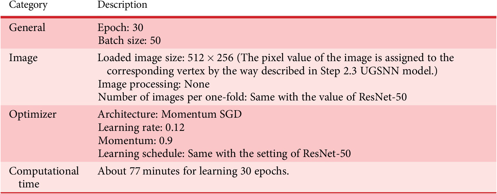
PyTorch was used as the framework to implement the learning task. The hyperparameters of ResNet-50 were as follows: number of epochs, 30; optimization method, Momentum SGD; moment, 0.9; learning rate, 0.05 (1–10 epochs), 0.025 (11–20 epochs) and 0.0125 (21–30 epochs); batch size, 200. Among the hyperparameters of UGSCNN, those which are different from those of ResNet-50 are as follows: learning rate, 0.12 (1–10 epochs), 0.06 (11–20 epochs) and 0.03 (21–30 epochs); batch size, 50. These learning settings of ResNet-50 and UGSCNN are summarized in Tables A2 and A3 in Appendix, respectively.
Figures 21 and 22 show the convergence process of the loss value in the learning and validation data of the RGBD images by ResNet-50 and UGSCNN, respectively. Although the learning data converge in about 20 epochs, the loss of the validation data inverts from about 10–15 epochs.
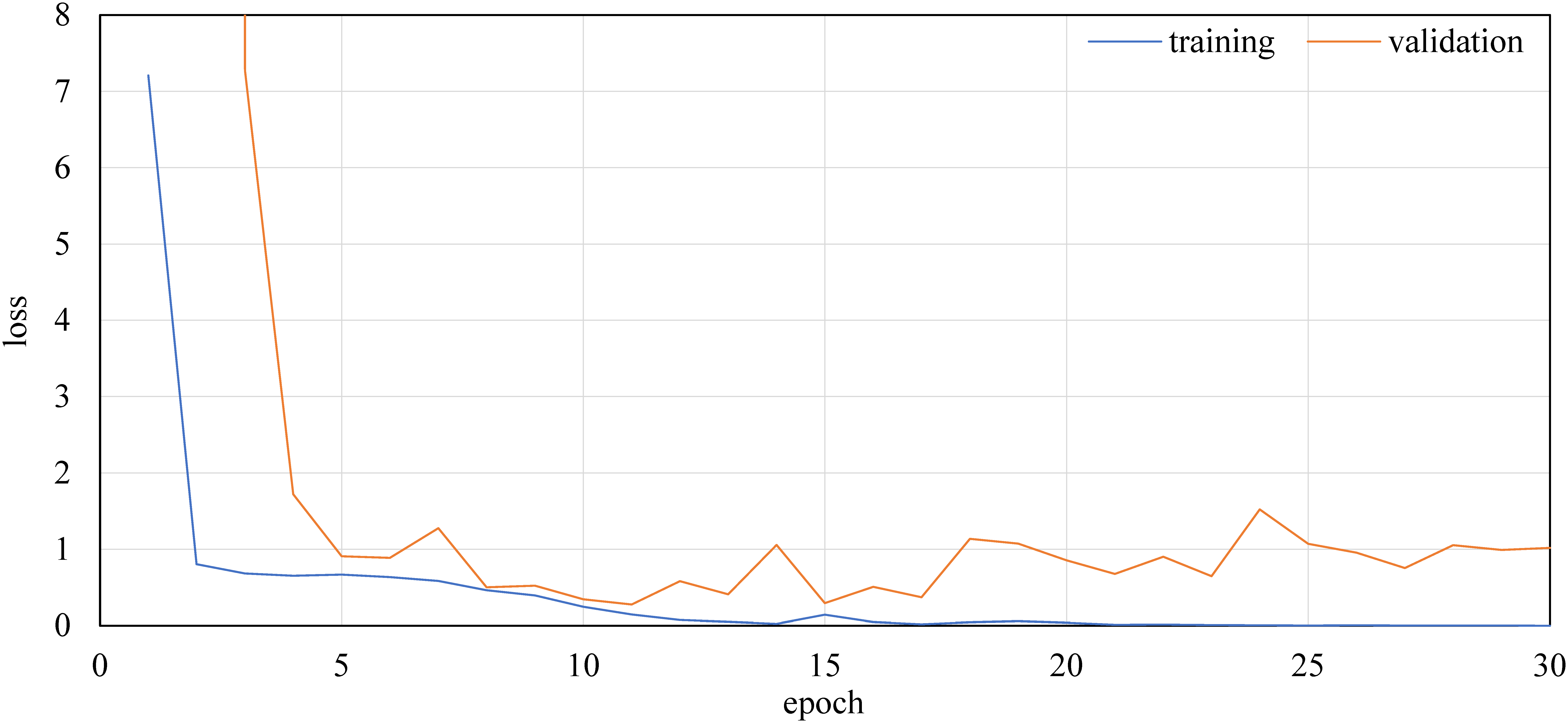
Figure 21. Example of the convergence process of loss functions of ResNet-50 with RGBD.
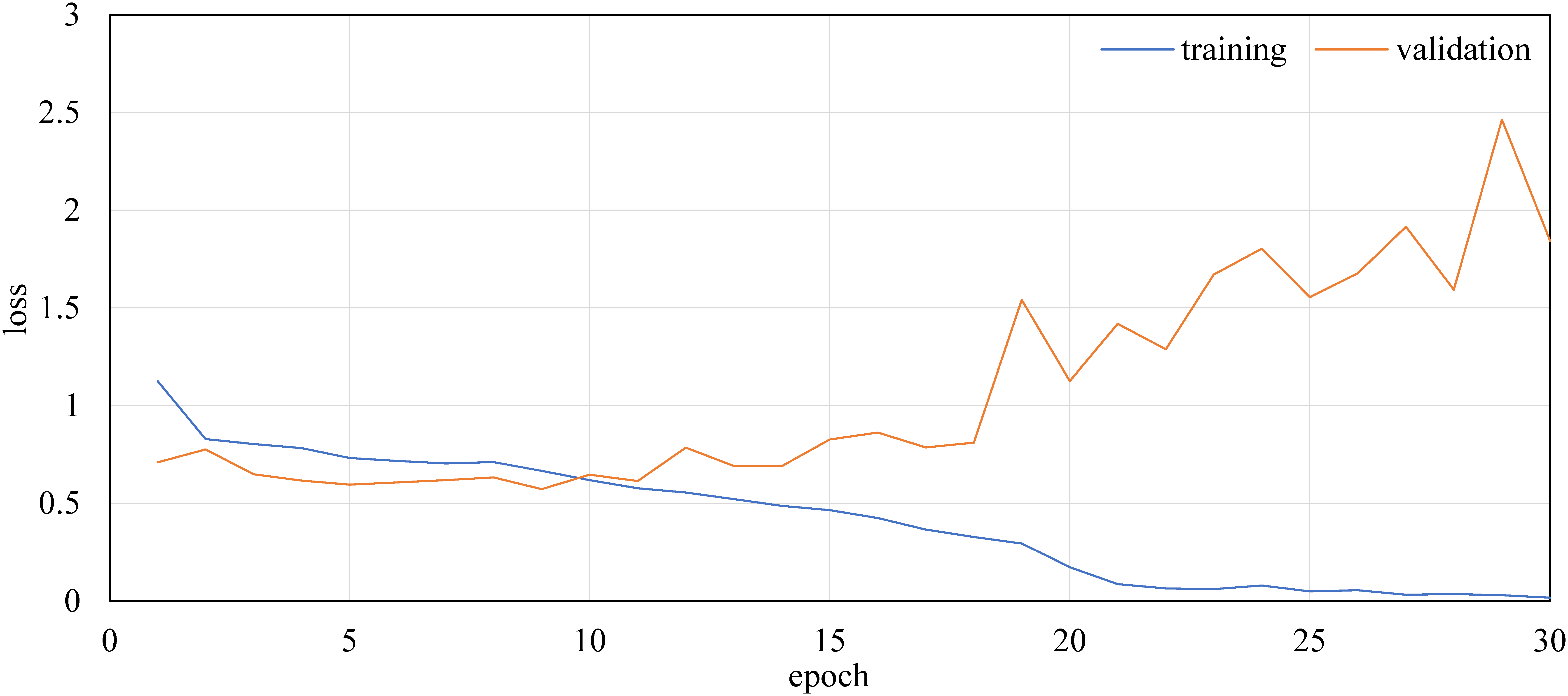
Figure 22. Example of the convergence process of loss functions of UGSCNN with RGBD.
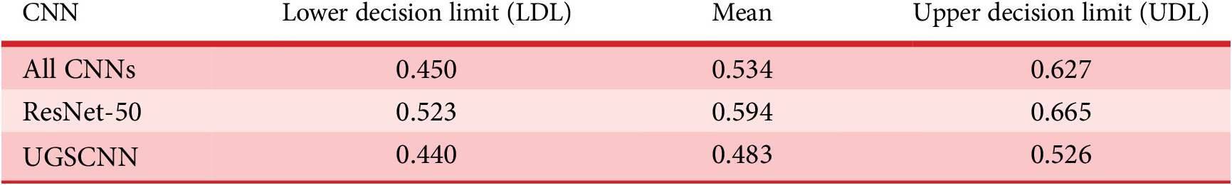
Figure 23 shows the distribution of F1 scores in the test data of each CNN by 10-fold cross validation. Table 4 lists the basic statistics of their F1 scores. Table 5 lists the decision limits of the analysis of means (Nelson, Wludyka, & Copeland, Reference Nelson, Wludyka and Copeland1987) for all CNNs and each type of CNNs. ResNet-50 is more accurate than UGSCNN. When all models are compared, the mean value of ResNet-50 with RGBD is superior to other models, and there is a statistically significant difference. On the other hand, in each type of CNNs while the mean and median values of the models trained by RGBD are higher, there are no significant differences statistically.
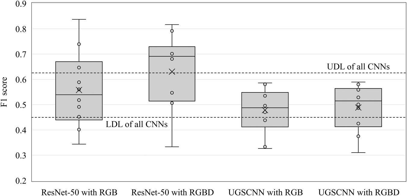
Figure 23. Distribution of F1 score of 10-fold cross validation for each CNN, X denotes mean.
Table 4. Descriptive statistics of F1 score of 10-fold cross validation for each CNN.
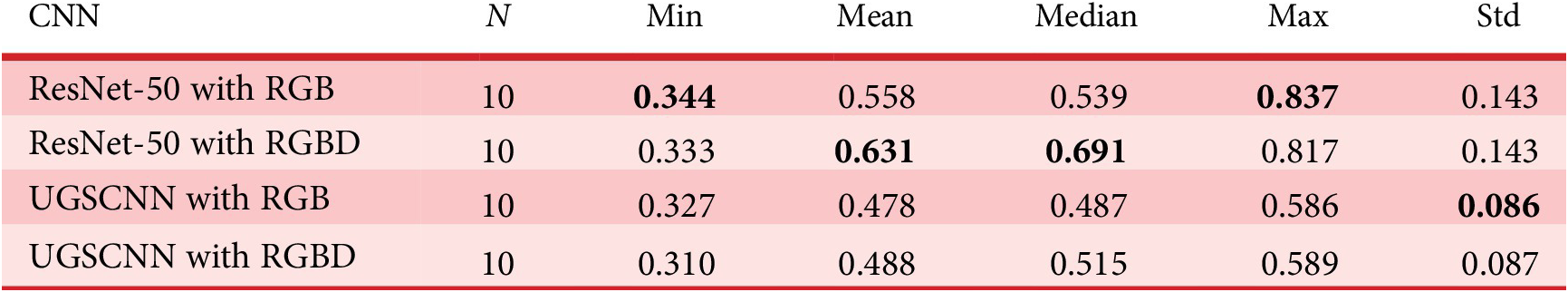
Table 5. Decision limit of analysis of means of F1 score for sets of CNNs, significance level = 0.05.
From the above results, it was shown that the classification accuracy of the CNN for usual rectangular image was higher than that of spherical CNN for prediction problem of spatial preference scoring of GSV. And, it is also concluded that the addition of depth maps to this problem may contribute to the improvement in the classification accuracy, but, at present, the effect of statistically significant difference could not be obtained.
4. Discussion
In this study, we demonstrated that depth maps are useful to evaluate street-level spatial images. In the following, we consider potential directions for future research.
4.1. Quality of the generated depth maps
In this study, the accuracy evaluation was carried out on the depth maps of CG generated with pix2pix by cross validation. The mean error of the depth for each pixel was about 2 m (= 5 pixel values) and it was visually acceptable to roughly grasp the depth of the cityscape.
It is important to confirm how much the error of the generated depth maps changes by the distance when considering the practicability and improvement policy of the model. Then, using the best M2c model used in the depth map generation of GSV, the absolute values of the error of pixel unit between generated depth maps and correct images for the test images of M3c were obtained. Next, the mean value and the standard deviation of the error were visualized for each distance in pixel value units (see Figure 24). The dotted graphs show the range of absolute error ± standard deviation. The error is small when the distance from the shooting point is close or far but the error becomes large as about 60 pixel value in the vicinity of 200 pixel value where the distance is a little far, and the error becomes unbalanced by the distance. The yellow area of the graph shows the logarithm of the number of pixels per distance. There are very many pixels that are close or far and few pixels whose distance is around 175 pixel value. It is considered that the difference of this number causes the unbalance of the error by the distance. The loss function of pix2pix has a term,
 $ {\mathcal{L}}_{L1}(G) $
, which minimizes the error between the correct image and the generated image. In order to eliminate unbalance of error due to distance, it is considered to modify
$ {\mathcal{L}}_{L1}(G) $
, which minimizes the error between the correct image and the generated image. In order to eliminate unbalance of error due to distance, it is considered to modify
 $ {\mathcal{L}}_{L1}(G) $
so that it is weighted considering the number of pixels due to distance.
$ {\mathcal{L}}_{L1}(G) $
so that it is weighted considering the number of pixels due to distance.
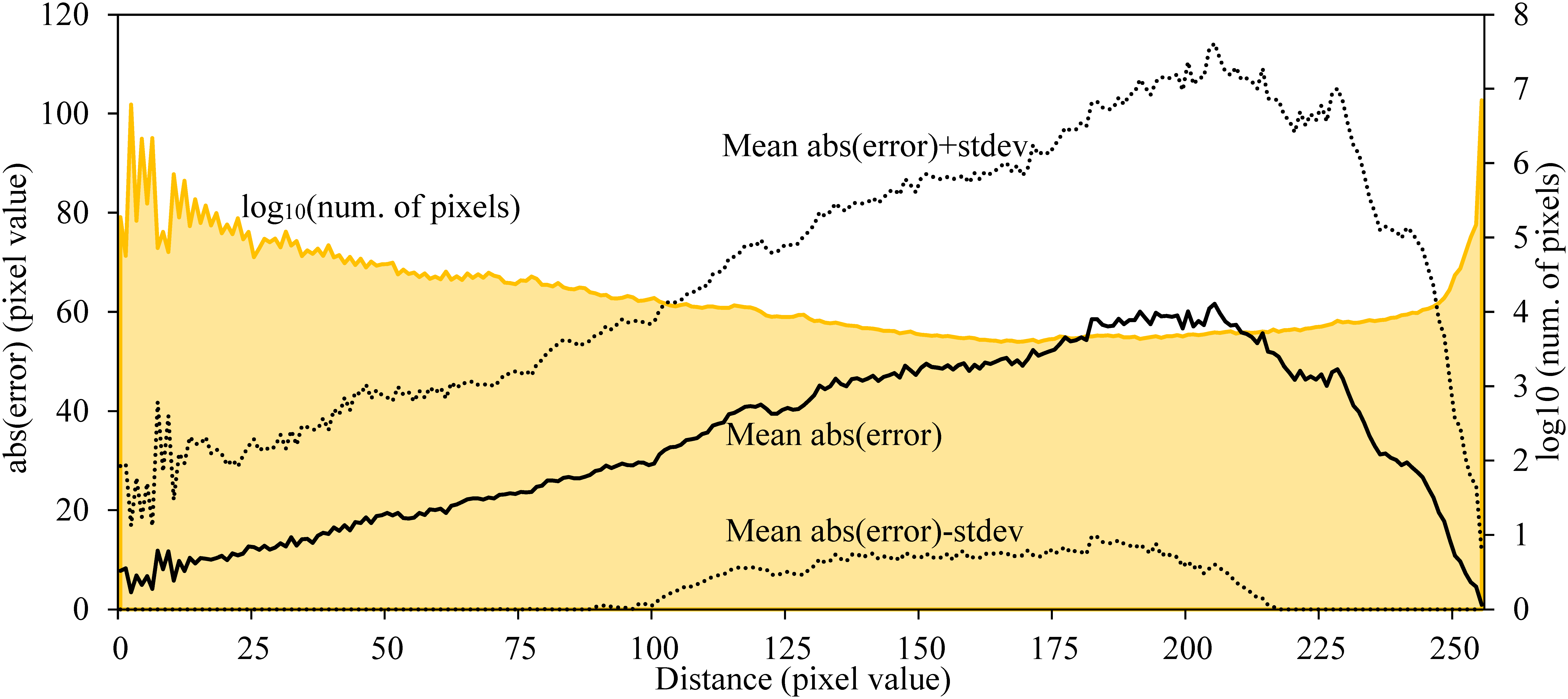
Figure 24. Mean absolute error of pixel unit between generated depth maps and correct images and number of pixels for each distance.
In Table 2, RMSE of Shibuya model (M1*) was less than that of local cities (M2*). When the mean depth of the images of each 500 observation points in Shibuya and local city was calculated, it was about 77.6 pixel unit in Shibuya and 89.0 in the local city, and the openness of the space was better in the local city. As shown here, except for the sky part, the farther the pixel value is, the larger the estimation error tends to be. Therefore, it is considered that the value of RMSE is smaller in the Shibuya model where the pixels are relatively close.
On the other hand, since there was no ground-truth dataset to verify the depth map generated from the GSV images, the model that generated the most appropriate depth maps was chosen from nine pix2pix models subjectively by visual judgment. The noise in the sky part was almost eliminated by the SS. As for the depth of buildings, etc., the image is subjectively reasonable to some extent, but the accuracy is worse than that of CG images. When these depth maps were incorporated into the preference prediction model, the accuracy of the model was slightly improved, so it is not likely to be at least a random depth map. However, it cannot be said that the accuracy of the preference prediction model is high because the mean F1 score of the cross verification is 0.63 at the maximum. Thus, for example, if the model is used for site recommendations, false-positive results will be noticeable. In the future, it will be necessary to fill the gap of the accuracy of the depth map of CG and GSV by utilizing the technology of domain adaptation (Wang & Den Wang & Deng, Reference Wang and Deng2018), etc.
In fact, there exist depth maps in GSV (nøcomputer, 2017) but it is difficult to evaluate the depth map using it since there are no depth information (see Figure 25), or even if there are only a partial depth information of the short distance part and it is very simplified. To quantitatively evaluate the depth of the space, it is necessary to measure the space using an outdoor laser scanner. However, the laser range is only a few hundred metres at the most; therefore, the measurement distance may be insufficient to this study, which deals with outdoor visibility. Recently, photogrammetry technology has been developed and Google Earth offers detailed 3D urban models of large cities, such as London (Google, n.d.). Depth maps should be verified quantitatively, considering the effectiveness of such related technology and the availability of data.
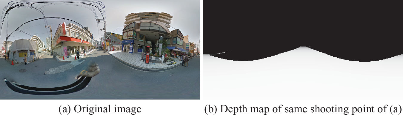
Figure 25. Example of a depth map of GSV (©Google, 2020).
4.2. Potential of SS in spatial preference scoring
We extracted the part of the image classified as sky using an existing SS method and removed the noise of the corresponding part of each depth map. However, verification is necessary because the image data obtained via SS may be related to human spatial preference, such as those studied in this paper. It is possible that, to some extent, our preference scoring experiment results suggest that the openness of the space and the abundance of green are related to human spatial preference. It is necessary to clarify what type of spatial information image is related to such spatial preference by constructing a preference prediction model that uses SS images.
4.3. Possibility of spherical CNNs
In fact, the preliminary experiment had been carried out not only with pix2pix but also with OminiDepth corresponding to an omnidirectional image for generating the depth map of GSV. However, OmniDepth had generated blank images. That is, although pix2pix has some robustness for images of different domains, OmniDepth has no robustness. The possible reason for this is that pix2pix uses the instance normalization, which is used in style conversion of CNNs, and has a complicated evaluation structure that does not simply minimize the error with the ground truth image. Combining pix2pix’s learning strategy with the convolution method of OmniDepth may enable more accurate omnidirectional depth map generation.
In addition, the UGSCNN, used as the preference prediction model of GSV, predicts with low accuracy. UGSCNN outperforms other well-known spherical CNNs in several benchmarks for omnidirectional images but it was not effective for our data. For this reason, it is considered that the structure of the UGSCNN has not been sufficiently examined yet. At present, the structure of UGSCNN was designed by referring to an implementation example for image classification but it is necessary to find a structure more suitable for our dataset by trial and error. In addition, since the research of CNNs for general rectangular images is greatly advanced in comparison with that of spherical CNNs, it is considered that the performance of ResNet was more easily obtained even if it was applied to omnidirectional images. Finally, street space is generally composed of ground at the foot and sky at the top. Therefore, perfect sphericity may not always be necessary to model it and an approximate method, such as panoramic projection, may be enough. This raises the question of how well geometrically sophisticated spatial analysis techniques, such as spherical CNNs and 3D isovist, are effective, for what scale and type of space. Further research is necessary.
4.4. Need for problem setting in which spatial attributes are more dominant
As described in Section 2.2, this time, the preference scoring experiment of GSV was carried out in accordance with individual sensibilities without intentionally giving uniform criterion. Therefore, there were some examples in which it was guessed that the image was evaluated by the attribute except for the space, for example, to prefer the image containing the blue sky. This may be one reason why the prediction accuracy of GSV was not greatly improved even with the estimated depth maps. Therefore, some guidance may be better to verify the effectiveness of depth map. In relation to this issue, most of the images of GSV used this time were taken from the road by the automobile and the diversity of the near view might be lacking in the sense of spatial composition. The GSV includes images of narrow alleys, which cannot be shot by automobiles. Especially in cityscapes in Japan, such narrow spaces are likely to be preferred by pedestrians. Based on the above points, it is necessary to improve the problem setting so that the spatial attribute becomes a more important factor.
4.5. Need for larger dataset
In this study, 20 subjects learned their preferences for GSV images on CNNs at a total of 100 sites. Although, the number of images was increased from 100 to 4000 for learning, validation and test by the data augmentation but the classification accuracy was not high. It seems to be not sufficient size as a data set of the deep learning model of two-class classification. Since it is not easy to increase the data of preference experiments, it may be necessary to devise an online service, such as Scenic-Or-Not to create a large data set. On the other hand, objective and large-scale data related to space, such as land prices and real estate rents are already available. Although it is another problem setting, it may be necessary to examine the use of such dataset for the verification of our proposed method.
5. Conclusion
In this study, we developed a method for generating omnidirectional depth maps from the corresponding omnidirectional images of cityscapes by learning each pair of omnidirectional images and depth maps created by CG using pix2pix. Models trained with different series of images shot under different site and sky conditions were applied to GSV images to generate depth maps. The validity of the generated depth maps was then evaluated quantitatively and visually. Then, we conducted experiments to score cityscape images of GSV using multiple participants. We constructed models that predict the preference class of these images with and without the depth maps using the classification method with CNNs for general rectangular images and omnidirectional images. The results demonstrated the extent to which the generalization performance of the preference prediction model of the cityscape changes depending on the type of CNNs and the presence or absence of depth maps. As a result, we have the following conclusions.
The depth of CG images was quantitatively evaluated and the mean error is about 2 m per image. In the sense of street-scale spatial analysis, such an error is acceptable. However, when the error of the pixel was examined according to the distance, the error of the pixels in the slight distant was relatively large.
On the other hand, on the generated depth maps of GSV, which is a real image, visual evaluation was carried out, and it was confirmed that the accuracy was inferior compared with CG, even if the noise of sky part was ignored. However, the qualitative tendency of the space, such as near and far of the object was able to be grasped.
In the preference prediction problem of GSV images, the best classification accuracy was achieved by ResNet-50 for the general rectangular image with RGBD images, and the accuracy of the UGSCNN for omnidirectional images was bad in either images. Although the effect of the depth map was not statistically significant, the result implies the necessity of considering the depth maps for modelling visual preference of space. Since the absolute accuracy of the image classification model itself is not high, it is necessary to increase the data and to find the problem of the space where the geometrical feature is more important, such as complex indoor space. These results support the findings of a previous study (Takizawa & Furuta, Reference Takizawa and Furuta2017). That is, an automatic preference prediction model for street space should consider the colour, texture and geometric properties of the space.
The points to be improved in the future are as follows.
We improved the accuracy of depth maps by expanding pix2pix for omnidirectional images, considering the unbalance of estimated depth error by distance and improving the estimation accuracy between CG and real images by domain adaptation.
Since the classification accuracy of CNNs for predicting preference of GSV images, especially that of the spherical CNN, was low, the model should be improved by grasping which part of the image CNN pays attention to by techniques such as GradCAM (Selvaraju Selvaraju et al., Reference Selvaraju, Cogswell, Das, Vedantam, Parikh and Batra2017), by dimension reduction technique such as principal component analysis, etc. In this connection, what kind of feature of the space is deeply related to recognition and preference should be grasped by novel approach different from the conventional isovist analysis techniques, and the proposed model should be improved to the spatial analysis model with higher explanatory power.
We should compare the result with other machine learning models with conventional image features, such as scale-invariant feature transform (SIFT; Lowe, Reference Lowe2004) and/or the images of SS.
It is necessary to find the network structure of the CNN that matches this problem more.
It is necessary to improve the problem setting of the preference scoring experiment of space so that the spatial attribute becomes a more important factor.
Financial Support
This study is partially supported by Grant-in-Aid for Scientific Research (A) (16H01707) and (C) (20 K04872).
Supplementary Materials
To view supplementary material for this article, please visit http://dx.doi.org/10.1017/dsj.2020.27.
Appendices
About learning settings of CNNs
Learning settings of our deep learning S models for learning are listed in Tables A1–A3.
Table A1. Learning settings of the pix2pix model
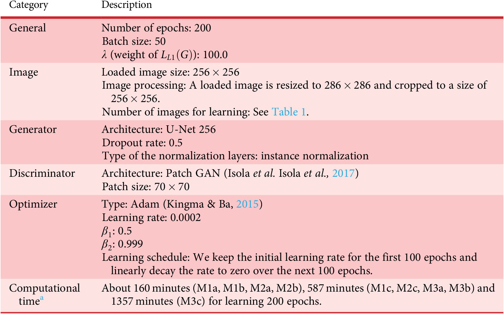
a CPU, Intel Core i9 7940×; memory DDR4 2400 16GB × 8 = 128GB, GPU, Nvidia TITAN RTX (24GB Memory) × 2; Windows 10 Professional, CUDA 10.1, cuDNN 7.6.5, PyTorch 1.4.0.
Table A2. Learning settings of ResNet-50 model
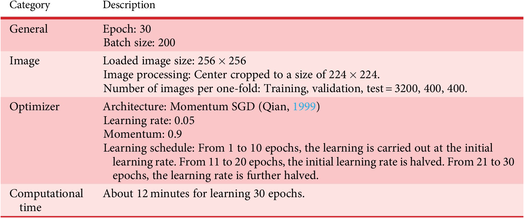
Table A3. Learning settings of UGSCNN model
About DeepLab v3+
Many semantic segmentation models are based on the encoder-decoder structure (Figure A1a) as well as pix2pix. This structure can obtain sharp object boundaries at high speed, but hierarchical information is easily lost at the encoding stage. The Spatial pyramid pooling model (Figure A1b) is suitable to hold hierarchical information, but, conversely, the boundary part of the generated image tends to be blurred. DeepLab v3+ is a segmentation model that integrates the advantages of both methods (Figure A1c). In addition, DeepLab v3+ features convolution at high speed with explicit control of resolution by using an atrous depthwise convolution, which can parametrically change adjacent pixels through the channel direction, instead of the usual convolution (Figure A2).
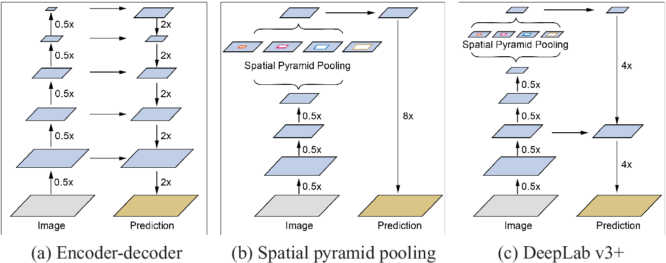
Figure A1. Structure of semantic segmentation models.
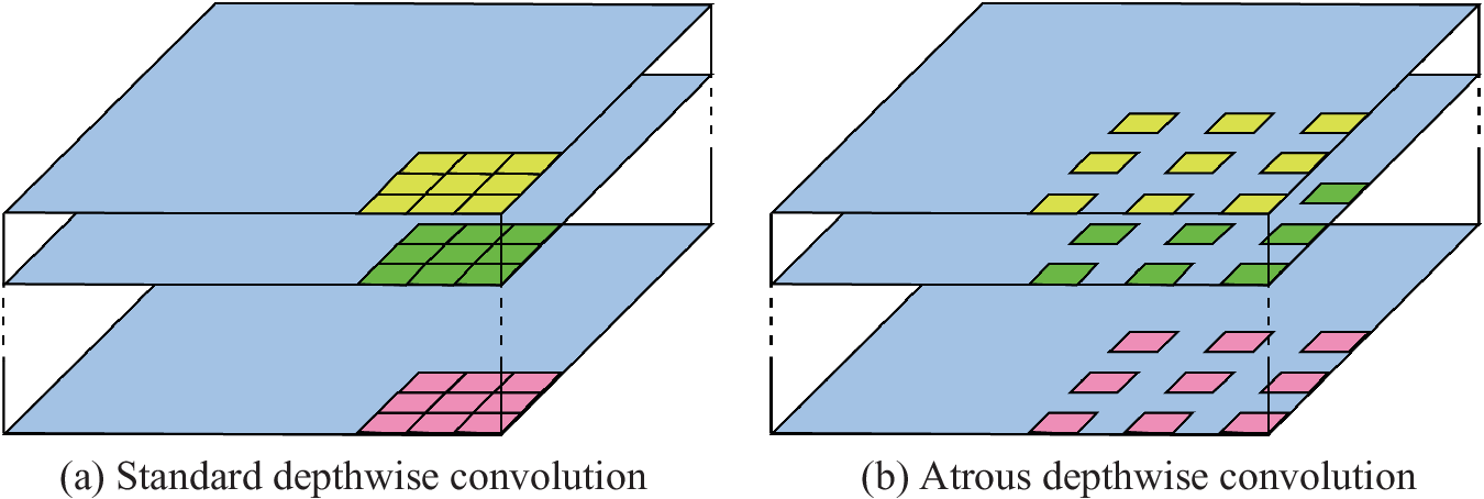
Figure A2. Type of depthwise convolution.


 Open access