


Impact Statement
Tracking greenhouse gas (GHG) emissions globally is a challenge of increasing importance to enable targets for emissions reduction and measure progress toward them. Quantifying road transportation emissions is particularly difficult due to the distributed nature and large number of sources involved. Our approach is a scalable and accurate method to estimate road activity and GHG emissions for individual road segments in large urban cities around the world, which can lead to a better understanding of where to focus emission mitigation efforts.
1. Introduction
Transportation contributed 27% of anthropogenic greenhouse gas (GHG) emissions in the U.S. for 2020, higher than any other sector, and 12.6% of all global GHG emissions in 2019 (Agency UEP, 2022; World Resource Institute, 2022). The primary source of transportation sector emissions is on-road vehicles, accounting for approximately 74% of global transportation emissions in 2018 (International Energy Agency (IEA), 2022). Quantifying the distribution of on-road transportation emissions and creating timely emissions inventories are vital to identify trends, track mitigation efforts, and inform policy decisions.
Previous efforts have developed detailed bottom-up on-road emission inventories for the U.S. (Gately et al., Reference Gately, Hutyra and Wing2015; Gurney et al., Reference Gurney, Liang, Patarasuk, Song, Huang and Roest2020), but do not easily extend globally due to the reliance on vehicle traffic and road data that is not always readily available. EDGAR (Janssens-Maenhout et al., Reference Janssens-Maenhout, Crippa, Guizzardi, Muntean, Schaaf, Dentener, Bergamaschi, Pagliari, Olivier, Peters, van Aardenne, Monni, Doering, Roxana Petrescu, Solazzo and Oreggioni2017) provides a global inventory for transportation that uses road density as a proxy to spatially distribute emissions. However, some emission estimates for urban centers in EDGAR deviated from other bottom-up inventories (Gately et al., Reference Gately, Hutyra and Wing2015) by 500%, indicating that road density is not a sufficient proxy for global high-resolution inventories. Carbon Monitor (Liu et al., Reference Liu, Ciais, Deng, Davis, Zheng, Wang, Cui, Zhu, Dou, Ke, Sun, Guo, Zhong, Boucher, Bréon, Lu, Guo, Xue, Boucher and Chevallier2020) is a global emissions inventory that utilizes a variety of activity data to estimate daily GHG emissions, however, the reliance on proprietary traffic data in the ground transportation sector limits the ability to extend to locations where this data is not available. Other methods have used machine learning (ML) to directly predict emissions, but their ability to generalize globally is unclear (Mukherjee et al., Reference Mukherjee, Rollend, Christie, Hadzic, Matson, Saksena and Hughes2021; Scheibenreif et al., Reference Scheibenreif, Mommert and Borth2021).
We propose an emissions estimation method that is globally accurate while using openly available input data. It combines remote sensing, geospatial data, and ML with traditional, “bottom-up” emissions inventories that directly incorporate region-specific vehicle fleet mix, fuel efficiency, and other emissions factors (EF) data. This approach, illustrated in Figure 1, is composed of two independent ML models to predict road transportation activity and an EF pipeline that translates activity to emissions in a localized fashion. The results from these models are ensembled to provide a single output. Splitting the ML and EF parts affords continuous improvement as newer data become available. Our contribution is a method that uses ML-predicted road activity along with region-specific emissions factors data to create up-to-date and global on-road GHG emissions estimates.

Figure 1. System architecture for our hybrid emissions estimation model.
Specifically, we use ML to predict activity in the form of the average annual daily traffic (AADT), or the number of vehicles traveling on a given road segment per day, on average, over an entire year. Separately, we can estimate the EF based on city- or region-specific vehicle-related data. We then combine the EF, the AADT, and segment information to estimate emissions for each road segment. Summing the emissions from all road segments provides an estimate of annual GHG emissions for a city.
This paper is organized as follows. Sections 2–4 introduce the source data, the ML methods used to predict road activity, and the transformation from activity to emissions. Section 5 provides the results of the ML models, which we discuss in detail in Section 6. Finally, Section 7 discusses future work and summarizes the results in a conclusion.
2. Data
We formulate the road activity prediction task as a regression problem. We train models to predict AADT, or the number of vehicles traveling on a given road segment per day, on average over an entire year. In our prediction task, we used two different ML models: a convolutional neural network (CNN) as well as a graph neural network (GNN). For the CNN model, we used two sources of input data: RGB satellite imagery as well as rasterized road network data. The GNN model used road network data to generate information for nodes and edges of the input graph. In both ML models, we use ground truth data from the U.S. Highway Performance Monitoring System AADT data set from 2017 (US Federal Highway Administration, 2017). This AADT data is recorded using roadside devices and is typically only recorded on major highways and arterial (collector) roads. Models trained in the U.S. are then run over both U.S. and global cities for evaluation.
In this section, we describe the source data used for training the ML models, the reasoning behind choosing 500 global cities, and the data sources for emissions factors used to turn AADT activity into city-wide estimates of GHG emissions.
2.1. Cities selection
To date, our hybrid emissions estimation pipeline has been run on a prioritized set of 500 global cities. To prioritize the cities, we utilized the European Union Joint Research Center Global Human Settlement Layer Urban Centers Database (GHSL-UCDB) dataset (Florczyk et al., Reference Florczyk, Corbane, Schiavina, Pesaresi, Maffenini, Melchiorri, Politis, Sabo, Freire, Ehrlich, Kemper, Tommasi, Airaghi and Zanchetta2019) for a globally consistent representation of city extent. This database contains the geographic bounds and other metadata for approximately 13,000 cities worldwide and utilizes a definition of city/urban center based on population density and built-up area. Specifically, an urban center was defined as “the spatially generalized high-density clusters of contiguous grid cells of 1 km2 with a density of at least 1500 inhabitants per km2 of land surface or at least 50% built-up surface share per km2 of land surface, and a minimum population of 50,000” (Florczyk et al., Reference Florczyk, Corbane, Schiavina, Pesaresi, Maffenini, Melchiorri, Politis, Sabo, Freire, Ehrlich, Kemper, Tommasi, Airaghi and Zanchetta2019). Due to this definition, city geometries in UCDB often have significantly different shapes and sizes as compared to official administrative bounds, for example, from OpenStreetMap (OSM) (Haklay and Weber, Reference Haklay and Weber2008) or Global Administrative Areas (GADM) (Global Administrative Areas, 2022). We note that these differences are likely a main cause of discrepancies between our emissions estimates and other inventories.
UCDB spatially combines urban centers with a variety of metadata related to geography, socioeconomic, environment, disaster risk, and sustainable development goals. This metadata includes EDGAR V5.0 (Janssens-Maenhout et al., Reference Janssens-Maenhout, Crippa, Guizzardi, Muntean, Schaaf, Dentener, Bergamaschi, Pagliari, Olivier, Peters, van Aardenne, Monni, Doering, Roxana Petrescu, Solazzo and Oreggioni2017) emissions estimates within urban center bounds for 1975, 1990, 2000, and 2015. We used the 2015 transport sector total CO2 emissions from nonshort-cycle organic fuels (fossil fuels, CO2_excl_short-cycle_org_C in EDGAR) to sort and select the largest 500 cities for this work. The distribution of the selected cities across continents is shown below in Table 1.
Table 1. Regional distribution of the 500 global cities selected for emissions estimation

Additional datasets from the GHSL effort include the GHSL BUILT-S (Pesaresi and Politis, Reference Pesaresi and Politis2022) and GHSL POP (Schiavina et al., Reference Schiavina, Freire and MacManus2022). These were used on a trial basis when testing additional model features (see Section 3.3). The GHSL BUILT-S dataset is a global raster dataset that provides a measure of how much of the Earth surface is built-up, measured in square meters per grid cell. The GHSL POP dataset is a global raster dataset that provides population density estimates per grid cell.
2.2. OpenStreetMap
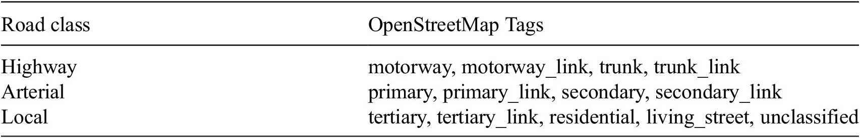
OSM (Haklay and Weber, Reference Haklay and Weber2008) road network data is used as an input to our models and for associating predicted AADT values with their corresponding physical road segment. While OSM can contain inconsistencies and is not complete, its open access and global availability make it suitable for this work. In order to standardize terminology across the CNN and GNN models, we reduced the number of OSM road types to three. The current supported road types are highway, arterial, and local, which were chosen to align with other similar emissions inventories and traffic-related databases; the mapping between these road types and their respective OSM tags are shown in Table 2. Road type categorization is important in the emissions factor calculation for a given road segment as other emissions factors variables, including vehicle fleet mix and fuel efficiency, can vary significantly across different types of roads.
Table 2. Mapping of the three road types used in our emissions calculation to their corresponding OSM tags
2.3. Training data
In both ML models, we use ground truth data from the U.S. Highway Performance Monitoring System AADT data set from 2017 (US Federal Highway Administration, 2017) for a set of 14 cities in the US. This AADT data is recorded using roadside devices and is typically only recorded on major highways and arterial (collector) roads. Specifically, AADT data is sparse, making up single-digit percentages of the road network.
Using this as the only training data set imposes several possible biases on our estimates. First, global traffic patterns are not likely to reflect those in the US. Additionally, the lack of full coverage may bias our ML models to lower prediction values. As we argue in Section 6.2, however, our predicted values for total emissions correlate well with other datasets. For more details on these comparisons, see Section 6.
2.4. Satellite data
We use two different sources for RGB Satellite imagery: Sentinel-2 and Planet Labs.
The European Space Agency’s (ESA) Sentinel-2 mission comprises two satellites- Sentinel-2A, launched in 2015, and Sentinel-2B, launched in 2017 (Main-Knorn et al., Reference Main-Knorn, Pflug, Louis, Debaecker, Müller-Wilm and Gascon2017). Each Sentinel-2 satellite has a 10-day revisit time with a 5-day combined revisit. Both satellites are equipped with a multispectral (MSI) instrument which provides 13 spectral band measurements, blue to shortwave infrared (SWIR) wavelengths (442–2202 nm) reflected radiance. We used the Sentinel-2 Level-2A product at 10 m × 10 m resolution, using bands 4 (red), 3 (green), and 2 (blue) (Drusch et al., Reference Drusch, Del Bello, Carlier, Colin, Fernandez, Gascon, Hoersch, Isola, Laberinti, Martimort, Meygret, Spoto, Sy, Marchese and Bargellini2012).
Planet Lab’s PlanetScope satellite constellation consists of approximately 130 individual satellites, called “Doves,” with the first launch of this constellation in 2014 (Planet Labs, 2022). Each PlanetScope satellite images the earth’s surface in the blue, green, red, and near-infrared (NIR) wavelengths (450–880 nm). We acquired PlanetScope (Planet Labs, 2022) approximately 3 m resolution monthly and quarterly mosaics over the various geographic extents of the cities we used for training, validation, and global inference.
2.5. Emissions factors
Transportation EFs are dependent on many variables, including (but not limited to) road category, vehicle mix, fuel type, and fuel efficiency. Data collection for each of these EF-related variables across 500 cities is a significant undertaking. The initial version of estimated emissions factors focused on collecting data at the country-level for the 86 countries in which the top 500 cities are located.
2.5.1. Vehicle fleet mix
Vehicle fleet mix refers to the distribution of total vehicles in a given country across various vehicle types. The supported vehicle types were: passenger cars, light duty trucks, single unit trucks, combination trucks, motorcycles, and buses. Country-specific vehicle fleet data was used for 36 countries, while a U.S. urban area average derived from U.S. Federal Highway Administration (FHWA) data (Highway Statistics, 2020) was used for the remaining 50 countries until further country-specific data sources were identified.
A full listing of the 36 countries with country-specific data and their respective sources is listed in Table 3. Due to differences in the vehicle type taxonomy across countries, vehicle types were manually recategorized to the supported vehicle types as well as possible. Vehicle fleet mix values are currently the same across all supported road types, but will be updated as sources of road type-specific data are identified.
Table 3. Listing of specific data sources used in estimated vehicle fleets in specific countries

2.5.2. Fuel type and efficiencies
Due to the fact that different fuel types have different emissions factors, it is important to know the relative mix of fuel types for each type of vehicle traveling on a given road segment. The types of supported fuels are gasoline, diesel, compressed natural gas (CNG), liquefied petroleum gas (LPG), plug-in hybrid, battery electric vehicle (BEV), and other fuels (e.g., biogas, ethanol). The primary source of this data is the Climate Action for Urban Sustainability (CURB) tool (World Bank Group, 2019), which provides a global database of fuel type mix by country. Future updates may include updated country or city-specific fuel type data.
CURB was also the primary source of fuel efficiency data for all 86 countries. CURB fuel efficiency values are reported in units of kilometers per liter and were extracted for all supported fuel and vehicle types described above. Fuel efficiencies were the same across all supported road types (highway, arterial, and local) in this release, but may be continuously updated as better country or city-specific datasets are located.
2.5.3. Vehicle GHG emissions factors
GHG emissions factors refer to how much of a given gas is emitted per unit of fuel burned and varies by fuel type. Our data focuses on carbon dioxide (CO2), nitrous oxide (N2O), and methane (CH4) emissions factors, using data from the U.S. Environmental Protection Agency (2022). For nitrous oxide and methane, the emissions factors for each gas were given in units of grams of each gas per mile driven. This was different from the data for carbon dioxide, which was given as grams per liter. To normalize all GHG emissions factors to “grams per liter,” we used fuel efficiency data (given in “liters per km”) to generate data for nitrous oxide and methane as grams per liter.
3. ML models
In this section, we describe each type of ML model separately as they can be analyzed independently although they use similar underlying training data. Analysis of the performance of each family of models is performed separately. However, the final emissions estimates come from an ensemble of two models as described in Section 4.
3.1. Metric definitions
The following metrics are used to analyze both predicted AADT and, below, city-level emissions from our CNN and GNN ML models. In each equation,
 $ n $
represents the number of roads or cities under consideration,
$ n $
represents the number of roads or cities under consideration,
 $ i $
represents the road or city index,
$ i $
represents the road or city index,
 $ P $
represents the predicted AADT or predicted emissions from our model, and
$ P $
represents the predicted AADT or predicted emissions from our model, and
 $ \mathrm{GT} $
represents the ground-truth AADT or emissions value.
$ \mathrm{GT} $
represents the ground-truth AADT or emissions value.
 $$ \mathrm{Mean}\ \mathrm{Error}:\hskip1em \frac{1}{n}\sum \limits_{i=1}^n\left({P}_i-{\mathrm{GT}}_i\right). $$
 $$ \mathrm{Root}\ \mathrm{Mean}\ \mathrm{Squared}\ \mathrm{Error}\;\left(\mathrm{RMSE}\right):\hskip1em \sqrt{\frac{1}{n}\sum \limits_{i=1}^n{\left({P}_i-{\mathrm{GT}}_i\right)}^2}. $$
 $$ \mathrm{Mean}\ \mathrm{Absolute}\ \mathrm{Percentage}\ \mathrm{Error}\;\left(\mathrm{MAPE}\right):\hskip1em \frac{100}{n}\sum \limits_{i=1}^n\frac{\mid {P}_i-{\mathrm{GT}}_i\mid }{{\mathrm{GT}}_i}. $$
 $$ \mathrm{Mean}\ \mathrm{Percentage}\ \mathrm{Error}\;\left(\mathrm{MPE}\right):\hskip1em \frac{100}{n}\sum \limits_{i=1}^n\frac{P_i-{\mathrm{GT}}_i}{{\mathrm{GT}}_i}. $$
Additionally, we use the scipy.stats implementation of Pearson’s
 $ \rho $
coefficient to calculate correlations (scipy.stats.pearsonr, n.d.).
$ \rho $
coefficient to calculate correlations (scipy.stats.pearsonr, n.d.).
Multiple metrics are used for analysis as they are each sensitive to different error sources, especially when considering how AADT and city emission values vary over several orders of magnitude. Mean Error and MPE are useful in evaluating bias in emissions and AADT prediction. RMSE will be most sensitive to large outliers. The relative error terms (MAPE and MPE) are very sensitive to errors in lower trafficked roads/emitting cities due to the division by
 $ {\mathrm{GT}}_i $
. In contrast, the other error terms (Mean Error, RMSE, and Pearson’s
$ {\mathrm{GT}}_i $
. In contrast, the other error terms (Mean Error, RMSE, and Pearson’s
 $ \rho $
) will be more influenced by errors on higher trafficked roads/emitting cities due to their larger scale.
$ \rho $
) will be more influenced by errors on higher trafficked roads/emitting cities due to their larger scale.
3.2. Convolutional neural networks
Architectures derived from semantic segmentation convolutional neural networks (CNNs) were trained to predict AADT, using visual RGB satellite imagery and road network data. Separate models were trained using the two sources of imagery. OSM data is rasterized for the corresponding extent of an input visual image, where each standardized road type (highway, secondary, local) is rasterized independently, and the resulting raster channels are concatenated together to form a three-channel image (see Table 2 for associated OSM tags for each road type). This image is combined with the visual satellite image to form a six-channel image that is fed to the CNN to predict AADT on a per-pixel basis. We primarily use MANet-based architectures (Fan et al., Reference Fan, Wang, Li and Wang2020) for our segmentation models, with EfficientNet (Tan and Le, Reference Tan and Le2019) backbones. The model architectures diverge from standard semantic segmentation models in that rather than the final model layer predicting per-pixel class probabilities via a sigmoid or softmax activation, the model regresses a per-pixel AADT value through a ReLU activation. All AADT predictions for a given road segment are averaged to produce a single AADT value for every segment within the current geographic extent of the input data.
3.2.1. CNN model: “S2 + OSM”
Our baseline architecture consists of an MANet semantic segmentation model (Fan et al., Reference Fan, Wang, Li and Wang2020) with an EfficientNet-b3 backbone (Tan and Le, Reference Tan and Le2019), trained using a per-pixel mean squared error (MSE) loss. The MSE and other loss metrics are defined below. Models are trained until convergence, and measured using the validation loss. We select the model with the lowest validation loss for evaluation.
3.2.2. CNN model: “S2 + OSM ensemble”
The Sentinel-2 and OSM ensemble uses three different backbone models: EfficientNet-b3 (Tan and Le, Reference Tan and Le2019), ResNet-34, and ResNet-101 (He et al., Reference He, Zhang, Ren and Sun2016). Models were trained using the same six-channel RGB + OSM input images as used in the S2 + OSM model. Initial training showed improved performance from averaging the logits of each of these networks instead of the predictions, and all models were trained using MSE loss.
3.2.3. CNN model: “Planet + OSM”
The Planet and OSM model was trained using the same architecture, backbone, and stopping criteria as the S2 + OSM model. The input was a six-channel image consisting of RGB PlanetScope imagery and rasterized OSM road data. The Planet + OSM model was also used to explore the importance of the road versus off-road pixels. This was accomplished by separating the loss terms using the OSM data. The loss terms for the road pixels or off-road pixel term were multiplied by a factor of three. The results in Table 4 show that root mean squared error (RMSE) is decreased when the road pixel loss term is weighted higher, but an increase in mean percentage error (MPE) and mean absolute percentage error (MAPE) suggesting off-road pixels are being predicted incorrectly.
Table 4. Evaluation of Planet + OSM models trained with various loss functions. Every column has at least one row bolded to indicate the best loss modification.

3.3. Graph neural networks
We have also trained graph neural networks (GNNs) (Bronstein et al., Reference Bronstein, Bruna, LeCun, Szlam and Vandergheynst2017) to predict AADT. Road networks inherently take the form of a graph structure, and a GNN can capture road activity and feature dependencies across a range of scales more easily than the image-based CNN segmentation models. GNNs can easily leverage various features assigned to nodes and efficiently reason over the full road network graph to provide more robust estimates of on-road activity. A number of road features are derived from OSM for model input, including road length, road type, number of lanes, and the directional angle between roads. The graph attention network v2 (GATv2) (Brody et al., Reference Brody, Alon and Yahav2021) architecture is used as it allows for both edge and node input features, and is set up to predict log-AADT values.
3.3.1. GNN model: “OSM”
The GNN OSM models use a GATv2 network architecture with 14 layers, 2 attention heads, and 64 hidden channels. The OSM road network is initially represented as a multi-digraph, with each edge representing a directional road segment and nodes representing intersections. Road length, number of lanes, road type (according to Table 2), and link road indication (used for road segments such as sliproads and ramps) are used as features for the road segments. The road network is then converted to a line graph, inverting the graph’s nodes and edges. Two additional features are computed for the edges connecting different road segments, representing the dot product between the segments’ unit vectors at the point of intersection and the dot product of the segments’ unit vectors for the overall direction of the segment.
As AADT values can span many orders of magnitude, the GNN model is trained to predict log AADT values. The loss function used to train the GNN model has two parts; the first is an L1 loss on estimated log AADT values when AADT ground truth is available. However, AADT ground truth annotations are fairly sparse (typically representing single-digit percentages of the road network), so an additional consistency loss is added. The consistency loss,
 $ {L}_c $
, is averaged over all the road intersections, and is calculated as a function of the total AADT values into and out of each intersection:
$ {L}_c $
, is averaged over all the road intersections, and is calculated as a function of the total AADT values into and out of each intersection:
 $$ {L}_c=\frac{\mid \sum {\mathrm{AADT}}_{\mathrm{in}}-\sum {\mathrm{AADT}}_{\mathrm{out}}\mid }{\frac{1}{2}\left(\sum {\mathrm{AADT}}_{\mathrm{in}}+\sum {\mathrm{AADT}}_{\mathrm{out}}\right)}. $$
3.3.2. GNN model: “OSM + GHSL”
The GNN OSM + GHSL model uses additional features derived from the GHSL BUILT-S (Pesaresi and Politis, Reference Pesaresi and Politis2022) and GHSL POP (Schiavina et al., Reference Schiavina, Freire and MacManus2022) datasets while keeping the same loss terms. The GHSL POP dataset is converted to an estimated vehicle density by multiplying the population density by vehicles per-capita statistics for US states (US Federal Highway Administration, 2018) or countries (World Health Organization, 2019). The rasters are sampled every 100 m along each road segment and averaged to provide two additional features for each road segment.
3.3.3. GNN model: “OSM + CNN”
The GNN “OSM + CNN” model uses additional features extracted from the trained CNN “S2 + OSM” model. The S2 + OSM model is run over the Sentinel-2 imagery for each city, and the 16 features from the penultimate layer of the model are sampled at the center pixel of each road segment.
3.3.4. GNN ensemble
The GNN ensemble is a simple average of AADT estimates from five different GNN “OSM” models of varying model depths, ranging from 14 to 20 layers.
3.4. CNN and GNN model ensembling
To create a more robust and predictive AADT estimation model, ensembling is performed using the CNN and GNN models. Model AADT predictions per road segment are averaged before being input to the emissions factors pipeline. This capability can be easily extended in the future to experiment with different model architectures and perform further analysis of inter-model variance.
4. Activity to emissions
AADT predictions are assigned to their corresponding road segment based on the known geographic location of the underlying road network. Emissions factors are computed a priori from a database of road and vehicle-related data for a specific region, assigning EF values to each type of road in a city; these data are described in Section 2.5. The process is outlined for all road segments under consideration within a city’s bounds in Figure 2.
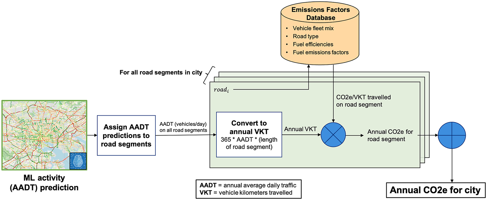
Figure 2. Emissions calculation overview, from ML-predicted AADT to emissions estimate for an entire city.
Total emissions are first computed for each road segment within a city, and then summed to estimate total city emissions (CE) for each GHG:
 $$ \mathrm{CE}=\sum \limits_i{\mathrm{SE}}_i, $$
where
 $ {\mathrm{SE}}_i $
is the “segment emissions” for a road segment
$ {\mathrm{SE}}_i $
is the “segment emissions” for a road segment
 $ i $
. Each
$ i $
. Each
 $ {\mathrm{SE}}_i $
was calculated as:
$ {\mathrm{SE}}_i $
was calculated as:
 $$ {\mathrm{SE}}_i=365\cdot {\mathrm{AADT}}_i\cdot {l}_i\cdot \sum \limits_{v,f}{\eta}_{v,f,{s}_i}\cdot {m}_{v,f,{s}_i}\cdot {g}_{v,f,{s}_i}, $$
where:
 $ {\mathrm{AADT}}_i $
is the average annual daily traffic (unitless vehicles),
$ {\mathrm{AADT}}_i $
is the average annual daily traffic (unitless vehicles),
 $ {l}_i $
is the length of the road segment
$ {l}_i $
is the length of the road segment
 $ i $
in units of km,
$ i $
in units of km,
 $ {\eta}_{v,f,{s}_i} $
is the fuel efficiency, in units of liters per km, for a vehicle type
$ {\eta}_{v,f,{s}_i} $
is the fuel efficiency, in units of liters per km, for a vehicle type
 $ v $
, fuel type
$ v $
, fuel type
 $ f $
and a road segment category
$ f $
and a road segment category
 $ {s}_i $
of the road segment
$ {s}_i $
of the road segment
 $ i $
,
$ i $
,
 $ {m}_{v,f,{s}_i} $
is the vehicle mix, as a fraction, typically present on the road segment based on the vehicle type
$ {m}_{v,f,{s}_i} $
is the vehicle mix, as a fraction, typically present on the road segment based on the vehicle type
 $ v $
, fuel type
$ v $
, fuel type
 $ f $
and a road segment category
$ f $
and a road segment category
 $ {s}_i $
of the road segment
$ {s}_i $
of the road segment
 $ i $
. Specifically, we require that
$ i $
. Specifically, we require that
 $ {\sum}_{v,f}{m}_{v,f,{s}_i}=1 $
for each road segment category
$ {\sum}_{v,f}{m}_{v,f,{s}_i}=1 $
for each road segment category
 $ {s}_i $
. Finally,
$ {s}_i $
. Finally,
 $ {g}_{v,f,{s}_i} $
is the GHG emissions factor, in grams of gas per liter, for the vehicle type
$ {g}_{v,f,{s}_i} $
is the GHG emissions factor, in grams of gas per liter, for the vehicle type
 $ v $
, fuel type
$ v $
, fuel type
 $ f $
and a road segment category
$ f $
and a road segment category
 $ {s}_i $
of the road segment
$ {s}_i $
of the road segment
 $ i $
.
$ i $
.
All three of
 $ {\eta}_{v,f,{s}_i} $
,
$ {\eta}_{v,f,{s}_i} $
,
 $ {m}_{v,f,{s}_i} $
, and
$ {m}_{v,f,{s}_i} $
, and
 $ {g}_{v,f,{s}_i} $
are look-up tables based on data gathered from several sources as described in Section 2.5.
$ {g}_{v,f,{s}_i} $
are look-up tables based on data gathered from several sources as described in Section 2.5.
To calculate a city emissions factor (CEF), we calculated the total city emissions and divided by the total activity, defined as the sum over all road segments of the AADT times length for each segment:
 $$ \mathrm{CEF}=\frac{\mathrm{CE}}{\left(365\cdot \sum \limits_i{\mathrm{AADT}}_i\cdot {l}_i\right)}. $$
As with the CE calculation, we calculate a separate CEF for each of the three major GHGs. Thus, three emissions factor values were provided for each city, representing the average amount of each GHG emitted per kilometer traveled by a single vehicle on any road segment within that city. The units of each provided city emissions factor (CEF) are metric tons (tonnes) of GHG per vehicle kilometer traveled (VKT).
5. Results
We evaluate each ML model on a hold-out test set of U.S. cities, using input data from 2017 to align with the timespan of our ground truth AADT data. We compute the following metrics on a per-road basis: RMSE, MAPE, MPE, and Pearson’s
 $ \rho $
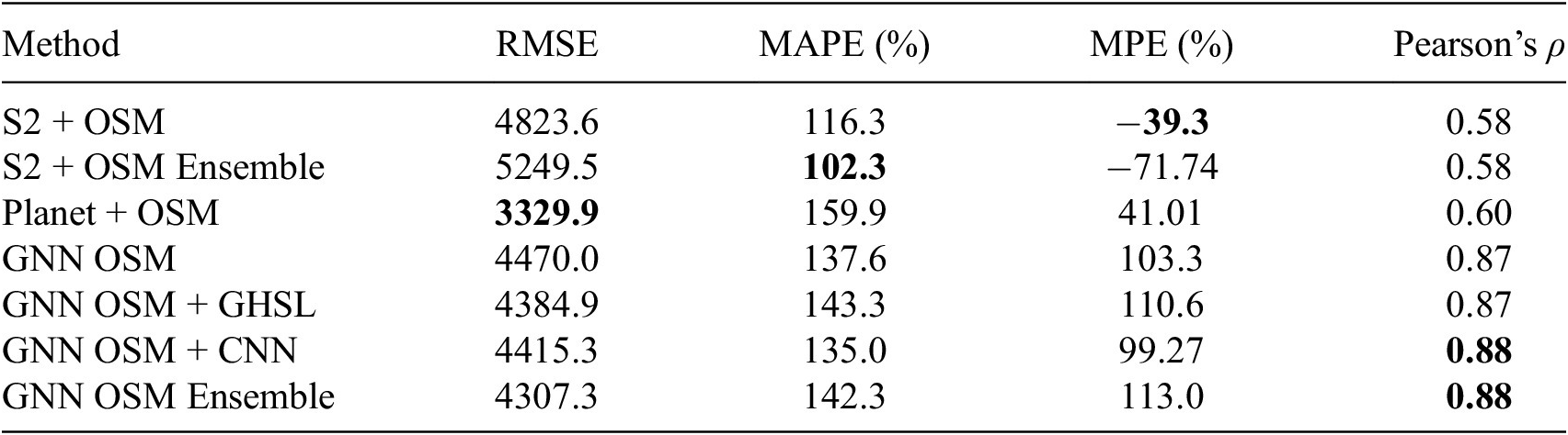
(see Section 3.1 for definitions). Comparing metrics on a per-road basis enables a fair comparison between the image-based CNN models and the graph-based GNN models, as can be seen in Table 5.
$ \rho $
(see Section 3.1 for definitions). Comparing metrics on a per-road basis enables a fair comparison between the image-based CNN models and the graph-based GNN models, as can be seen in Table 5.
Table 5. Comparison of activity prediction models trained with varying inputs and architectures as described in Section 3. Every column has one row bolded to indicate a possible “best” model; see text for a further discussion.
Note. RMSE is in units of vehicles per day.
There is no strong evidence for which model is best, as no one model achieves best performance in more than one metric; each metric in Table 5 has one entry bolded to indicate a possible best model. Furthermore, Table 5 shows evidence to support a trade-off between RMSE and MAPE, and thus likely a trade-off in performance on high-trafficked roads and low-trafficked roads. In general, improvements in the metric more strongly associated with performance on low-trafficked roads (MAPE) results in worse performance on the metric more strongly associated with performance on higher-trafficked roads (RMSE), and vice versa. While MAPE errors are all high, they are not directly indicative of large errors when emissions are calculated at the city level. This is as MAPE is strongly influenced by AADT estimation errors for low-trafficked roads which may be small in an absolute sense, but become large when divided by the ground truth AADT. Also of note is the lower MPE metrics for the CNN models, but the stronger correlation of the GNN models. These all point to the importance of model ensembling to create a more robust activity prediction.
An example of ensemble AADT output can be seen in Figure 3. This map view shows the level of detail afforded by our approach. This output of AADT per road segment is then translated to city-wide emissions as discussed in Section 4.

Figure 3. Example ensembled AADT predictions for the greater Washington, DC area. AADT units are vehicles per day. Map data from OpenStreetMap (Haklay and Weber, Reference Haklay and Weber2008 ).
5.1. International activity prediction
To estimate the ability of our models to generalize outside of the U.S.-based training set, we have run an ensemble of the S2 + OSM CNN and GNN OSM models on 500 global cities, using input data from 2021. Several international AADT datasets are used for evaluation: 26 cities in the United Kingdom (UK) for 2018–2020 (UK 26 Table 7) (Department for Transport, 2020), Buenos Aires, Argentina (Ministry of Transport – National Directorate of Roads, 2017), and Paris, France (Department of Roads, 2021). Per-road AADT error metrics between our ML estimates and these datasets are shown in Table 6, while the list of 26 UK cities is provided in Table 7. Error percentages are generally on par with performance in the U.S., showing the ability of our models to generalize globally.
Table 6. Evaluation of ensembled model output with international AADT

Table 7. List of UK 26 cities used for AADT evaluation

6. Discussion
We have performed several comparisons of our road transportation emissions estimates against other emissions inventories for initial validation, both within the US and globally. A set of 14 hold-out cities in the US was selected for validation with three other emissions inventories: Google Environmental Insights Explorer (EIE) (Google, 2022), Database of Road Transportation Emissions (DARTE) (Gately et al., Reference Gately, Hutyra and Wing2019), and Vulcan v3.0 (Gurney et al., Reference Gurney, Liang, Patarasuk, Song, Huang and Roest2020). Both our CNN and GNN-derived emissions estimates are strongly correlated with other inventory values for every city, with mean Pearson’s
 $ \rho $
values of 0.97 (CNN) and 0.98 (GNN). We also compare our emissions estimates for 500 of the largest global cities to EDGAR (Janssens-Maenhout et al., Reference Janssens-Maenhout, Crippa, Guizzardi, Muntean, Schaaf, Dentener, Bergamaschi, Pagliari, Olivier, Peters, van Aardenne, Monni, Doering, Roxana Petrescu, Solazzo and Oreggioni2017) and Carbon Monitor (Liu et al., Reference Liu, Ciais, Deng, Davis, Zheng, Wang, Cui, Zhu, Dou, Ke, Sun, Guo, Zhong, Boucher, Bréon, Lu, Guo, Xue, Boucher and Chevallier2020). We found strong correlation with both inventories, with Pearson’s
$ \rho $
values of 0.97 (CNN) and 0.98 (GNN). We also compare our emissions estimates for 500 of the largest global cities to EDGAR (Janssens-Maenhout et al., Reference Janssens-Maenhout, Crippa, Guizzardi, Muntean, Schaaf, Dentener, Bergamaschi, Pagliari, Olivier, Peters, van Aardenne, Monni, Doering, Roxana Petrescu, Solazzo and Oreggioni2017) and Carbon Monitor (Liu et al., Reference Liu, Ciais, Deng, Davis, Zheng, Wang, Cui, Zhu, Dou, Ke, Sun, Guo, Zhong, Boucher, Bréon, Lu, Guo, Xue, Boucher and Chevallier2020). We found strong correlation with both inventories, with Pearson’s
 $ \rho $
values of 0.74 and 0.87, respectively, showing the high global accuracy of our method. Further emissions validation details are discussed below.
$ \rho $
values of 0.74 and 0.87, respectively, showing the high global accuracy of our method. Further emissions validation details are discussed below.
6.1. U.S. emissions validation
Google EIE (2022) leverages trip data in combination with emissions factors data to provide emissions estimates for multiple modes of transportation in 42,000+ cities worldwide. We utilize the publicly available 2018 EIE data in the US for our comparison. DARTE (Gately et al., Reference Gately, Hutyra and Wing2019) uses reported vehicular traffic data combined with Census TIGER (Marx, Reference Marx1986) road network information to estimate regional on-road emissions and disaggregate them among mapped road networks. We compare our estimates to both DARTE 2015 and 2017 data. Vulcan (Gurney et al., Reference Gurney, Liang, Patarasuk, Song, Huang and Roest2020) is a national-scale, multi-sectoral, hourly inventory from 2010 to 2015 with a resolution of 1 km2. Vulcan transportation emissions are based on EPA county-level on-road emissions estimates, further downscaled using data from the Federal Highway Administration. We select Vulcan data from 2015 for comparison.
Due to the fact that our ground truth AADT data and satellite imagery for this set of 14 hold-out cities is from 2017, data from the other emissions inventories were selected from years as close to 2017 as possible. We use the geographic bounds available in the EIE data to retrieve satellite imagery and road network data within each city’s bounds. We also constrain our predictions to the same geographic bounds to ensure appropriate comparisons. After predicting AADT with our models and associating AADT with each road segment, road geometries are cropped to the city bounds to create an appropriate estimate of vehicle kilometers traveled (VKT) and emissions for each road. Corresponding emissions estimates from the DARTE and Vulcan raster products are also selected using each city’s EIE bounds.
Several variants of each third-party inventory are examined and shown in Table 8. Google EIE data categorizes trips into three categories: in-boundary, inbound, and outbound. Trips are categorized according to their start and end locations, with in-boundary containing trips that both start and end within city bounds, inbound starting outside and ending inside city bounds, and outbound starting inside and ending outside city bounds. We compare against just in-boundary emissions (EIE_v1_2018), and in-boundary plus 50% inbound and 50% outbound emissions (EIE_v2_2018). For DARTE, we compare against emissions estimates for both 2015 (DARTE_2015) and 2017 (DARTE_2017). Vulcan contains three emissions estimates: the lower 95% confidence interval (Vulcan_lo_2015), mean estimate (Vulcan_mn_2015), and the upper 95% confidence interval (Vulcan_hi_2015).
Table 8. Emissions validation metrics for US cities

Note. MAE and mean error are in units of tonnes CO2, and
 $ \rho $
is Pearson’s
$ \rho $
is Pearson’s
 $ \rho $
.
$ \rho $
.
For each of the 14 hold-out cities we use for validation, we plot the distribution of values from Vulcan, DARTE, and EIE along with the mean in Figure 4. Here the box plot shows the mean, and the 25–75% distribution. Estimates based on our CNN and GNN models are shown as dots and x’s.

Figure 4. Distribution of emissions estimates for each US city using values from DARTE, Vulcan, and Google’s EIE as described in Table 8. Emissions estimates based on our S2 + OSM CNN are marked with red dots, and estimates based on our GNN OSM model outputs are marked with blue X’s.
6.2. Global emissions validation
Initial validation was performed for our global emissions estimates, where we compared against both EDGAR (Janssens-Maenhout et al., Reference Janssens-Maenhout, Crippa, Guizzardi, Muntean, Schaaf, Dentener, Bergamaschi, Pagliari, Olivier, Peters, van Aardenne, Monni, Doering, Roxana Petrescu, Solazzo and Oreggioni2017) and Carbon Monitor city-level data for 2018–2020 (Liu et al., Reference Liu, Ciais, Deng, Davis, Zheng, Wang, Cui, Zhu, Dou, Ke, Sun, Guo, Zhong, Boucher, Bréon, Lu, Guo, Xue, Boucher and Chevallier2020). EDGAR 2015 data is retrieved from the Global Human Settlement Layer-Urban Centres Database (GHSL-UCDB) dataset (Florczyk et al., Reference Florczyk, Corbane, Schiavina, Pesaresi, Maffenini, Melchiorri, Politis, Sabo, Freire, Ehrlich, Kemper, Tommasi, Airaghi and Zanchetta2019) from which we have selected our set of 500 global cities, and we acknowledge that more recent EDGAR data from 2018 should be used in future validation experiments. Carbon Monitor is a recent emissions inventory that utilizes a variety of activity data sources to estimate emissions in multiple sectors on a daily basis. In addition to country-level data, Carbon Monitor has released near real-time emissions estimates for 52 cities globally. This city-level data is used in our analysis, for 50 total cities that overlap the global set of 500 cities for which we have produced emissions estimates.
Validation metrics for both dataset comparisons are shown in Table 9. The resulting comparison for all 500 cities against EDGAR can be seen in Figure 5. While the Pearson’s
 $ \rho $
value of 0.74 indicates decent correlation, the wide variance of the differences is noteworthy and warrants further investigation. The sharp “wall” on the left portion of the plot is caused by the fact that our 500 cities were selected based on thresholded EDGAR 2015 estimates.
$ \rho $
value of 0.74 indicates decent correlation, the wide variance of the differences is noteworthy and warrants further investigation. The sharp “wall” on the left portion of the plot is caused by the fact that our 500 cities were selected based on thresholded EDGAR 2015 estimates.
Table 9. Global emissions validation metrics for our estimates compared with EDGAR (Janssens-Maenhout et al., Reference Janssens-Maenhout, Crippa, Guizzardi, Muntean, Schaaf, Dentener, Bergamaschi, Pagliari, Olivier, Peters, van Aardenne, Monni, Doering, Roxana Petrescu, Solazzo and Oreggioni2017) and Carbon Monitor (Liu et al., Reference Liu, Ciais, Deng, Davis, Zheng, Wang, Cui, Zhu, Dou, Ke, Sun, Guo, Zhong, Boucher, Bréon, Lu, Guo, Xue, Boucher and Chevallier2020) data

Note. MAE and mean error are in units of tonnes CO2.

Figure 5. Our emissions estimates for 500 global cities compared with EDGAR 2015 data. Note that axes are in log scale.
The results of the comparison with the 50 overlapping Carbon Monitor cities for 2021 are shown in Figure 6. There is generally good alignment between the two sets of emissions, with some larger differences in France (Nice, Lyon, Marseille), South America (Bogota, São Paulo), Russia (Saint Petersburg, Moscow), and India (Mumbai, Delhi). We also note the larger percentage errors for 2020 in Table 9 as compared to 2019 and 2021, likely due to COVID-19 lockdown effects.

Figure 6. Our emissions estimates for 50 global cities compared with Carbon Monitor 2021 data. Note that axes are in log scale.
7. Conclusion
We have presented a hybrid road transportation emissions estimation method that is accurate, scalable, and easy to update. The ability to calculate emissions per road segment can be further refined to reach an unprecedented level of detail and global coverage. Where available, the integration of real-time traffic data would increase the temporal resolution and accuracy of our models. We also plan to carry out further analysis of our emissions estimates with other inventories to identify the main causes of discrepancies. As well, we aim to explore open-sourcing our emissions factors schema such that governments and other entities can contribute more up-to-date and accurate EF data to further improve our estimates. This type of actionable emissions monitoring data will be critical to ensuring we meet global emissions reduction targets and may inspire new ways of mitigating the effects of climate change.
Acknowledgments
We would like to thank the Climate TRACE coalition, WattTime, Google.org, Generation Investment Management, and Al Gore for their organizational and financial support. Additional thanks to Dr. Kevin Gurney, Northern Arizona University, for his continuous feedback and review of our methodology.
Author contribution
Conceptualization: D.R., M.H.; Data curation: K.F., T.M.K.; Methodology: D.R., M.H., K.F.; Software: Ro.M., Ra. M., N.F., C.A., F.W., D.R.; Writing: D.R., T.M.K., K.F., N.F., E.P.R.
Competing interest
The authors declare none.
Data availability statement
Global estimates of greenhouse gas emissions from road transportation in the top 500 cities are available at https://climatetrace.org/.
Ethics statement
The research meets all ethical guidelines, including adherence to the legal requirements of the study country.
Funding statement
The authors would like to thank WattTime and the Climate TRACE coalition for their organizational support, and Climate TRACE funders—Al Gore, Generation Investment Management, Google.org, and Patrick J. McGovern Foundation.


 Open access