


1. Introduction
Internal flow represents an important class of fluid dynamics problems involving flow through an object or device with one or more inflows and exit flows. Many exact or approximate analytical solutions are known for certain simplified conditions that provide the basis for understanding internal flow physics. These solutions are also important in design for many applications, including flow-network modelling (Sultanian Reference Sultanian2018), gas-turbine engines (Farokhi Reference Farokhi2014; Sultanian Reference Sultanian2018), gas pipelines (John & Keith Reference John and Keith2006), rockets (Sutton & Biblarz Reference Sutton and Biblarz2010) and industrial air systems (Taheri & Gadow Reference Taheri and Gadow2017). The present paper describes a new, closed-form solution for steady, compressible internal flow problems that includes arbitrary forces (including friction), heat transfer, area change, flow non-uniformity and multiple inlet/exit flows.
The simplest internal flows can be considered as steady, with a single inlet and a single exit. Flow non-uniformity is generally ignored, hence these are often referred to as ‘one-dimensional’ or ‘quasi-one-dimensional’ solutions. These solutions are derived from either the differential form or the integral form of the governing equations. Examples of solutions derived from the differential form include Fanno flow (constant area flow with friction), Rayleigh flow (constant area flow with heat transfer) and isentropic flow with area change. The normal shock relations are an example of a solution derived from the integral form. In each of these examples, the analysis provides a one-dimensional solution where the effect of a single physical parameter is modelled.
Many texts provide analysis of one-dimensional, internal flow problems that involve some combination of friction, heat transfer and area change. Numerical methods are often provided, but closed-form solutions are less common. Shapiro (Reference Shapiro1953) studied general compressible flow with friction, heat addition and area change using the differential form of the governing equations. However, no exact, closed-form solution was identified, although some approximations and simplifications were discussed in detail.
Recently, Ferrari (Reference Ferrari2021a,Reference Ferrarib) presented two closed-form solutions to the one-dimensional differential equations. The first is the case of constant area with combined heat transfer and friction, and the second is for conical area change with friction. The former was shown to agree with the classical Rayleigh and Fanno solutions. Numerical simulations for combined friction and heat transfer were shown to agree with the closed-form solution. Additionally, the assumption of constant heat transfer could be replaced with a wall temperature boundary condition, but the solution procedure would become iterative rather than closed-form. The solution for area change with friction was shown to agree with numerical solutions.
The control volume approach, using the integral form of the governing equations, is more common in the literature for solving quasi-one-dimensional, compressible flow problems. Crocco (Reference Crocco and Emmons1958) studied compressible flow with friction, heat addition and area change using the integral form of the governing equations. A pressure–area power-law relationship was assumed, where the static pressure ratio was assumed to be a function of the area ratio with some constant exponent. This allowed the wall pressure force to then be evaluated in the integral form of the momentum balance. This particular approach has seen use in scramjet combustors (Curran, Heiser & Pratt Reference Curran, Heiser and Pratt1996). Dobrowolski (Reference Dobrowolski1966) used Crocco's pressure–area relationship to solve the problem of one-dimensional, compressible flow with simultaneous area change and heat transfer. Loh (Reference Loh1970) expanded this approach to include the effect of friction. Later, Greitzer, Tan & Graf (Reference Greitzer, Tan and Graf2004) also discussed many solutions to various one-dimensional flows, including incompressible sudden expansions, incompressible sudden contractions, and mixing of two compressible flows. John & Keith (Reference John and Keith2006) discussed simultaneous friction, heat transfer and area change, but solved the problem using a numerical approximation. Similarly, Farokhi (Reference Farokhi2014) used the integral form of the governing equations and found a quadratic solution in exit Mach number squared to the problem of heat transfer and drag in a constant area duct. Kundu, Cohen & Dowling (Reference Kundu, Cohen and Dowling2015) also used the integral form of the governing equations and found a quadratic solution in exit Mach number squared to the problem of heat transfer and friction in a constant area duct; however, the friction force was not coupled to the dynamic pressure.
Denton (Reference Denton1993) applied the integral form of the governing equations to flows involving turbomachinery. An iterative solution procedure was derived for the mixing of two streams, but a closed-form solution was not obtained. Denton (Reference Denton1993) also studied the diffusion of aerofoil wakes in axial turbines and compressors. Trends and qualitative behaviour were identified based on boundary-layer quantities at the aerofoil trailing edge. Rose & Harvey (Reference Rose and Harvey1999) studied a similar problem involving the mixing of a wake in a turbine that had a non-uniform total temperature. They used the control volume approach and the integral form of the governing equations in order to obtain a quadratic solution in exit velocity.
An internal flow in which two supersonic streams mix together has been studied by Fabri & Paulon (Reference Fabri and Paulon1958), Chow & Addy (Reference Chow and Addy1964) and Dutton, Mikkelsen & Addy (Reference Dutton, Mikkelsen and Addy1982). Each work used experimental results compared to theoretical predictions in order to draw conclusions about the flow physics. Fabri & Paulon (Reference Fabri and Paulon1958) saw reasonable agreement between predictions and experimental results using a steady one-dimensional approach using the integral form of the governing equations. Chow & Addy (Reference Chow and Addy1964) noted some limitations with the Fabri & Paulon (Reference Fabri and Paulon1958) approach. They improved the prediction by including detailed computer calculations of the inviscid interactions of the two-streams and viscous effects using the differential form of the governing equations. Dutton et al. (Reference Dutton, Mikkelsen and Addy1982) showed a closed-form solution in exit Mach number squared based on a similar approach by Fabri & Paulon (Reference Fabri and Paulon1958). However, the prediction neglected viscous effects, including wall friction, and was shown to have significant differences compared to data.
The problem of compressible internal flow undergoing a sudden expansion (also called sudden enlargement) was shown to have an exact, closed-form solution by Hall & Orme (Reference Hall and Orme1955). This approach used the integral form of the governing equations and found an exact solution in the form of a quadratic in exit Mach number squared. This prediction was then compared to experimental data, and the agreement was found to be excellent. The choice of positive or negative root in the sudden expansion quadratic solution was explored in additional detail by Woods & Daneshyar (Reference Woods and Daneshyar1965). The similar problem of compressible internal flow undergoing sudden contraction was investigated by Benedict, Carlucci & Swetz (Reference Benedict, Carlucci and Swetz1966) and Marjanovic & Djordjevic (Reference Marjanovic and Djordjevic1994). Theoretical predictions were found to deviate appreciably from experimental data. Empirical relations were found to be required in order to improve the accuracy of predictions.
Heiser et al. (Reference Heiser, Pratt, Mehta and Daley1994) studied hypersonic external flows using a control volume with area change, heat addition and a wall force, where one of the control surfaces was a streamline. This approach also used the integral form of the governing equations. It was found that the solution was a quadratic in exit velocity. The wall force included both viscous and wall pressure effects. However, the intent of that solution was for external flows. Hence guidance was not provided on how to approximate the wall forces. Additionally, the solution did not include the ability to accommodate non-uniform profiles at the boundaries.
The intent of the present work was to combine the effects of arbitrary area change, heat transfer, friction and flow non-uniformity into a single, closed-form analytical solution. It is the inclusion of all of these effects that makes this approach unique and distinct from the cited literature. The subsequent sections of this paper will develop a control volume formulation with a closed-form solution. Example problems will then be used to first show consistency with known solutions. This is followed by a description of several unique internal flow solutions that will be compared with data available in the literature.
2. Set-up
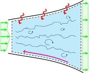
The approach uses a control volume with a combination of heat transfer, friction and area change. A control volume that illustrates this combination is shown in figure 1. The surface of the control volume is divided into the inlet, the outlet and an impermeable wall. Additionally, there is no mass flow or velocity component normal to the wall. The flow properties are not assumed uniform across any control surface.

Figure 1. Control volume with simultaneous heat transfer, friction and area change.
The problem considers the  $x$-direction momentum equation only. Further, the problem is assumed to be steady with only the
  $x$-component of velocity being non-zero at the inlet and exit locations. Additionally, the calorically perfect ideal gas assumption is used, which implies that the specific heats
  $c_P$ and
  $c_{\mathcal {V}}$ are constant, and the ideal gas law
  $P = \rho R T$ applies. The Mach number is given as
  $M = \sqrt {\gamma R T}$. The ratio of the stagnation enthalpy (
 $h_{o} \equiv h + {V^2}/{2}$) to the static value for a calorically perfect gas is
 \begin{equation} \frac{h_o}{h} = \frac{T_o}{T} = 1 + \frac{\gamma -1}{2}\,M^2 \equiv f(M),\end{equation}
where the function  $f(M)$ is defined for convenience as it appears frequently in the analysis.
An important aspect of the analytical solution presented below is the ability to consider components in which the inflow or exit flow has non-uniform conditions. This non-uniformity could apply to any flow field variable, including velocity, density and temperature. Fluid variables at the inlet and exit of the control volume will be represented by appropriate average values. This will include conditions where more than one inflow stream is present, by considering a single inflow boundary with non-uniform conditions.
Two types of averaging will be considered here: the area average and the mass average. The area average of a quantity  $\varphi$ is defined as
 \begin{equation} \bar{\varphi}^A \equiv \frac{1}{A} \int \varphi\, {\rm d} A. \end{equation}
The mass average of a quantity  $\varphi$ is defined as
 \begin{equation} \bar{\varphi}^m \equiv \frac{1}{\dot{m}} \int \rho \varphi ( \boldsymbol{V} \boldsymbol{\cdot} \hat{\boldsymbol{n}})\, {\rm d} A. \end{equation}
Note that many other types of averages could be considered, as discussed in Cumpsty & Horlock (Reference Cumpsty and Horlock2005), and the choice of a particular averaging type is based on how it helps to simplify the analysis. Pressure, for example, most often appears in this analysis as an area average,  $\bar {P}^A$, as this replaces an integral quantity that occurs naturally in the momentum equation (Cumpsty & Horlock Reference Cumpsty and Horlock2005). Similarly, the mass-averaged value of stagnation enthalpy,
  $\bar {h}^{m}_o$, replaces an integral that occurs in the control volume energy equation (Cumpsty & Horlock Reference Cumpsty and Horlock2005). The mass-averaged stagnation temperature for a calorically perfect ideal gas may then be calculated as
 \begin{equation} \bar{T}^m_o = \frac{\bar{h}^m_o}{c_P}. \end{equation}
 For the present work, a combination of area averaging and mass averaging will be used most often. In cases where neither area or mass averaging is specified, a simple overbar will be used:  $\overline {({\cdot })}$. Note that for uniform flows, the use of averaging is not required since all relevant quantities are constant along that particular control surface, and the overbar notation can be neglected, i.e.
  $\bar {\varphi }^A = \bar {\varphi }^m = \varphi$. Mass, area or any other averaging can be used for the Mach number, so it is left as
  $\bar {M}$. The solution will remain exact with this arbitrarily chosen average
  $\bar {M}$ by using ‘flux correction factors’, which are discussed later. Thus one should choose an averaging technique for
  $\bar {M}$ that provides convenience for the problem of interest.
The use of area-averaged static pressure, mass-averaged stagnation temperature, an average Mach number, and flux correction factors allows the problem to be solved for both uniform and non-uniform quasi-one-dimensional flow problems. The following quantities are defined so that integral forms of mass, momentum and energy conservation are visually similar to their uniform flow counterparts. The function  $\tilde {f}$ is analogous to the stagnation-to-static enthalpy ratio and is defined as
 \begin{equation} \tilde{f} \equiv 1 + \frac{\gamma - 1}{2}\,\bar{M}^2. \end{equation}
Note that  $\tilde {f}$ is not an average quantity itself; rather, it is defined using other average quantities. A representative static temperature can then be defined as
 \begin{equation} \tilde{T} \equiv \frac{\bar{T}^m_o}{\tilde{f}}. \end{equation}
A representative static density can then be defined as
 \begin{equation} \tilde{\rho} \equiv \frac{\bar{P}^A}{R\tilde{T}} = \frac{\bar{P}^A}{R}\, \frac{\tilde{f}}{\bar{T}^m_o}. \end{equation}
A representative velocity can then be defined as
 \begin{equation} \tilde{V} \equiv \bar{M} \sqrt{\gamma R \tilde{T}} = \bar{M} \sqrt{\gamma R\,\frac{\bar{T}^m_o}{\tilde{f}}}. \end{equation}
Similar to  $\tilde {f}$, the quantities
  $\tilde {T}$,
  $\tilde {\rho }$ and
  $\tilde {V}$ are not average quantities themselves; rather, they are representative quantities defined in terms of other averages, i.e.
  $\bar {P}^{A}$,
  $\bar {T}^m_o$ and
  $\bar {M}$. They are analogous to their uniform-flow counterparts
  $f$,
$f$,  $T$,
$T$,  $\rho$ and
  $V$. The use of these definitions allows the formulation to be mathematically exact while maintaining a familiar form to the equations.
Conventionally, integral quantities in the control volume formulations with non-uniform profiles are represented using flux correction factors (also called non-uniformity coefficients). These are scalars that serve to modify values computed from spatially averaged quantities in order to preserve an integrated quantity of interest, e.g. momentum flux. Correction factors for compressible flow are discussed in Crocco (Reference Crocco and Emmons1958). For incompressible flow, these factors are described in more detail in White (Reference White2006) and Munson et al. (Reference Munson, Huebsch, Rothmayer, Gerhart, Gerhart and Hochstein2015).
The mass flux correction factor is defined here as
 \begin{equation} \alpha \equiv \frac{\displaystyle \int \rho ( \boldsymbol{V} \boldsymbol{\cdot} \hat{\boldsymbol{n}})\, {\rm d} A}{\tilde{\rho}\tilde{V}A}. \end{equation}
This term is equal to unity for constant density flows when using an area-averaged velocity. However, when the density is not spatially uniform, it is possible for  $\alpha$ to be greater than or less than unity. For example, if spatial variations in
  $\rho$ and
  $V$ are positively correlated over the inlet surface, then the mass flow rate is
  $\dot {m} > \tilde {\rho }\tilde {V}A$, hence
  $\alpha > 1$. Similarly, if density and velocity variations are negatively correlated over the area, then
  $\alpha < 1$. Inserting the definitions of
  $\tilde {\rho }$ and
  $\tilde {V}$ shows its dependence on normalized profiles of static pressure, stagnation temperature, Mach number and stagnation-to-static enthalpy:
 \begin{equation} \alpha = \frac{1}{A} \int \frac{P}{\bar{P}^A} \left(\frac{T_o}{\bar{T}^m_o} \right)^{-{1}/{2}} \frac{\ M\ }{\bar{M}} \sqrt{\frac{\ f\ }{\tilde{f}}}\, {\rm d} A.\end{equation}
This provides a useful method to estimate  $\alpha$ values if there is knowledge regarding the shapes of the relevant dimensionless profiles.
The momentum flux correction factor is defined as
 \begin{equation} \beta \equiv \frac{\displaystyle \int \rho V ( \boldsymbol{V} \boldsymbol{\cdot} \hat{\boldsymbol{n}} )\, {\rm d} A}{\tilde{\rho}\tilde{V}^2 A}. \end{equation}
This follows from the classical definition given in White (Reference White2006) and Munson et al. (Reference Munson, Huebsch, Rothmayer, Gerhart, Gerhart and Hochstein2015). Substituting the definitions of  $\tilde {\rho }$ and
  $\tilde {V}$ shows its dependence on the normalized profiles of static pressure and Mach number:
 \begin{equation} \beta = \frac{1}{A} \int \frac{P}{\bar{P}^A} \left(\frac{\ M }{\bar{M}}\right)^2 {\rm d} A. \end{equation}
Thus the momentum flux correction factor can be evaluated as the area average of a combination of the normalized profiles over the control surface.
These flux correction factors allow for any averaging method to be used for  $\bar {M}$. It requires only consistent use throughout the equations. Careful selection of the averaging method can guarantee certain properties of
  $\beta$. For example, using Schwarz's inequality, it can be shown that if
  $\bar {M} = \bar {M}^A$, then
  $\beta \geq 1$.
3. Derivation of control volume solution
The conservation of mass for a steady, single-inlet, single-exit control volume is given as
 \begin{equation} \alpha_ 2 \tilde{\rho}_2 \tilde{V}_2 A_2 - \alpha_1 \tilde{\rho}_1 \tilde{V}_1 A_1 = 0, \end{equation}
where the subscript 2 represents exit conditions, and the subscript 1 indicates inlet conditions.
Substituting the ideal gas law and the definition of the Mach number into (3.1), and using (2.1), gives
 \begin{equation} \frac{\bar{P}_2^A A_2}{\bar{P}_1^A A_1}\,\frac{\alpha_2}{\alpha_1} \sqrt{\frac{\bar{T}_{o1}^m}{\bar{T}_{o2}^m}}\,\frac{\bar{M}_2}{\bar{M}_1} \left( \frac{\tilde{f}_2}{\tilde{f}_1} \right)^{1/2} - 1 = 0.\end{equation}
It should be noted that in (3.2), the static pressure is used rather than the stagnation pressure. Further, the stagnation temperature is used rather than the static temperature. The reason for this choice is that the static pressure and stagnation temperature occur in the momentum and energy equations, respectively. Additionally, the pressure occurs with an integer exponent. Thus those equations require no additional manipulation for all three governing equations to contain the same set of unknown quantities.
The steady  $x$-momentum balance equation is
 \begin{equation} \beta_2 \tilde{\rho}_2 \tilde{V}_2^2 A_2 - \beta_1 \tilde{\rho}_1 \tilde{V}_1^2 A_1 = \bar{P}_1^A A_1 - \bar{P}_2^A A_2 + \bar{P}_3^A ( A_2 - A_1 ) - F_{fx}, \end{equation}
where  $\bar {P}_1^A$ and
  $\bar {P}_2^A$ represent the area-averaged static pressure on inlet and outlet control surfaces, respectively. Here,
  $F_{fx}$ is the friction force acting on the control volume projected in the
  $x$-direction. The term
  $\bar {P}_3^A (A_2-A_1)$ represents the axial force on the fluid due to the wall pressure. Therefore,
  $\bar {P}_3^A$ represents an average over the projected area of the walls of the device.
The area-averaged wall pressure  $\bar {P}_3^A$ will be of primary importance in the solution for any problems that involve area change. In many cases, this term will be the only unknown needed for closure of the equations, hence it must be specified in order to solve for the control volume exit conditions. Without loss of generality,
  $\bar {P}_3^A$ may be prescribed as a linear combination of the inlet static pressure
  $\bar {P}_1^A$, the exit static pressure
  $\bar {P}_2^A$, and an average inlet stagnation pressure
  $\bar {P}_{o1}$:
 \begin{equation} \frac{\bar{P}_3^A}{\bar{P}_1^A} = (1-\xi-\nu) + \xi\, \frac{\bar{P}_2^A}{\bar{P}_1^A} + \nu\, \frac{\bar{P}_{o1}}{\bar{P}_1^A},\end{equation}
where  $\xi$ and
  $\nu$ represent wall-pressure scaling coefficients. Note that the wall pressure was prescribed in terms of the known inlet conditions and the unknown outlet static pressure, similar to Shapiro (Reference Shapiro1953) and John & Keith (Reference John and Keith2006). Therefore, the wall pressure is prescribed implicitly. This leads to a closed-form solution for the exit conditions rather than an iterative solution. Determining the appropriate wall-pressure scaling coefficients for various problems is discussed in later sections.
The net friction force per unit area is written as a friction coefficient multiplied by  $\frac {1}{2} \rho V^2$. The net friction force is then calculated by integrating over the wall area and taking the
  $x$-component of the resulting force. The integration of
  $\frac {1}{2} \rho V^2$ cannot be performed directly, thus the integral is approximated using the mean of the inlet and outlet
  $\rho V^2$ values:
 \begin{equation} F_{fx} \equiv \int_1^2 \frac{c_f}{2}\,\rho V^2 \cos(\theta_3)\, {\rm d} A_3 \approx \frac{c_f}{4}\,\gamma ( \beta_1 \bar{P}_1^A \bar{M}_1^2 + \beta_2 \bar{P}_2^A \bar{M}_2^2 ) A_{3f}, \end{equation}
where  $c_f$ is the friction coefficient,
  $\theta _3$ is the angle from the
  $x$-direction to the wall, and
  $A_{3f}$ is defined as
 \begin{equation} A_{3f} \equiv \int_1^2 \cos(\theta_3)\, {\rm d} A_3. \end{equation}
The momentum equation then becomes
 \begin{align} &1 + \beta_1 \gamma \left(1 - \frac{c_f}{4}\,\frac{A_{3f}}{A_1} \right) \bar{M}_1^2 + \left(1-\xi + \nu \left( \frac{\bar{P}_{o1}}{\bar{P}_1^A} - 1 \right) \right) \left( \frac{A_2}{A_1} - 1\right) \nonumber\\ &\quad =\frac{\bar{P}_2^A A_2}{\bar{P}_1^A A_1} \left( 1 + \beta_2 \gamma \left(1 + \frac{c_f}{4}\,\frac{A_{3f}}{A_2} \right) \bar{M}_2^2 + \xi \left( \frac{A_1}{A_2} - 1 \right)\right). \end{align}
The steady energy conservation equation without power transfer across the control surface, consistent with figure 1, is
 \begin{equation} \bar{h}_{o2}^m - \bar{h}_{o1}^m = \frac{\dot{Q}}{\dot{m}} \equiv q.\end{equation}
This can be written in terms of stagnation temperature as
 \begin{equation} \frac{\bar{T}_{o2}^m}{\bar{T}_{o1}^m} = \frac{q}{\bar{h}_{o1}^m} + 1.\end{equation}
 Substitution of (3.9) into (3.2), solving for  $(\bar {P}_2^A A_2 ) / (\bar {P}_1^A A_1)$, and substitution into (3.7) results in
 \begin{align} &\frac{ 1 + \beta_1 \gamma \left(1 - \dfrac{c_f}{4}\, \dfrac{A_{3f}}{A_1} \right) \bar{M}_1^2 + \left(1-\xi + \nu \left( \dfrac{\bar{P}_{o1}}{\bar{P}_1^A} - 1 \right) \right) \left( \dfrac{A_2}{A_1} - 1\right)}{\dfrac{\alpha_1}{\alpha_2}\,\bar{M}_1 \sqrt{\tilde{f}_{1} \left( \dfrac{q}{\bar{h}_{o1}^m} + 1 \right)}}\nonumber\\ &\quad =\frac{1 + \beta_2 \gamma \left(1 + \dfrac{c_f}{4}\, \dfrac{A_{3f}}{A_2} \right) \bar{M}_2^2 + \xi \left( \dfrac{A_1}{A_2} - 1 \right)}{\bar{M}_2 \sqrt{\tilde{f}_{2}}}. \end{align}
All conditions at the inlet are assumed to be known, as well as the friction coefficient, heat transfer and wall-pressure scaling coefficients for cases with area change. Equation (3.10) thus contains only a single unknown:  $\bar {M}_2$. Squaring both sides of (3.10) and simplifying results in the quadratic equation
 \begin{equation} (\bar{M}_2^2)^2 + b (\bar{M}_2^2) + c =0.\end{equation}
The quadratic coefficients are
 \begin{equation}
\left.\begin{array}{c} b \equiv
\dfrac{\varLambda - 2\gamma \beta_2 \left[ 1 + \xi
\left(\dfrac{A_1}{A_2} - 1\right)\right] \left( 1 +
\dfrac{c_f}{4}\, \dfrac{A_{3f}}{A_2}
\right)}{\varLambda\,\dfrac{\gamma - 1}{2} - \left[\gamma
\beta_2 \left( 1 + \dfrac{c_f}{4}\,\dfrac{A_{3f}}{A_2}
\right) \right]^2} \\
\text{and} \quad c
\equiv{-}
\dfrac{\left[ 1 + \xi \left(\dfrac{A_1}{A_2} -
1\right)\right]^2}{\varLambda\,\dfrac{\gamma - 1}{2} -
\left[\gamma \beta_2 \left( 1 +
\dfrac{c_f}{4}\,\dfrac{A_{3f}}{A_2} \right) \right]^2},
\end{array}\right\}
\end{equation}
\begin{equation}
\left.\begin{array}{c} b \equiv
\dfrac{\varLambda - 2\gamma \beta_2 \left[ 1 + \xi
\left(\dfrac{A_1}{A_2} - 1\right)\right] \left( 1 +
\dfrac{c_f}{4}\, \dfrac{A_{3f}}{A_2}
\right)}{\varLambda\,\dfrac{\gamma - 1}{2} - \left[\gamma
\beta_2 \left( 1 + \dfrac{c_f}{4}\,\dfrac{A_{3f}}{A_2}
\right) \right]^2} \\
\text{and} \quad c
\equiv{-}
\dfrac{\left[ 1 + \xi \left(\dfrac{A_1}{A_2} -
1\right)\right]^2}{\varLambda\,\dfrac{\gamma - 1}{2} -
\left[\gamma \beta_2 \left( 1 +
\dfrac{c_f}{4}\,\dfrac{A_{3f}}{A_2} \right) \right]^2},
\end{array}\right\}
\end{equation}
where the term  $\varLambda$ was introduced only for brevity as
 \begin{equation} \varLambda \equiv \left[\dfrac{ 1 + \beta_1 \gamma\left(1 - \dfrac{c_f}{4}\, \dfrac{A_{3f}}{A_1} \right) \bar{M}_1^2 + \left(1-\xi + \nu \left( \dfrac{\bar{P}_{o1}}{\bar{P}_1^A} - 1 \right)\right)\left( \dfrac{A_2}{A_1} - 1\right) }{\dfrac{\alpha_1}{\alpha_2}\,\bar{M}_1 \sqrt{\tilde{f}_{1} \left( \dfrac{q}{\bar{h}_{o1}^m} + 1 \right)}}\right]^2.\end{equation}
Physically,  $\varLambda$ is the squared sum of all known momenta non-dimensionalized by the square of the mass flow rate and the stagnation enthalpy. This can be shown to be equivalent to the non-dimensionalization presented by Denton (Reference Denton1993) and Greitzer et al. (Reference Greitzer, Tan and Graf2004) for the two-stream mixing problem.
4. Solution procedure
The unknown exit Mach number represents the full solution. This can now be found from the quadratic equation as
 \begin{equation} \bar{M}_2^2 ={-}\frac{b}{2} \pm \sqrt{\left(\frac{b}{2}\right)^2 - c}.\end{equation}
This represents a closed-form algebraic solution to the generalized internal flow problem that does not require a numerical solution or iterative methods.
The final issue to consider is that the solution was obtained from a bi-quadratic, and hence allows for four roots as potential solutions. Physically realizable solutions may be determined by considering two restrictions. First, the exit Mach number must be a real positive number. This requirement eliminates all roots for which  $\bar {M}_2 < 0$ (i.e. reversed outlet flow),
  $\bar {M}_2^2 <0$ and
  $(b/2)^2 - c < 0$ (i.e. imaginary
  $\bar {M}_2$). A single solution is possible for any real
  $b$ value given that
  $|b/2| < \sqrt { ( b/2)^2 - c}$ . Two solutions are possible if
  $b<0$ and
  $|b/2| > \sqrt { ( b/2)^2 - c}$. Whether or not these possible solutions will be supersonic or subsonic will depend on
  $|{-b/2} - 1|$,
  $\sqrt {( b/2)^2-c}$, and the choice of ‘
 $\pm$’. Hereafter, the choice ‘
 $+$’ will be referred to as a ‘positive root’, and ‘
 $-$’ will be referred to as a ‘negative root’. The results are summarized in table 1. The final restriction requires eliminating non-physical solutions by satisfying the second law:
 \begin{equation} {\rm \Delta} s \ge \int_1^2 \frac{\delta q}{T}.\end{equation}
Table 1. Conditions for  $\bar {M}_2$ solutions.

The stated restrictions reduce the number of allowable solutions to either one or two. In the event that two  $\bar {M}_2$ solutions are obtained, both should be considered to be physically realizable for the boundary conditions provided, e.g. one subsonic and one supersonic. This will be demonstrated in the following sections, with examples of both canonical flow problems and several unique solutions that were made possible by the formulation given by (3.11).
Once the solution for  $\bar {M}_2$ is known, all other quantities at the exit may be obtained. For example, the exit pressure
  $\bar {P}_2^A$ can be found from the conservation of mass, i.e. (3.1). Hence all exit conditions, including entropy change, can be found from the solution.
The control volume solution as derived can be used for any internal flow component, as long as the required inputs are known or can be approximated. However, there may be cases where there is an advantage to dividing the flow into multiple sub-elements in the streamwise direction. An example of this is very long geometries with friction, such as long pipe flow problems. In this case, the approximation to the friction force given by (3.5) is improved if the component is segmented into multiple short sections. The control volume solution still provides a closed-form solution, but a streamwise-direction marching approach is applied. This provides a closed-form solution to the discretized problem, which is defined as ‘semi-analytical’ (De Vidts & White Reference De Vidts and White1992). This can be shown to provide second-order convergence with increasing sub-element count.
A second example where multiple sub-elements may be useful is for flows with continuously varying cross-sectional area in which the wall-pressure scaling ( $\xi$) is unknown. The wall-pressure scaling is set to
  $\xi =1/2$,
  $\nu =0$, which approximates the wall pressure as the mean of inlet and outlet static pressure. This is commonly used with the steady one-dimensional differential equations (Shapiro Reference Shapiro1953; John & Keith Reference John and Keith2006; Kundu et al. Reference Kundu, Cohen and Dowling2015). Effectively, this means that the wall pressure is being solved for along the length of overall control volume. Like the case of friction, this can be shown to provide second-order convergence with increasing sub-element count. Convergence to the solution occurs regardless of the value of
  $\xi$ as long as
  $\nu =0$, though the rate of convergence varies with the actual value of
  $\xi$. This result indicates that in the limit of infinitely many sub-elements (i.e. a differential size control volume), the solution presented in this work is consistent with the solution of the differential form of the governing equations for steady, compressible, quasi-one-dimensional flow.
Problems that include arbitrary area change may be solved with a single control volume provided that the values of  $\xi$ and
  $\nu$ are given. For example, in a flow with gradual area change, it may be assumed that the wall pressure varies between the inlet and exit static pressure values. This would be independent of the inlet stagnation pressure. Hence
  $\nu =0$, and choosing
  $\xi$ in the range
  $0 \leq \xi \leq 1$ will set
  $\bar {P}_3^A$ between the inlet and exit static pressures. In problems where the inlet stagnation pressure is more appropriate, with a relevant constraint
  $1 - \xi - \nu = 0$, and choosing
  $0 \leq \nu \leq 1$, will set
  $\bar {P}_3^A$ between the exit static pressure and the inlet stagnation pressure. Two examples, which set
  $\xi$ and
  $\nu$ within these ranges, are the cases of sudden expansion and sudden contraction. These are discussed in § 6.
Alternatively, if the values of  $\xi$ and
  $\nu$ are not readily apparent from the geometry, the values may be varied over some range and selected to achieve a specific outlet condition. For example, a known component efficiency or entropy generation may be used as a constraint.
Finally, special cases allow for closed-form solutions for the wall pressure. For example, a closed-form solution for isentropic flow can be found if  $M_2$ is sufficiently small. Here, the overbar notation can be neglected since the flow is assumed uniform and the flux correction factors are unity. First, the momentum equation is rearranged to obtain an explicit expression for
  $\xi$ with
  $\nu =0$:
 \begin{equation} \xi = \frac{1}{\dfrac{P_2}{P_1}-1} \left( \frac{\dfrac{P_2}{P_1}\, \dfrac{A_2}{A_1}\,( 1 + \gamma M_2^2) - ( 1 + \gamma M_1^2 )}{\dfrac{A_2}{A_1}-1} - 1 \right). \end{equation}
Two new relationships are required to substitute for  $P_2/P_1$ and
  $M_2$ such that a closed-form expression can be determined based on known inlet conditions. The assumption of isentropic flow can be used so that the static pressure ratio becomes equivalent to
 \begin{equation} \frac{P_2}{P_1} = \frac{P_2}{P_{o2}}\,\frac{P_{o1}}{P_1}. \end{equation}
The outlet-stagnation-to-static pressure ratio may be expressed as a Taylor series about  $M_2^2=0$:
 \begin{equation} \frac{P_{o2}}{P_2} = \left( 1 + \frac{\gamma-1}{2}\, M_2^2\right)^{\gamma/({\gamma-1})} = 1 + \frac{\gamma}{2}\,M_2^2 + \frac{\gamma}{8}\,M_2^4 + \frac{\gamma}{48}\,(2-\gamma)\,M_2^6 + O(M_2^8). \end{equation}
Neglecting terms of order  $M_2^4$ and higher allows a solution for
  $M_2$ to be found using mass and energy conservation. The roots of the resulting polynomial are the solutions to the two-term isentropic flow approximation
 \begin{equation} M_{2s} \approx \sqrt{\frac{M_1^2}{\left( \dfrac{A_2}{A_1} \right)^2 f_1^{({\gamma+1})/({\gamma-1})} - \gamma M_1^2 }},\end{equation}
where  $M_{2s}$ is the isentropic exit Mach number. Substituting the first two terms of (4.5) and (4.6) into (4.3) yields the isentropic value of the wall-pressure scaling coefficient
  $\xi _s$:
 \begin{align} \xi_s
&\approx \frac{1+ \dfrac{\dfrac{\gamma}{2}\,
M_1^2}{\left(\dfrac{A_2}{A_1}\right)^2
f_1^{({\gamma+1})/({\gamma-1})}-\gamma
M_1^2}}{f_1^{{\gamma}/({\gamma-1})}-\left(1 +
\dfrac{\dfrac{\gamma}{2}\,
M_1^2}{\left(\dfrac{A_2}{A_1}\right)^2
f_1^{({\gamma+1})/({\gamma-1})}-\gamma M_1^2}\right)}
\nonumber\\ &\quad \times \left[
f_1^{{\gamma}/({\gamma-1})}\,\dfrac{\dfrac{A_2}{A_1}}{\dfrac{A_2}{A_1}-1}
\left(\dfrac{ 1 + \dfrac{\gamma
M_1^2}{\left(\dfrac{A_2}{A_1}\right)^2
f_1^{({\gamma+1})/({\gamma-1})}-\gamma M_1^2}}{1 +
\dfrac{\dfrac{\gamma}{2}\,
M_1^2}{\left(\dfrac{A_2}{A_1}\right)^2
f_1^{({\gamma+1})/({\gamma-1})}-\gamma M_1^2}}\right) -
\dfrac{1+\gamma M_1^2}{\dfrac{A_2}{A_1}-1}-1\right].
\end{align}
\begin{align} \xi_s
&\approx \frac{1+ \dfrac{\dfrac{\gamma}{2}\,
M_1^2}{\left(\dfrac{A_2}{A_1}\right)^2
f_1^{({\gamma+1})/({\gamma-1})}-\gamma
M_1^2}}{f_1^{{\gamma}/({\gamma-1})}-\left(1 +
\dfrac{\dfrac{\gamma}{2}\,
M_1^2}{\left(\dfrac{A_2}{A_1}\right)^2
f_1^{({\gamma+1})/({\gamma-1})}-\gamma M_1^2}\right)}
\nonumber\\ &\quad \times \left[
f_1^{{\gamma}/({\gamma-1})}\,\dfrac{\dfrac{A_2}{A_1}}{\dfrac{A_2}{A_1}-1}
\left(\dfrac{ 1 + \dfrac{\gamma
M_1^2}{\left(\dfrac{A_2}{A_1}\right)^2
f_1^{({\gamma+1})/({\gamma-1})}-\gamma M_1^2}}{1 +
\dfrac{\dfrac{\gamma}{2}\,
M_1^2}{\left(\dfrac{A_2}{A_1}\right)^2
f_1^{({\gamma+1})/({\gamma-1})}-\gamma M_1^2}}\right) -
\dfrac{1+\gamma M_1^2}{\dfrac{A_2}{A_1}-1}-1\right].
\end{align}
This relationship for  $\xi _s$, along with (4.1), provides a closed-form solution to isentropic flow with area change for arbitrary inlet Mach numbers and small exit Mach numbers. This result will be accurate as long as
  $P_{o2}/P_2$ is well approximated as
  $1 + (\gamma /2)M_2^2$. The leading-order error term of this approximation is
  $(\gamma /8)M_2^4$. This approximation is accurate to within approximately
  $0.1\,\%$ for
  $M_2<0.3$, and approximately
  $1\,\%$ for
  $M_2<0.5$ for
  $\gamma =7/5$. Retaining additional terms in (4.5) would improve the approximation for isentropic flow. In principle, closed-form solutions using more terms could be found as long as the roots of the resulting polynomial are able to be solved explicitly. An additional approximation for isentropic flow without the assumption of small
  $M_{2s}$ is given in Appendix A.
5. Comparison to classical solutions
The utility of the derived solution will be demonstrated with a series of example problems. First, several of the classical one-dimensional compressible flow problems will be shown. This is to show consistency with established theory, as well as to demonstrate the variety of boundary conditions that can be considered from the same solution, i.e. (4.1). A later section will compare the results of (4.1) with experimental measurements and other recent solutions from the available literature.
The first problem considered is isentropic flow with area change. The flow is assumed uniform for this analysis, so the overbar notation is neglected and the flux correction factors are unity. An analytical relationship between the area ratio  $A_2/ A_1$, the inlet Mach number
  $M_1$, and the isentropic exit Mach number
  $M_{2s}$, can be found from (3.2) by setting the stagnation pressure, stagnation temperature and mass-flux correction factor ratios to unity, resulting in
 \begin{equation} \frac{A_2}{A_1} = \frac{M_1}{M_{2s}} \left( \frac{1+ \dfrac{\gamma-1}{2}\, M_{1}^2}{1+ \dfrac{\gamma-1}{2}\,M_{2s}^2} \right)^{{-(\gamma+1)}/{2(\gamma-1)}}. \end{equation}
The solution in the form of  $M_{2s}$ for a given area ratio and
  $M_1$ value can be found numerically but has no closed-form solution.
The isentropic flow solution of (4.1) requires incorporating a constraint  ${\rm \Delta} s=0$. This additional constraint effectively sets the wall-pressure coefficients to their isentropic values for the given boundary conditions. There are three methods to incorporate this new constraint into the solution: approximate the solution using isentropic relations, multiple sub-elements or iteration. The isentropic value of the wall pressure is independent of the inlet stagnation pressure, hence
  $\nu =0$ for each method. The first method used (4.7) to set
  $\xi$ and was found to be accurate for small
  $M_2$ values. The second method implemented multiple sub-elements using
  $\xi =0.5$. The last method used a single control volume to evaluate the solution as a function of
  $\xi$. This approach used iteration to determine the value of
  $\xi$ such that
  ${\rm \Delta} s=0$.
The results of iteration using a single control volume for isentropic flow are shown in figure 2. The abscissa is the inlet Mach number, and the ordinate is the isentropic exit Mach number. The ‘ $\times$’ symbols refer to the negative root, and the ‘
 $\circ$’ symbols refer to the positive root for the isentropic iterative results from (4.1). These results are compared with (5.1) for area ratio in figure 2(a). The corresponding values of
  $\xi$ are shown in figure 2(b) and are compared against (4.3). Both the area ratio and
  $\xi$ values show the iterative results agree with the analytical expressions to numerical precision.


The next problem considered is the flow across a normal shock. Again, the overbar notation can be neglected since the flow is assumed uniform and the flux correction factors are unity. Equation (4.1) was solved using  $A_2/A_1 = 1$ and
  $q/\bar {h}_{o1}^m=0$. The entropy change across the shock is used to compare the solution from this work against the literature. This is given by John & Keith (Reference John and Keith2006) as
 \begin{equation} \frac{s_2-s_1}{c_P} ={-}\frac{\gamma-1}{\gamma} \ln \left[ \left(\frac{\dfrac{\gamma+1}{2}\,M_1^2}{1 + \dfrac{\gamma-1}{2}\,M_1^2} \right)^{{\gamma}/({\gamma-1})} \left( \frac{2\gamma}{\gamma+1}\,M_1^2 - \frac{\gamma-1}{\gamma+1} \right)^{{-1}/({\gamma-1})} \right].\end{equation}
 The entropy change is shown over a range of  $M_1$ values in figure 3 as a dashed line. Note that (5.2) admits both trivial solutions (
 ${\rm \Delta} s =0$) and non-physical shocks with
  $M_1 < 1$. The solutions from (4.1) are shown with symbols; the positive and negative roots are shown separately. Interestingly, the negative root gives the non-trivial solution for
  $M_1>1$ and trivial solution for
  $M_1 < 1$. The positive root results in a subsonic shock with negative entropy change or the trivial supersonic solution. The results from (4.1) agree with (5.2) to numerical precision.

Fanno and Rayleigh flows are now considered. Again, the overbar notation can be neglected since the flow is assumed uniform and the flux correction factors are unity. Entropy change is again used as the dependent variable of interest, as it is easy to visualize and compare solutions. The entropy change for Fanno flow is given by Shapiro (Reference Shapiro1953) as
 \begin{equation} \frac{s-s^*}{c_P} = \ln \left[ M^2 \left(\frac{\dfrac{\gamma+1}{2}}{M^2 \left(1 + \dfrac{\gamma-1}{2}\, M^2\right)}\right)^{({\gamma+1})/{2\gamma}}\right], \end{equation}
where  $s^*$ refers to the sonic condition. The entropy change for Rayleigh flow is given in Shapiro (Reference Shapiro1953) and John & Keith (Reference John and Keith2006) as
 \begin{equation} \frac{s-s^*}{c_P} = \ln \left[ M^2 \left( \frac{\gamma+1}{1+\gamma M^2}\right)^{({\gamma+1})/{\gamma}}\right]. \end{equation}
These results compared to (4.1) are shown in figure 4. The solutions from Shapiro (Reference Shapiro1953) and John & Keith (Reference John and Keith2006) are shown as dashed lines, with the positive and negative roots from (4.1) shown with symbols. The results show the consistency of (4.1) with Rayleigh flows to within numerical precision of the solution. The results also show that the solution follows the correct non-dimensional entropy change versus Mach number for Fanno flow.


6. Additional example problems
Several distinctive internal flows are now considered that can be considered with the present formulation. This includes sudden expansion, sudden contraction, the two-stream mixing layer, and combinations of friction and heat transfer with area change.
The problem of sudden expansion with compressible flow provides a useful demonstration of the solution presented in this paper. The control volume and problem set-up are shown in figure 5. There are three control surfaces: inlet, outlet and an impermeable wall. There is no heat addition through the walls, and there is no friction present at the walls. The flow is assumed to be uniform at both the inlet and exit of the control volume. Note that this requires the outlet of the control volume to be sufficiently downstream of the inlet so that the uniform assumption is justified. Further, the overbar notation can be neglected and the flux correction factors are set to unity. The pressure on the wall is specified based on the assumption that the streamlines separate horizontally at the expansion point. Hence it can be assumed that  $\bar {P}_3^A = \bar {P}_1^A$.

Figure 5. Sudden expansion control volume.
The assumptions noted lead to the parameters given by  $q=0$,
  $\nu =0$ and
  $\xi = 0$. The quantities
  $M_1$ and
  $A_2/A_1$ were considered to be independent variables so that
  $M_2$ may be determined. Figure 6 shows the solution to (4.1) along with experimental data from Hall & Orme (Reference Hall and Orme1955). The abscissa and ordinate of the figure represent the inlet and exit Mach numbers, respectively. The different lines correspond to varied area ratios.

Figure 6. Sudden expansion solution using (4.1), shown as lines, compared to experimental data, shown as symbols, from Hall & Orme (Reference Hall and Orme1955) for  $\xi =0$,
  $\nu =0$ and
  $\gamma =7/5$.
The exit Mach number increases as  $M_1$ is increased and as
  $A_2 / A_1$ decreases, as expected. Generally, the agreement between the analytical solution and the experimental data is excellent over the full range of inlet Mach numbers and area ratios. It is noted that the lowest area ratio values do show a small bias in the prediction. This is likely due to the assumption
  $\bar {P}_3^A = \bar {P}_1^A$, which is likely invalid for smaller area ratios, since the flow reattachment location will be closer to the expansion location, thereby altering the streamline pattern. A more accurate estimate of the wall pressure, using theoretical values or empirical relations (Marjanovic & Djordjevic Reference Marjanovic and Djordjevic1994; Morimune, Hirayama & Maeda Reference Morimune, Hirayama and Maeda1980), would improve the predictions for area ratios closer to unity.
The compressible sudden contraction, like sudden expansion, provides another useful demonstration of the solution presented in this paper. The control volume and problem set-up are shown in figure 7. The assumptions are identical to the sudden expansion just discussed. This includes the assumption that the measurements used are sufficiently downstream so that the uniform flow assumption is justified. Similar to the case of sudden expansion, the overbar notation is also dropped and the flux correction factors are set to unity. The wall pressure in this case, however, can be assumed to be close to the inlet stagnation pressure (Marjanovic & Djordjevic Reference Marjanovic and Djordjevic1994). That is,  $\bar {P}_3^A = \bar {P}_{o1}$. Further, the outlet control surface is placed sufficiently downstream of the vena contracta to justify the uniform flow assumption. The problem set-up leads to
  $q=0$,
  $\nu =1$ and
  $\xi = 0$.

Figure 7. Sudden contraction control volume.
Figure 8 shows the theoretical solution along with experimental data from Benedict et al. (Reference Benedict, Carlucci and Swetz1966). These measurements were also used by Marjanovic & Djordjevic (Reference Marjanovic and Djordjevic1994). The abscissa represents the exit static-to-stagnation pressure ratio ( $P_2/P_{o2}$), which is related directly to
  $M_2$. The ordinate is the exit-to-inlet stagnation pressure ratio (
 $P_{o2}/P_{o1}$), which can be related directly to the net entropy change across the control volume. Results from four different area ratio values are shown.

Figure 8. Sudden contraction solution using (4.1), shown as lines, compared to experimental data, shown as symbols, from Benedict et al. (Reference Benedict, Carlucci and Swetz1966) for  $\xi =0$,
  $\nu =1$ and
  $\gamma =7/5$.
The exit-to-inlet stagnation pressure ratio is observed to decrease with decreasing exit static-to-stagnation pressure ratio (increasing exit Mach number). The theoretical solution agrees well with the experimental data in magnitude and trend, but underpredicts the exit-to-inlet stagnation pressure ratio by as much as  $\approx 0.03$. This implies that using the inlet stagnation pressure value for the wall pressure is a useful upper bound, and provides a lower bound to the stagnation pressure ratio through a sudden contraction. It is worth noting that this prediction did not require any information regarding the vena contracta in the outlet pipe section. Similar to the sudden expansion, a more accurate estimate of the wall pressure, using theoretical values or empirical relations (Marjanovic & Djordjevic Reference Marjanovic and Djordjevic1994), would improve the predictions.
The two-stream mixing layer, like the previous examples, provides another useful demonstration of the solution presented in this paper. The control volume and problem set-up are shown in figure 9, applied to the case of two supersonic streams mixing. There are two control surfaces: one inlet and one outlet. Note that the inlet was considered using a non-uniform flow, while the outlet was uniform, such that all outlet flux correction factors were assumed to be unity. Further, the inlet non-uniform profile was considered as a combination of two uniform flow streams, as shown. The ‘primary stream’ is given as the lower inlet stream, and the ‘secondary stream’ is the upper inlet stream, as shown in figure 9. The primary and secondary streams together compose the overall inlet control surface. There was no heat addition through the walls and the area ratio is unity (i.e.  $A_2/A_1=1$). Friction was assumed to be significant due to the high flow speed. The friction coefficient was assumed to be
  $c_f\approx 0.005$, which was based on an estimate by Chow & Addy (Reference Chow and Addy1964). The inlet static pressure was not assumed to be uniform. The inlet mass-averaged Mach number was used as the normalizing Mach number. The presence of a shock structure inside the control volume was handled implicitly by the selection of subsonic or supersonic
  $\bar {M}_2$, i.e. selection of the positive or negative root in (4.1). This particular case required the subsonic
  $\bar {M}_2$.

Figure 9. Non-uniform inlet flow with constant area mixing.
Figure 10 shows the theoretical solution along with experimental data from Dutton et al. (Reference Dutton, Mikkelsen and Addy1982). The abscissa represents the primary-stagnation-to-secondary-stream static pressure ratio ( $P_{op}/P_{s}$), and the ordinate is the exit-to-secondary-stream static pressure ratio (
 $P_2/P_{s}$). Results from four different secondary stream Mach numbers and two different primary-to-secondary-stream area ratios are shown. The primary stream Mach number was set to
  $2.5$. Solid symbols and open symbols of the same shape denote two different Reynolds numbers for the same area ratio and inlet Mach numbers.

Figure 10. Supersonic constant-area two-stream mixing with friction solution using (4.1), shown as lines, compared to experimental data, shown as symbols, from Dutton et al. (Reference Dutton, Mikkelsen and Addy1982) for  $M_p=2.50$,
  $c_f=0.005$,
  $A_3/A_1=40$ and
  $\gamma =7/5$.
The exit-to-secondary-stream static pressure ratio values were observed to increase linearly with primary-stagnation-to-secondary-static pressure ratio. The predictions show the same qualitative behaviour and are within  $\approx 8\,\%$ error relative to the data. The larger errors are likely due to an increase in the friction coefficient as the Reynolds number is reduced. The direction of the error is also consistent with an increasing friction coefficient, meaning that a larger
  $c_f$ would lower the predicted exit-to-secondary-stream static pressure ratio. An additional test was reported for
  $M_p=4.0$ and
  $M_s=2.0$, which also had maximum error of approximately
  $8\,\%$. However, this was not included due to the large ordinate and abscissa scale differences relative to the other data.
The combination of simultaneous heat transfer and friction in a constant-area duct provides a useful example of the solution when using multiple sub-elements. A schematic of this problem is shown in figure 11. This problem was recently reduced by Ferrari (Reference Ferrari2021a) to a single implicit algebraic equation, which can then be solved iteratively. Ferrari's solution for simultaneous heat transfer and friction provides a useful comparison for the multiple sub-element solution method presented here.

Figure 11. Schematic of simultaneous friction and heat transfer.
Two separate cases are examined: one with a subsonic inlet, and the other with a supersonic inlet. This comparison is shown in figure 12. The subsonic inlet case is shown in figure 12(a), and the supersonic inlet case is shown in figure 12(b). The abscissa is non-dimensionalized length along the duct,  $c_f x/D$. The ordinate is Mach number. The overbar notation can be neglected since the flow is assumed uniform and the flux correction factors are unity. There are multiple curves for various values of a non-dimensionalized heat-transfer-to-friction ratio. The heat-transfer-to-friction ratio is defined as
 \begin{equation} \varGamma \equiv \frac{\dfrac{q}{\bar{h}_{o1}^m} }{c_f \dfrac{L}{D}}, \end{equation}
where the overall length of the duct is  $L$, and the diameter is
  $D$. Note that the
  $\varGamma =0$ case corresponds to Fanno flow. The open symbols in figure 12 are predictions using the solution as described above, but with multiple sub-elements. Both the subsonic and supersonic cases show a reduced non-dimensional length prior to choking with heat transfer into the fluid. Further, increasing heat transfer reduces the non-dimensional length at which choking occurs. This is consistent with the direction of increasing entropy.

Figure 12. Comparison of the multiple sub-element solution using (4.1), shown as symbols, and Ferrari's solution, shown using lines for various  $\varGamma$ values, for the case of simultaneous friction and heat transfer (Ferrari Reference Ferrari2021a). (a) Subsonic flow with heat transfer and friction. (b) Supersonic flow with heat transfer and friction.
The prediction using multiple sub-elements is consistent both qualitatively and quantitatively with Ferrari's exact solution for both subsonic and supersonic flows. The use of multiple sub-elements to reproduce Ferrari's solution is required due to the friction force approximation. The subsonic and supersonic inlet cases both used  $1000$ sub-elements. This shows that in the limit of many sub-elements, the result will converge to the appropriate solution for the case of simultaneous friction and heat transfer. This result is consistent with previous statements that the solution of the differential form is recovered in the limit of infinitely many control volumes, so that any one volume is of infinitesimal size.
The combination of simultaneous linear diameter change and friction provides another useful example of the solution when using multiple sub-elements. A schematic of this problem is shown in figure 13. This problem was recently reduced by Ferrari (Reference Ferrari2021b) to a single, implicit, algebraic equation, which can then be solved iteratively. Obtaining this algebraic equation required restricting the diameter to vary linearly over the length of the nozzle or diffuser. This restriction means that it is valid only for conical geometries. Ferrari's solution provides a benchmark with which to compare the solution presented here using multiple sub-elements.

Figure 13. Schematic of simultaneous area change, with linear variation in diameter, and friction.
Two separate cases are examined: one with a subsonic inlet, and the other with a supersonic inlet. This comparison is shown in figure 14. The subsonic inlet case for a linearly convergent diameter subsonic nozzle is shown in figure 14(a); the supersonic inlet case for a linearly divergent diameter supersonic nozzle is shown in figure 14(b). The abscissa is a non-dimensional length,  $c_f L/D(x)$. The ordinate is Mach number. Again, the overbar notation can be neglected since the flow is assumed uniform and the flux correction factors are unity. Note that for the subsonic inlet case, the diameter is decreasing along the length of the subsonic nozzle, so the flow direction is in the direction of increasing
  $c_f L/D(x)$. However, for the supersonic inlet case, the diameter is increasing along the length of the supersonic nozzle, so the flow direction is in the direction of decreasing
  $c_f L/D(x)$. The subsonic inlet case shows an increasing Mach number in the flow direction, which is consistent with the decreasing area. The subsonic nozzle stops just short of a Mach number of unity. The supersonic case shows an increasing Mach number along the flow direction, which is consistent with an increasing area for supersonic flow.

Figure 14. Comparison of the multiple sub-element solution using (4.1), shown as symbols, and Ferrari's solution, shown using a dashed line, for the case of simultaneous area change and friction (Ferrari Reference Ferrari2021b). (a) Subsonic flow with area change and friction. (b) Supersonic flow with area change and friction.
The prediction using multiple sub-elements is consistent both qualitatively and quantitatively with Ferrari's exact solution for both the subsonic and supersonic inlet cases. The use of multiple sub-elements to reproduce Ferrari's solution is required due to both the friction force approximation and the unknown wall pressure along the duct length. The subsonic inlet case used  $900$ sub-elements, while the supersonic inlet case used
  $1200$ sub-elements. These sub-element counts are identical to the number of elements used by Ferrari when comparing the exact solution to numerical integration results. This shows that in the limit of many sub-elements, the result will converge to the appropriate solution in the case of simultaneous area change and friction. This is true regardless of the value of
  $\xi$ as long as
  $\nu =0$, though the rate of convergence varies with
  $\xi$. This result is consistent with the previous result. More specifically, the solution of the differential form is recovered in the limit of infinitely many control volumes, so that any one volume is of infinitesimal size.
7. Conclusions
A closed-form algebraic solution for steady quasi-one-dimensional compressible flow with area change, friction and heat transfer was presented. The solution was shown to be the roots of a bi-quadratic polynomial that satisfies the integral form of the governing equations.
The solution was shown to be consistent with various classical flows such as Fanno, Rayleigh and isentropic, and flows with a normal shock. The solution accounted for discontinuities without special consideration. Arbitrary non-uniform flows were handled using simple scalar correction factors.
Theoretical predictions were compared to experimental data for sudden expansion, sudden contraction, and the mixing of two supersonic streams. It was shown that the predictions were in good agreement with the data for each case over a wide range of inlet conditions. This shows that the solution, with the appropriate assumptions, may be applied to a wide range of engineering applications and provide accurate results.
The use of multiple sub-elements was shown to reproduce exact solutions for simultaneous heat transfer with friction and area change with friction.
The use of flux correction factors provides a novel and convenient approach for multiple inlet and outlet streams. These correction factors are capable of accommodating an arbitrary number of streams provided that the profiles are integrable. Although the derivation of these factors assumed a constant  $\gamma$ over the control surface, it can be expanded easily to allow for non-constant
  $\gamma$ over the control surface. This may be useful when combining different gases for combustion.
The solution presented might be expanded using the same basic methodology presented here to include additional effects beyond what is shown in this work. These include, but are not limited to, additional forces, flow injection or extraction, prescribed chemical reactions, variable wall temperature, and variable friction coefficient. Such new formations might result in explicit closed-form results as derived in this paper, or in some cases could result in implicit expressions that require iteration to solve for  $M_2$.
Declaration of interests
The authors report no conflict of interest.
Appendix A. Isentropic approximation for compressible flow
This appendix provides an approximation for isentropic approximation of a compressible flow. The change in entropy for a gas going from inlet to outlet can be written as (John & Keith Reference John and Keith2006)
 \begin{equation} \frac{{\rm \Delta} s}{R} = \frac{\gamma}{\gamma-1} \ln \left( \frac{T_{o2}}{T_{o1}} \right) - \ln \left( \frac{P_{o2}}{P_{o1}} \right), \end{equation}
where  ${\rm \Delta} s / R$ is the non-dimensional change in entropy normalized by the specific gas constant,
  $P_{o2}/P_{o1}$ is the stagnation pressure ratio, and
  $T_{o2}/T_{o1}$ is the stagnation temperature ratio. Applying an adiabatic assumption, as part of the requirement for isentropic flow, yields
 \begin{equation} \frac{{\rm \Delta} s}{R} = \ln \left( \frac{P_{o1}}{P_{o2}} \right). \end{equation}
Mass conservation is then used to obtain an expression that contains  $A_2/A_1$,
  $M_2$ and
  $M_1$. This gives
 \begin{equation} \frac{{\rm \Delta} s}{R} = \ln \left( \frac{A_2}{A_1}\,\frac{M_2}{M_1} \left( \frac{f_2}{f_1} \right)^{{-(\gamma+1)}/{2(\gamma-1)}} \right). \end{equation}
The resulting equation is then separated into two components:
 \begin{equation} \frac{{\rm \Delta} s}{R} = \ln \left( \frac{A_2}{A_1}\,\frac{M_2}{M_1} \right) - \frac{\gamma+1}{2(\gamma-1)}\ln \left( \frac{f_2}{f_1} \right). \end{equation}
The argument of the first natural logarithm in (A4) is near unity for constant density flow. The argument of the second natural logarithm is near unity when  $M_2\approx M_1$. The fact that both natural logarithm arguments may be close to unity, for some range of Mach numbers, provides a convenient reference point with which to create an approximation.
Many approximations of  $\ln (1+\varepsilon )$ exist for small
  $\varepsilon$, for example, Taylor series about
  $\varepsilon = 0$. The method used here is similar to that shown by Khattri (Reference Khattri2009). The term
  $\ln (1+\varepsilon )$ may be expressed as an integral from
  $1$ to
  $1+\varepsilon$, i.e.
 \begin{equation} \ln (1+\varepsilon) = \int_{1}^{1+\varepsilon} \frac{1}{x} \,{{\rm d} x}, \end{equation}
where  $x$ is a dummy variable of integration. This integral may then be approximated using the midpoint rule as (Moin Reference Moin2010)
 \begin{equation} \int_{1}^{1+\varepsilon} \frac{1}{x}\,{{\rm d} x} \approx \frac{\varepsilon}{1 + \dfrac{\varepsilon}{2}} + \underbrace{\frac{1}{12} \left(\frac{\varepsilon}{ 1 + \dfrac{\varepsilon}{2}}\right)^3}_{\substack{\text{leading-order error}}},\end{equation}
where the first term on the right-hand side of (A6) is the approximation, and the second term represents the leading-order error. This approximation may now be applied to both natural logarithm terms in (A4).
The entropy change from inlet to outlet of a compressible flow is then approximated as
 \begin{equation} \dfrac{{\rm \Delta} s}{R} \approx 2\,\dfrac{\dfrac{A_2}{A_1}\,\dfrac{M_2}{M_1} -1}{\dfrac{A_2}{A_1}\,\dfrac{M_2}{M_1} + 1} - \dfrac{\gamma+1}{\gamma-1}\, \dfrac{ \dfrac{f_2}{f_1} - 1}{ \dfrac{f_2}{f_1} + 1}. \end{equation}
This approximation is valid for any calorically perfect ideal gas with adiabatic walls. Applying the reversible assumption, so that  ${\rm \Delta} s = 0$, to the previous equation gives
 \begin{equation} \dfrac{\dfrac{A_2}{A_1}\,\dfrac{M_{2s}}{M_1} -1}{\dfrac{A_2}{A_1}\, \dfrac{M_{2s}}{M_1} + 1} - \dfrac{\gamma+1}{2(\gamma-1)}\,\dfrac{ \dfrac{f_{2s}}{f_1} - 1}{ \dfrac{f_{2s}}{f_1} + 1} \approx 0. \end{equation}
This equation may be rearranged as
 \begin{equation} \left(\frac{A_2}{A_1}\,\frac{M_{2s}}{M_1} -1\right)\left( \frac{f_{2s}}{f_1} + 1 \right) - \frac{\gamma+1}{2(\gamma-1)} \left( \frac{f_{2s}}{f_1} - 1\right)\left( \frac{A_2}{A_1}\,\frac{M_{2s}}{M_1} +1 \right) \approx 0. \end{equation}
Substituting the definition of  $f_{2s}$, expanding, and grouping terms yields
 \begin{equation} c_3 M_{2s}^3 + c_2 M_{2s}^2 + c_1 M_{2s} + c_0 \approx 0, \end{equation}
where the polynomial coefficients are
 \begin{equation} \left.\begin{array}{c} \displaystyle c_3 \equiv \dfrac{\gamma-1}{2}\,\dfrac{A_2}{A_1} \left( 1 - \dfrac{\gamma+1}{2(\gamma-1)} \right), \\ \displaystyle c_2 \equiv{-}M_1\, \dfrac{\gamma-1}{2} \left( 1 + \dfrac{\gamma+1}{2(\gamma-1)} \right), \\ \displaystyle c_1\equiv \dfrac{A_2}{A_1} \left( \left( 1 + \dfrac{\gamma+1}{2(\gamma-1)}\right)\left(1+f_1\right) - \dfrac{\gamma+1}{\gamma-1}\right), \\ \displaystyle c_0 \equiv{-}M_1 \left( \left(1 + f_1\right)\left( 1 + \dfrac{\gamma+1}{2(\gamma-1)}\right) - f_1\, \dfrac{\gamma+1}{\gamma-1}\right). \end{array}\right\} \end{equation}
The roots of the resulting cubic polynomial are approximations of  $M_{2s}$ for isentropic flow of any calorically perfect ideal gas. Further, if the discriminant is positive, then there are three real roots, though not necessarily positive, that exist. If the discriminant is negative, then there are one real root and two complex conjugate roots (Zwillinger Reference Zwillinger2018). These roots are subject to the additional requirements described in § 4. Specifically,
  $M_{2s}$ must be real and positive.


 Open access