


1. Introduction
1.1. Background
Parametric robust design has been well researched and developed into what has become the standard experimental robust design method (RDM), making use of design-of-experiments to reduce the performance variability of a design due to multiple causes (Taguchi Reference Taguchi1986; Phadke Reference Phadke1989; Taguchi & Taguchi Reference Taguchi and Taguchi2000; Thornton Reference Thornton2003; Arvidsson & Gremyr Reference Arvidsson and Gremyr2008; Wu & Hamada Reference Wu and Hamada2011; Montgomery Reference Montgomery2017). RDM is more than a statistical experiment, it involves a multiple step workflow including identifying possible sources of variability, quantifying their relative contribution with noise experiments, generating ideas for design changes that may promote variation reduction and then quantifying the ability of design changes to reduce this variability through a further set of experiments. Modern computer-based methodological updates include use of uncertainty quantification (UQ), surrogate modelling, global sensitivity analysis (GSA) and optimisation (Chen et al. Reference Chen, Allen, Tsui and Mistree1996; Du & Chen Reference Du and Chen2001; Jin, Chen, & Simpson Reference Jin, Chen and Simpson2001; Du, Sudjianto, & Chen Reference Du, Sudjianto and Chen2004; Fang, Li, & Sudjianto Reference Fang, Li and Sudjianto2005; Allen et al. Reference Allen, Seepersad, Choi and Mistree2006; Chen, Jin, & Sudjianto Reference Chen, Jin and Sudjianto2006; Jiang et al. Reference Jiang, Chen, Fu and Yang2013; Jiang, Chen, & German Reference Jiang, Chen and German2016; Hu & Du Reference Hu and Du2019; Otto & Sanchez Reference Otto and Sanchez2019; Otto, Wang, & Uyan Reference Otto, Wang and Uyan2019; Nellippallil et al. Reference Nellippallil, Mohan, Allen and Mistree2020; Sanchez, Björkman, & Otto Reference Sanchez, Björkman and Otto2020; Yin & Du Reference Yin and Du2021).
The problem considered here is to reduce the variability in a system response
 $ y=f\left(d,n\right) $
, where
$ y=f\left(d,n\right) $
, where
 $ d $
are design variables to be chosen and
$ d $
are design variables to be chosen and
 $ n $
are manufacturing noise variables described with known parameters. The noise variable uncertainties give rise to a distribution of uncertainty on the response. We consider the UQ of forward uncertainty propagation of aleatoric parameter uncertainty, specifically that from manufacturing parameters. Therefore, here UQ is simplified to computing the uncertainty induced on the response due to the manufacturing input variability. Next with the variance of this response uncertainty, GSA is simplified to considering the decomposition of the response variance into portions from contributing noise variables, to identify which noise variables contribute most. The problem addressed is to reduce the variance of the response uncertainty through changes to the design variable values, for example, the RDM problem.
$ n $
are manufacturing noise variables described with known parameters. The noise variable uncertainties give rise to a distribution of uncertainty on the response. We consider the UQ of forward uncertainty propagation of aleatoric parameter uncertainty, specifically that from manufacturing parameters. Therefore, here UQ is simplified to computing the uncertainty induced on the response due to the manufacturing input variability. Next with the variance of this response uncertainty, GSA is simplified to considering the decomposition of the response variance into portions from contributing noise variables, to identify which noise variables contribute most. The problem addressed is to reduce the variance of the response uncertainty through changes to the design variable values, for example, the RDM problem.
Unfortunately, executing RDM remains a complex task for many industries, which has impeded adoption of RDM (Arena et al. Reference Arena, Leonard, Murray and Younossi2006; Arvidsson et al. Reference Arvidsson, Gremyr and Johansson2003). This is particularly evident when used in conjunction with simulation tools, which have prohibitively long manual setup times and long execution times. While automation can help reduce the burden (Otto & Sanchez Reference Otto and Sanchez2019; Otto, Wang, & Uyan Reference Otto, Wang and Uyan2019), means are needed to more quickly identify potential design changes that can reduce variability arising from different contributing noise variables. Given that at least 30 runs are generally needed to create a reasonable histogram of a distribution, repeating this for different design configuration alternatives is prohibitive. Computer-based design of experiments with surrogate models or otherwise can improve upon this in a more structured exploration of the design space, but often require dozens of runs for a few design variables each with several runs over the noise variables.
We explore here using rapidly computed Hessian second derivative terms to rank potential design changes. We also combine this with computed Jacobian first derivative terms to enable reshifting the mean to remain on target while reducing variation. We find that when using this approach, one can estimate in four runs the variation reduction impact that a design change can have due to a causal noise variable.
Next, we review related works. Then, we outline a workflow and derive the calculations to (i) quantify uncertainty rank contributing noise variables using Sobol indices, (ii) rank design changes using a Hessian derived calculation, (iii) construct variance and mean prediction equations using as few experimental runs as possible, (iv) compute a constrained optimal set of design changes that minimise variance subject to a nominal target constraint and (v) verify the uncertainty variation reduction at the new design configuration. We demonstrate the work using an open source data project, a Stirling engine design (Otto & Sanchez Reference Otto and Sanchez2019).
1.2. Related work
Robust design was introduced by Taguchi as an experimental method to study the effect of different input noise variables on performance variability, and how these can be reduced through design variable selections (Taguchi Reference Taguchi1986; Taguchi & Taguchi Reference Taguchi and Taguchi2000). Arvidsson & Gremyr (Reference Arvidsson and Gremyr2008) provide a review of experimental RDM research. Thornton (Reference Thornton2003) notes that executing RDM early in design is needed to reduce the risk of noncompliance as a design goes in production. Wu & Hamada (Reference Wu and Hamada2011) highlight noise and design variable interactions and design of experimental arrays meant to highlight such terms. Montgomery (Reference Montgomery2017) further derives the response variance as a Hessian terms as is used here but in experimental design.
On the other hand, in recent years, the need for RDM has increased, since systems are now increasingly design-optimised for higher performance, higher efficiency and lower cost; see for example Arena et al. (Reference Arena, Leonard, Murray and Younossi2006) for a discussion on trends in defense system programmes. Optimising a system can unfortunately and unknowingly result in tighter design margins to achieve the higher performance, leading to costly production problems (Tan, Otto, & Wood Reference Tan, Otto and Wood2017). Systems designed with tighter margins are inherently more prone to variability problems (Thornton Reference Thornton2003). In summary, using modern design optimisation methods has increased the need for clarifying and understanding how much performance variability there will be in a design, to compare the variability distribution against the targeted design margin and thereby quantify the future manufacturing quality risks.
Göhler, Eiffler, & Howard (Reference Göhler, Eiffler and Howard2016) provide a review of robust design formulations in the literature. Another body of work explores the use of computer-based experiments over traditional design-of-experiments, leveraging the various forms of higher discrepancy experimental sampling enabled with computational methods. UQ and GSA have grown rapidly as an interdisciplinary field (Iooss & Lemaître Reference Iooss and Lemaître2015). UQ provides the means to quantify the expected variability in a new design before observing it in production. GSA provides the means to decompose the variation, to identify which tolerances and noises variables are the major contributors (Saltelli et al. Reference Saltelli, Marco, Terry, Francesca, Jessica, Debora, Michaela and Stefano2008). Main effect and total effect Sobol sensitivity indices quantify the percent contribution of noise variables to the variance of the computed performance response uncertainty. Sobol indices typically require large samples and so surrogate models are used (Jin, Chen, & Simpson Reference Jin, Chen and Simpson2001). Panda & Hicken (Reference Panda and Hicken2018) studied expressing response variance as an expansion using Hessian terms, similar to a surrogate model of variance. We here look for design variables to reduce this variance (Sanchez Mosqueda & Otto Reference Sanchez Mosqueda and Otto2021) considering here compounded variables reduction.
Using this UQ/GSA approach, a design concept’s variabilities can be assessed against design margins for risk of not meeting requirements. There are many examples in the literature of implementing Latin Hypercube and quasi Monte Carlo methods for higher discrepancy resolution of robustness optimisation against design problems (Iooss & Lemaître Reference Iooss and Lemaître2015). These generally apply optimisation search of an objective function computed based on uncertainty. Reliability based optimisation methods can also be used to solve for the most probable point solution to the robust design problem (Jiang et al. Reference Jiang, Chen, Fu and Yang2013; Hu & Du Reference Hu and Du2019; Yin & Du Reference Yin and Du2021). Surrogate models of the mean and variance can be fit as functions of design variables (Chen et al. Reference Chen, Allen, Tsui and Mistree1996; Fang, Li, & Sudjianto Reference Fang, Li and Sudjianto2005; Allen et al. Reference Allen, Seepersad, Choi and Mistree2006; Chen, Jin, & Sudjianto Reference Chen, Jin and Sudjianto2006). This requires samples of noise variable combinations at the design variable combinations and can quickly lead to sampling plans with hundreds to thousands of runs.
For responses computed through computationally expensive simulations, quasi Monte Carlo sequence sampling is effective, such as Sobol or Halton sequences (Jin, Chen, & Simpson Reference Jin, Chen and Simpson2001; Saltelli et al. Reference Saltelli, Marco, Terry, Francesca, Jessica, Debora, Michaela and Stefano2008; Iooss & Lemaître Reference Iooss and Lemaître2015). Unlike Latin Hypercube sampling, any initial sample can be sequentially incremented with follow-on samples of the sequence. This enables one to start with a small sample and determine how well a surrogate model can fit, and increase until a sufficient fit is achieved, thereby needing a minimal number of runs needed to compute the uncertainty and the variance-decomposition GSA.
Nevertheless, these uncertainty propagation methods generally remain ‘black-box’ simulators in nature, as they require large numbers of evaluations for quantifying uncertainty of the response. Combined with uncertainty optimisation, it becomes computationally expensive for even moderate dimensional problems. Rather than design of experiments or optimisation formulations, we explore here interrogating the simulation model using (finite difference) derivatives for improved understanding of the causes of the uncertainty. We particularly consider identifying both the causes of variation (noise variables) that contribute to response variation as well as those whose variation effect can be mitigated by changing particular design variables.
2. Robustness optimisation estimation
It becomes important for computationally expensive simulations to construct sampling strategies that can capture the influence of design changes on response variability efficiently. We consider first identifying the most contributing noise variables (from the initial UQ/GSA). To study how their impact can change with potential design changes, we compute Hessian second derivatives to prioritise design variables for optimisation. Then, we consider the impact of the design changes on the average response, to enable constraints on any mean shift. First, we define terminology on the basis of UQ and GSA and explain the overall Hessian-based robust-design workflow.
2.1. Workflow
We first present a five-step workflow to practically execute an uncertainty reduction. Typically, one would consider performing an analysis on minimising variability only after first quantifying the uncertainty (UQ) as a histogram of a distribution on the response of interest. Often, one would also decompose this uncertainty into a rank-ordered Pareto chart of noise variables contributors as a GSA.
First, we quantify response uncertainty and identify input noise variables with large contribution. Then a Hessian cross-term matrix is calculated to quickly screen design variables for their variation reduction capability against these contributing sources of variation. Each proposed design variable needs only four runs to determine if it can reduce the variation contribution of a noise variable, and the impact on the mean shift. Having identified design variables to change and by how much, a new design is computed as a constrained optimisation, using the summation of variation reductions predicted by the Hessian analysis and keeping the nominal constrained on target through the summation of Jacobian terms. Lastly, an UQ at the new design computes the variation reduction. This is outlined in Figure 1.

Figure 1. Five step workflow using Hessian and Jacobian terms.
The first step in the workflow is to compute UQ and GSA. We apply the open source toolchain developed by Otto & Sanchez (Reference Otto and Sanchez2019). The Python-based toolchain was developed to screen causal variables, and then apply quasi Monte Carlo UQ sampling and GSA to quantify response variability and identify input noise variables with the largest contribution. There are several computational tasks scripted: first generate UQ samples, then run a standalone simulation code to compute response values at each UQ sample point, best-fit a surrogate model to the UQ sample points, and finally perform a GSA with the surrogate model by generating a large number of Saltelli sample points to compute Sobol indices. The results are the contribution of each input noise variable. The GSA indicated which input parameters are the largest contributors to the response variance.
Next in Step 2, we compute Hessian and Jacobian terms to reduce the sensitivity of the high-contributing noise variables
 $ {n}^i $
by considering design changes
$ {n}^i $
by considering design changes
 $ {d}^j $
. For each high-contributing noise variables
$ {d}^j $
. For each high-contributing noise variables
 $ {n}^i $
, each design change
$ {n}^i $
, each design change
 $ {d}^j $
is considered by computing the Hessian term and Jacobian term. This is only four runs for every noise and design variable combination.
$ {d}^j $
is considered by computing the Hessian term and Jacobian term. This is only four runs for every noise and design variable combination.
Next in Step 3, we assemble an overall variation reduction equation as a sum of computed Hessian terms. We also assemble an overall mean shift equation as the sum of Jacobian terms. Then in Step 4, we can use these two equations to find the changes to the design variables that minimise the variation subject to the mean fixed to a target. Lastly in Step 5, we recompute the UQ/GSA at the new values of the design variables. This confirms the variation reduction and the targeting of the mean response. We next derive these Hessian and Jacobian terms and optimisation equations.
2.2. UQ and GSA
We consider here when an UQ has been computed for the initial design. That is, for a selection of noise variables, a sample was generated and at each sample point the response evaluated, resulting in a histogram of response values. A distribution function with statistics against distribution parameters is fit, for example, a normal distribution function with mean and variance statistics. No matter the distribution, we consider the variance statistic
 $ {\sigma}_y^2 $
as a statistic of interest on the response
$ {\sigma}_y^2 $
as a statistic of interest on the response
 $ y $
.
$ y $
.
We also then consider the GSA of the total response variance
 $ {\sigma}_y^2 $
. Following Saltelli et al. (Reference Saltelli, Marco, Terry, Francesca, Jessica, Debora, Michaela and Stefano2008), we decompose the total response variance into variance contributors of the noise variables
$ {\sigma}_y^2 $
. Following Saltelli et al. (Reference Saltelli, Marco, Terry, Francesca, Jessica, Debora, Michaela and Stefano2008), we decompose the total response variance into variance contributors of the noise variables
 $ {n}^i $
. The main effect
$ {n}^i $
. The main effect
 $ {V}_i $
of a noise variable
$ {V}_i $
of a noise variable
 $ {n}^i $
is the response variance fraction due to the noise variable alone, also expressed as a percentage as the Sobol Sensitivity Index
$ {n}^i $
is the response variance fraction due to the noise variable alone, also expressed as a percentage as the Sobol Sensitivity Index
 $ {S}_i $
. Higher order effects such as a two-way interaction,
$ {S}_i $
. Higher order effects such as a two-way interaction,
 $ {V}_{i_1{i}_2} $
is the response variance fraction due to both inputs varying. That is,
$ {V}_{i_1{i}_2} $
is the response variance fraction due to both inputs varying. That is,
 $$ {\sigma}_y^2=\sum_i{V}_i+\sum_{i_1<{i}_2}{V}_{i_1{i}_2}+\cdots +\sum_{i_1<{i}_2<\cdots <N}{V}_{i_{1\cdots N}}, $$
and
 $ {V}_i $
is the main effect response variance contribution of
$ {V}_i $
is the main effect response variance contribution of
 $ {n}^i $
and the others are higher order effects. From Reference Allen, Seepersad, Choi and MistreeEquation (1), we can compute
$ {n}^i $
and the others are higher order effects. From Reference Allen, Seepersad, Choi and MistreeEquation (1), we can compute
 $ {S}_i $
to indicate the main effect contribution of
$ {S}_i $
to indicate the main effect contribution of
 $ {n}^i $
. Another useful metric is the Sobol Total Sensitivity Index
$ {n}^i $
. Another useful metric is the Sobol Total Sensitivity Index
 $ {TS}_i $
which computes the effect of all interactions for a noise variable
$ {TS}_i $
which computes the effect of all interactions for a noise variable
 $ {n}^i $
as a percentage contributions of the total response variation
$ {n}^i $
as a percentage contributions of the total response variation
 $ {\sigma}_y^2 $
. That is,
$ {\sigma}_y^2 $
. That is,
 $$ {S}_i=\frac{V_i}{\sigma_y^2}, $$
 $$ {TS}_i={S}_i+({S}_{1i}+{S}_{2i}+\dots )+({S}_{12i}+{S}_{13i}+\dots )+\cdots +\sum \limits_{i_1<..i..<N}{S}_{i\mathrm{1..}i..N}. $$
This UQ/GSA analysis forms the first step of a proposed robust design variation reduction workflow. With this, the initial design concept variability is quantified (
 $ {\sigma}_y^2 $
) and the noise variables which contribute most are identified (those with large
$ {\sigma}_y^2 $
) and the noise variables which contribute most are identified (those with large
 $ {S}_i $
). We now seek to find design variables that can reduce the impact of noise variables with large impact.
$ {S}_i $
). We now seek to find design variables that can reduce the impact of noise variables with large impact.
2.3. Hessian cross terms
To study the impact of changes to different design variables, we consider the Hessian matrix cross terms of the variance-contributing noise variables and the design variables of any proposed design changes. Hessian terms will show the influence that design variable changes have over the uncertainty contribution of noise variables. To see this, consider a Taylor Series expansion of the response at the current nominal,
 $$ y=f\left(d,n\right)={y}_0+\frac{\partial f}{\partial n}\left(n-{n}_0\right). $$
Typically, we compute this only for the large noise variables contributors
 $ {n}^i $
. Now consider a design variable
$ {n}^i $
. Now consider a design variable
 $ {d}^j $
for any proposed design change. We could make the change and recompute the UQ or similar. However, if
$ {d}^j $
for any proposed design change. We could make the change and recompute the UQ or similar. However, if
 $ {d}^j $
changes the UQ, it must be because
$ {d}^j $
changes the UQ, it must be because
 $ {d}^j $
changed the impact of the contributing
$ {d}^j $
changed the impact of the contributing
 $ {n}^i $
. That is, the sensitivity term
$ {n}^i $
. That is, the sensitivity term
 $ \frac{\partial f}{\partial n} $
changed. Therefore, a nonzero Hessian term indicates a
$ \frac{\partial f}{\partial n} $
changed. Therefore, a nonzero Hessian term indicates a
 $ {d}^j $
can change the noise variable’s variability influence on the response at a nominal design
$ {d}^j $
can change the noise variable’s variability influence on the response at a nominal design
 $ \left({d}_0,{n}_0\right) $
:
$ \left({d}_0,{n}_0\right) $
:
 $$ \mathrm{Find}\hskip0.5em {d}^j\hskip0.5em \mathrm{such}\hskip0.5em \mathrm{that}\frac{\partial }{\partial {d}^j}\frac{\partial }{\partial {n}^i}f\left(d,n\right)\left|{d}_0,{n}_0\ne 0.\right. $$
Hence, to quickly compute how effective any design variable is at reducing response variability, one can compute the Hessian cross terms of design and noise variables denoted by
 $$ {H}^{ij}=\frac{\partial }{\partial {d}^j}\frac{\partial f}{\partial {n}^i}=\frac{\partial^2f}{\partial {d}^j\;\partial {n}^i}, $$
and search which design variables
 $ {d}^j $
cause a significant change to the sensitivity term
$ {d}^j $
cause a significant change to the sensitivity term
 $ \frac{\partial f}{\partial {n}^i} $
.
$ \frac{\partial f}{\partial {n}^i} $
.
Consider for the moment noise variables with symmetric uncertainty such as a normal distribution and design variables which can be optimised through either increasing or decreasing changes. Then one can use a central finite-difference approximation with perturbations
 $ {h}_i $
on a noise variable
$ {h}_i $
on a noise variable
 $ {n}^i $
and
$ {n}^i $
and
 $ {h}_j $
on a design variable
$ {h}_j $
on a design variable
 $ {d}^j $
. We define the differences of a design or noise variable from nominal
$ {d}^j $
. We define the differences of a design or noise variable from nominal
 $ \left({d}_o,\overline{n}\right) $
as
$ \left({d}_o,\overline{n}\right) $
as
 $$ {\displaystyle \begin{array}{cc}{d}_{j-}={d}_0^j-{h}_j& {d}_{j-}={d}_0^j+{h}_j,\\ {}{n}_{i-}={\overline{n}}^i-{h}_i& {n}_{i+}={\overline{n}}^i+{h}_i.\end{array}} $$
The Hessian cross terms can be numerically computed as the central difference cross term change in response value:
 $$ {H}^{ij}=\frac{\left(f\left({d}_{j+},{n}_{i+}\right)-f\left({d}_{j+},{n}_{i-}\right)\right)-\left(f\left({d}_{j-},{n}_{i+}\right)-f\left({d}_{j-},{n}_{i-}\right)\right)}{4{h}_i\;{h}_j}. $$
From the engineering perspective of variation reduction from design changes, it is easier to interpret
 $ {H}^{ij} $
with the sign of
$ {H}^{ij} $
with the sign of
 $ {H}^{ij} $
only indicating the directionality of the design change and not the noise variable change. We therefore apply absolute value to the noise factor differences since it is inconsequential if
$ {H}^{ij} $
only indicating the directionality of the design change and not the noise variable change. We therefore apply absolute value to the noise factor differences since it is inconsequential if
 $ f $
is increasing or decreasing with changes to
$ f $
is increasing or decreasing with changes to
 $ {n}^i $
, and it is very consequential to the differences with changes to
$ {n}^i $
, and it is very consequential to the differences with changes to
 $ {d}^j $
. That is,
$ {d}^j $
. That is,
 $$ {H}^{ij}=\frac{\left|f\left({d}_{j+},{n}_{i+}\right)-f\left({d}_{j+},{n}_{i-}\right)\right|-\left|f\left({d}_{j-},{n}_{i+}\right)-f\left({d}_{j-},{n}_{i-}\right)\right|}{4{h}_i\;{h}_j}. $$
The absolute values thereby provide the computed
 $ {H}^{ij} $
effective sign in engineering terms, a negative
$ {H}^{ij} $
effective sign in engineering terms, a negative
 $ {H}^{ij} $
indicates variance reduction with increases in
$ {H}^{ij} $
indicates variance reduction with increases in
 $ {d}^j $
and a positive
$ {d}^j $
and a positive
 $ {H}^{ij} $
indicates variance reduction with decreases in
$ {H}^{ij} $
indicates variance reduction with decreases in
 $ {d}^j $
. Each
$ {d}^j $
. Each
 $ {H}^{ij} $
can therefore be interpreted in engineering terms as the amount of variation change possible by making the design variable shift from
$ {H}^{ij} $
can therefore be interpreted in engineering terms as the amount of variation change possible by making the design variable shift from
 $ {d}_{-} $
to
$ {d}_{-} $
to
 $ {d}_{+} $
, for the performance variation due to the noise variable variation range of
$ {d}_{+} $
, for the performance variation due to the noise variable variation range of
 $ {n}_{-} $
to
$ {n}_{-} $
to
 $ {n}_{+} $
.
$ {n}_{+} $
.
The four values in the numerator of the Hessian
 $ {H}^{ij} $
can also be plotted to visualise the interaction impact on the response variance due to design and noise variable changes. The interaction plots will show the design change has an impact on the noise contribution if the lines are nonparallel, and the direction of design change with reduced variation as the design variable value with closer points. This is entirely similar to interaction plot studies in traditional factorial design of experiments (Montgomery Reference Montgomery2017), as shown in Figure 2.
$ {H}^{ij} $
can also be plotted to visualise the interaction impact on the response variance due to design and noise variable changes. The interaction plots will show the design change has an impact on the noise contribution if the lines are nonparallel, and the direction of design change with reduced variation as the design variable value with closer points. This is entirely similar to interaction plot studies in traditional factorial design of experiments (Montgomery Reference Montgomery2017), as shown in Figure 2.

Figure 2. Example Hessian Interaction Plots.
For example, Figure 2a shows an interaction plot for a design and noise interaction where the design change has no impact on the noise variable’s contribution. At
 $ {d}_{-} $
,
$ {d}_{-} $
,
 $ {d}_0 $
and
$ {d}_0 $
and
 $ {d}_{+} $
the vertical difference from
$ {d}_{+} $
the vertical difference from
 $ {n}_{-} $
to
$ {n}_{-} $
to
 $ {n}_{+} $
is the same. The lines are parallel, and the nominal point is centred. Alternatively, Figure 2b shows an interaction plot example where the design variable change does impact the noise variable contribution. At
$ {n}_{+} $
is the same. The lines are parallel, and the nominal point is centred. Alternatively, Figure 2b shows an interaction plot example where the design variable change does impact the noise variable contribution. At
 $ {d}_{-} $
, the
$ {d}_{-} $
, the
 $ {n}_{-} $
to
$ {n}_{-} $
to
 $ {n}_{+} $
gap is smaller than at
$ {n}_{+} $
gap is smaller than at
 $ {d}_{+} $
, and the nominal value remains centered.
$ {d}_{+} $
, and the nominal value remains centered.
When there is a sign difference in the two numerator terms of Reference Du, Sudjianto and ChenEquation (8), this indicates a flip of the directionality of the response change with the noise variable, as would be seen in the interaction plot as shown in Figure 2c. This is useful to observe, since it indicates there must be a cross-over value of the design variable between the limits. In this scenario, there is a point of zero difference across the noise variations, a most robust value of the design variable. On the other hand, Reference Fang, Li and SudjiantoEquation (9) is still valid as the difference that is observed between the limits of the design change.
Following Reference Chen, Allen, Tsui and MistreeEquation (5), the approximate change in response standard deviation due to the change in a noise factor standard deviation at a design point in the direction of
 $ {d}^j $
is
$ {d}^j $
is
 $ {H}^{ij}{\sigma}_i $
. Therefore, scaling
$ {H}^{ij}{\sigma}_i $
. Therefore, scaling
 $ {H}^{ij} $
by the range of the standard deviation of the noise factor and by a shift in design variable by
$ {H}^{ij} $
by the range of the standard deviation of the noise factor and by a shift in design variable by
 $ {\delta}_j $
shows how the response standard deviation changes
$ {\delta}_j $
shows how the response standard deviation changes
 $$ {\Delta }_{ij}{\sigma}_y={H}^{ij}{\sigma}_i{\delta}_j. $$
 $ {\Delta }_{ij}{\sigma}_y $
is the change in the one-sigma response variation with a design variable change
$ {\Delta }_{ij}{\sigma}_y $
is the change in the one-sigma response variation with a design variable change
 $ {\delta}_j $
from
$ {\delta}_j $
from
 $ {d}_0^j $
.
$ {d}_0^j $
.
Squaring Reference Göhler, Eiffler and HowardEquation (10) and preserving sign, it follows that the expected change in the total variance of the response
 $ {\sigma}_y^2 $
with a design change
$ {\sigma}_y^2 $
with a design change
 $ {\delta}_j $
from
$ {\delta}_j $
from
 $ {d}_0^j $
is given by
$ {d}_0^j $
is given by
 $$ {\left({\Delta }_{ij}{\sigma}_y\right)}^2={\sigma}_i^2\left|{H}^{ij}{\delta}_j\right|\left({H}^{ij}{\delta}_j\right). $$
Reference Hu and DuEquation (11) includes the absolute value form to preserve directionality of the design change. A negative
 $ {\left({\Delta }_{ij}{\sigma}_y\right)}^2 $
indicates making a positive
$ {\left({\Delta }_{ij}{\sigma}_y\right)}^2 $
indicates making a positive
 $ {\delta}_j $
change to nominal design variable
$ {\delta}_j $
change to nominal design variable
 $ {d}_0^j $
towards
$ {d}_0^j $
towards
 $ {d}_{+} $
will reduce noise variable
$ {d}_{+} $
will reduce noise variable
 $ {n}^i $
contribution to response variance, whereas a positive
$ {n}^i $
contribution to response variance, whereas a positive
 $ {\left({\Delta }_{ij}{\sigma}_y\right)}^2 $
indicates making a negative
$ {\left({\Delta }_{ij}{\sigma}_y\right)}^2 $
indicates making a negative
 $ {\delta}_j $
change towards
$ {\delta}_j $
change towards
 $ {d}_{-} $
will reduce noise variable
$ {d}_{-} $
will reduce noise variable
 $ {n}^i $
contribution to response variance.
$ {n}^i $
contribution to response variance.
By definition of
 $ {S}_i $
as the normalised variance, dividing
$ {S}_i $
as the normalised variance, dividing
 $ {\left({\Delta }_{ij}{\sigma}_y\right)}^2 $
by the UQ total variance
$ {\left({\Delta }_{ij}{\sigma}_y\right)}^2 $
by the UQ total variance
 $ {\sigma}_y^2 $
results in the expected change in a noise variable’s Sobol index
$ {\sigma}_y^2 $
results in the expected change in a noise variable’s Sobol index
 $ {S}_i $
by a design variable
$ {S}_i $
by a design variable
 $ {d}^j $
changes. This provides a more informative percentage change. Therefore, the expected change in a noise variable’s Sobol index
$ {d}^j $
changes. This provides a more informative percentage change. Therefore, the expected change in a noise variable’s Sobol index
 $ \Delta {S}_{ij} $
by making a design change from nominal is computed as
$ \Delta {S}_{ij} $
by making a design change from nominal is computed as
 $$ \mathbf{\Delta }{S}_{ij}=\frac{\sigma_i^2}{\sigma_y^2}\left|{H}^{ij}{\delta}_j\right|\left({H}^{ij}{\delta}_j\right). $$
A large value of
 $ \mathbf{\Delta }{S}_{ij} $
indicates changing towards
$ \mathbf{\Delta }{S}_{ij} $
indicates changing towards
 $ {d}_{j+} $
increases
$ {d}_{j+} $
increases
 $ {S}_i $
by
$ {S}_i $
by
 $ \mathbf{\Delta }{S}_{ij} $
(a possibly negative amount) and that changing to
$ \mathbf{\Delta }{S}_{ij} $
(a possibly negative amount) and that changing to
 $ {d}_{j-} $
decreases
$ {d}_{j-} $
decreases
 $ {S}_i $
by
$ {S}_i $
by
 $ \mathbf{\Delta }{S}_{ij} $
(again a possibly negative amount). Thus, whatever the sign of
$ \mathbf{\Delta }{S}_{ij} $
(again a possibly negative amount). Thus, whatever the sign of
 $ \mathbf{\Delta }{S}_{ij} $
is, you would change
$ \mathbf{\Delta }{S}_{ij} $
is, you would change
 $ {d}^j $
in the opposite direction to achieve a reduction in
$ {d}^j $
in the opposite direction to achieve a reduction in
 $ {S}_i $
.
$ {S}_i $
.
The impact of any one
 $ \mathbf{\Delta }{S}_{ij} $
change to a Sobol index does not simply scale
$ \mathbf{\Delta }{S}_{ij} $
change to a Sobol index does not simply scale
 $ {\sigma}_{\mathrm{y}}^2 $
, for example, a 10% change in
$ {\sigma}_{\mathrm{y}}^2 $
, for example, a 10% change in
 $ {S}_i $
does not mean a 10% change in
$ {S}_i $
does not mean a 10% change in
 $ {\sigma}_y^2 $
. This is because
$ {\sigma}_y^2 $
. This is because
 $ \boldsymbol{\Delta }S={\left({\sigma}_{\mathrm{new}}-{\sigma}_{\mathrm{old}}\right)}^2/{\sigma}_{\mathrm{old}}^2 $
, so rather the change in
$ \boldsymbol{\Delta }S={\left({\sigma}_{\mathrm{new}}-{\sigma}_{\mathrm{old}}\right)}^2/{\sigma}_{\mathrm{old}}^2 $
, so rather the change in
 $ {\sigma}_y^2 $
from a variation reducing design change
$ {\sigma}_y^2 $
from a variation reducing design change
 $ {\delta}_j $
can be computed as
$ {\delta}_j $
can be computed as
 $$ \frac{\sigma_{\mathrm{new}}^2-{\sigma}_{\mathrm{old}}^2}{\sigma_{\mathrm{old}}^2}=\frac{\Delta _{ij}{\sigma}_y^2}{\sigma_y^2}={\left(1-\sqrt{\left|\mathbf{\Delta }{S}_{ij}\right|}\right)}^2-1. $$
Further, the overall change in the Sobol indices to multiple design variables changed in the direction of reducing variance is the sum over the design changes,
 $$ \Delta {S}_i=\frac{1}{\sigma_y^2}{\left(\sum \limits_j{H}^{ij}{\sigma}_i{\delta}_j\right)}^2. $$
Similarly for a set of noise variables, the overall change in the sum of a set of Sobol indices from M noise variables is a sum. However, each noise term is computed with the noise variable value set at a number of standard deviations from nominal, and so to maintain that over multiple noise variables the sum needs to be reduced by the square root of the number of noise factors summed. That is,
 $$ \Delta {S}_j=\frac{1}{M{\sigma}_y^2}{\left(\sum \limits_i{H}^{ij}{\sigma}_i{\delta}_j\right)}^2. $$
Then the new response variance due to multiple design variables changed in the direction of reducing variance is computed as before using Reference Jiang, Chen, Fu and YangEquation (13).
2.4. Central, forward and backward differencing
The central differencing derivation of Reference Fang, Li and SudjiantoEquation (9) is not adequate in all cases. For example, not all noise and design variables can be changed in both positive and negative directions. For example, geometric tolerance variations such as flatness, roundness, concentricity and so on, have only positive variations from a desired nominal of zero. Further, some noise variations are nonmonotonic and cause increasing performance drift with either a positive or negative input variation. For example, mis-alignments can cause worse performance with any deviation from nominal, positive or negative. These noise variables should therefore not be studied with central differencing. Similarly, certain design variables may only have feasible increases or only feasible decreases. With these variables, forward or backward differencing is needed, with associated changes to Reference Fang, Li and SudjiantoEquation (9).
Consider noise variables which can only be positive, the only allowed values are in the domain
 $ \left[{n}_o^i,{n}_{+}^i\right] $
. Then Reference Fang, Li and SudjiantoEquation (9) becomes
$ \left[{n}_o^i,{n}_{+}^i\right] $
. Then Reference Fang, Li and SudjiantoEquation (9) becomes
 $$ {H}^{ij}=\frac{\left|f\left({d}_{j+},{n}_{i+}\right)-f\left({d}_{j+},{n}_{i0}\right)\right|-\left|f\left({d}_{j-},{n}_{i+}\right)-f\left({d}_{j-},{n}_{i0}\right)\right|}{2\;{h}_i\;{h}_j}, $$
which is a combination of central differencing on
 $ {d}^j $
and forward differencing on
$ {d}^j $
and forward differencing on
 $ {n}^i $
. Similarly, Reference Fang, Li and SudjiantoEquation (9) would switch for design variables which can only be positive and noise variables which can be negative or positive,
$ {n}^i $
. Similarly, Reference Fang, Li and SudjiantoEquation (9) would switch for design variables which can only be positive and noise variables which can be negative or positive,
 $$ {H}^{ij}=\frac{\left|f\left({d}_{j+},{n}_{i+}\right)-f\left({d}_{j+},{n}_{i-}\right)\right|-\left|f\left({d}_{j0},{n}_{i+}\right)-f\left({d}_{j0},{n}_{i-}\right)\right|}{2\;{h}_i\;{h}_j}. $$
And similarly for a selection of design and noise variables neither of which can be negative becomes
 $$ {H}^{ij}=\frac{\left|f\left({d}_{j+},{n}_{i+}\right)-f\left({d}_{j+},{n}_{i0}\right)\right|-\left|f\left({d}_{j0},{n}_{i+}\right)-f\left({d}_{j0},{n}_{i0}\right)\right|}{h_i\;{h}_j}. $$
For the variable types that cannot use the central differencing Hessian approach, the Hessian-indicated variation reduction using central differencing would not materialise when the design variable is changed and a new UQ is executed at the new design. Further, the central differencing Hessian term alone will not identify when this is the case.
Instead, additional checks are needed to highlight when the central differencing form Reference Fang, Li and SudjiantoEquation (9) needs expansion with additional runs using Equations (1–1). To identify such cases where central differencing fails, the Hessian numerator terms must be compared with the nominal value result
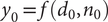 $ {y}_0=f\left({d}_0,{n}_0\right) $
. If the
$ {y}_0=f\left({d}_0,{n}_0\right) $
. If the
 $ {y}_0 $
value is not bounded by the Hessian terms, there is a nonmonotonic quadratic nature to the response
$ {y}_0 $
value is not bounded by the Hessian terms, there is a nonmonotonic quadratic nature to the response
 $ f $
. This is well known in traditional factorial experimentation (Montgomery Reference Montgomery2017) and applies equally here. So instead of just four Hessian points to evaluate
$ f $
. This is well known in traditional factorial experimentation (Montgomery Reference Montgomery2017) and applies equally here. So instead of just four Hessian points to evaluate
 $ f $
, one should also include the nominal value point and ensure the nominal falls within the bounds of the Hessian points. This is shown as interaction plots in Figure 3.
$ f $
, one should also include the nominal value point and ensure the nominal falls within the bounds of the Hessian points. This is shown as interaction plots in Figure 3.

Figure 3. Non-monotonic interactions requiring backward and forward differences.
When the nominal value falls outside of the Hessian term response values, the central differencing domain must be split into two regimes, the upper and lower range on either
 $ {d}^j $
,
$ {d}^j $
,
 $ {n}^i $
or both. Typically, an engineer expects quadratic behaviour of certain variables and whether the cause is from the
$ {n}^i $
or both. Typically, an engineer expects quadratic behaviour of certain variables and whether the cause is from the
 $ {d}^j $
,
$ {d}^j $
,
 $ {n}^i $
or both can be self-stated a priori. Whichever it is, the four central differenced Hessian points must be augmented with two more axial points on that variable. Then backward differencing is used between the negative points and nominal points, and forward differencing on the nominal points and positive points. This results in two Hessian terms that can be considered for the impact of a design change. If the source of the quadratic behaviour as
$ {n}^i $
or both can be self-stated a priori. Whichever it is, the four central differenced Hessian points must be augmented with two more axial points on that variable. Then backward differencing is used between the negative points and nominal points, and forward differencing on the nominal points and positive points. This results in two Hessian terms that can be considered for the impact of a design change. If the source of the quadratic behaviour as
 $ {d}^j $
or
$ {d}^j $
or
 $ {n}^i $
cannot be self-stated, then the axis points on both will need to be evaluated, at the expense of four additional function evaluations.
$ {n}^i $
cannot be self-stated, then the axis points on both will need to be evaluated, at the expense of four additional function evaluations.
Overall, the central differencing evaluation of the Hessian ought first be used for bilateral problems, as it is more accurate about a nominal point. In this initial calculation, it should be checked against the nominal point for quadratic behaviour of the response. If the nominal point is not bounded by the central difference points, then the central difference Hessian is incorrect, Figure 3a. In such cases, the central difference domain needs to be split to include the two nominal axial points and then two Hessian terms computed, the upper and lower. The two results are then the different impact in variability with a positive or negative change for quadratic response design variables, or the different impact in variability of a design change on the upper and lower variations for quadratic response noise variables.
2.5. Jacobian mean shift term
The design changes suggested by the above Hessian calculations can result not only in variance reduction, but also in mean shift. Often this is undesirable, as the nominal performance
 $ \overline{y} $
is targeted. In this case, the Jacobian can similarly be used to compute means shifts, to shift the mean back to target while reducing the variation.
$ \overline{y} $
is targeted. In this case, the Jacobian can similarly be used to compute means shifts, to shift the mean back to target while reducing the variation.
Again, consider a Taylor Series expansion of the response at the current nominal (
 $ {d}_0 $
,
$ {d}_0 $
,
 $ {n}_0 $
),
$ {n}_0 $
),
 $$ y=f\left(d,n\right)={y}_0+\frac{\partial f}{\partial n}\left(n-{n}_0\right)+\frac{\partial f}{\partial d}\left(d-{d}_0\right). $$
When changing a design variable
 $ {d}^j $
to reduce variation, the Jacobian can indicate how much the mean will shift. Further, we can use a variable
$ {d}^j $
to reduce variation, the Jacobian can indicate how much the mean will shift. Further, we can use a variable
 $ {d}^j $
which has no influence on the Hessian to shift back the mean to its original value. Here,
$ {d}^j $
which has no influence on the Hessian to shift back the mean to its original value. Here,
 $$ {J}^j=\frac{1}{2}\frac{\partial f}{\partial {d}^j}\approx \frac{\sum_{d^j={d}_{+}}y}{N}-\frac{\sum_{d^j={d}_{-}}y}{N}, $$
where
 $ N $
is the number of runs done in the Hessian analysis, where half are at
$ N $
is the number of runs done in the Hessian analysis, where half are at
 $ {d}_{+} $
and half are at
$ {d}_{+} $
and half are at
 $ {d}_{-} $
. Reference Arena, Leonard, Murray and YounossiEquation (2) computes the half-effect of moving from the nominal center to either of the end points
$ {d}_{-} $
. Reference Arena, Leonard, Murray and YounossiEquation (2) computes the half-effect of moving from the nominal center to either of the end points
 $ {d}_{+} $
or
$ {d}_{+} $
or
 $ {d}_{-} $
.
$ {d}_{-} $
.
The overall change in response mean is then approximately a linear summation of the design variable changes,
 $$ \Delta \overline{p}(d)=\sum_j\left({J}^j\right)\Delta {d}^j, $$
where again
 $ \Delta {d}^j $
is the amount of change to
$ \Delta {d}^j $
is the amount of change to
 $ {d}^j $
in a new design configuration considered.
$ {d}^j $
in a new design configuration considered.
In combination with the variation reduction as computed by Equation (13) and the mean shift as computed by Equation (21), one can select design variable changes to reduce the variation while constraining the mean to a target. Design variables that reduce variation can be determined and set using Equation (13). The associated mean shift from those changes can be computed using Equation (21), and different design variables changed to shift the mean back to the desired target. In this way, variation can be minimised subject to a constrained mean. Furthermore, the reasons for the variation reduction are made explicit. The identified design variables that can reduce the impact of identified noise variables will be clear, rather than a black box experimental optimisation approach.
3. Stirling engine design example
In previous work, (Otto & Sanchez Reference Otto and Sanchez2019; Otto, Wang, & Uyan Reference Otto, Wang and Uyan2019) workflows were developed applying UQ and GSA methods to identify root causes of manufacturing quality problems and in Sanchez, Björkman, & Otto (Reference Sanchez, Björkman and Otto2020), a workflow was developed using design of experiments to achieve robustness improvement, and in Sanchez Mosqueda & Otto (Reference Sanchez Mosqueda and Otto2021), we introduced using Hessian terms. Here, we build on these previous works to now consider the greater insight and fewer runs offered by the Hessian approach and in conjunction with compounded variables.
3.1. Stirling engine case study
In these previous works, we introduced the example of a miniature Stirling engine case study. At Aalto University students fabricated, assembled and tested Stirling engines as part of the senior level machine design course. Students measured the speed at which the crank shaft rotates when there is no torque load applied, the no-load speed. The no-load speed tests demonstrated 25% variation in speed across the fabricated engines, due to variations in fabrication. This outcome exposed the high sensitivity of the Stirling engine to manufacturing and assembly variations. Here, we follow the approach of Figure 1 to explore if the variability of the design could be reduced through parametric design changes. We also compare the insights and speed of the approach with traditional robustness optimisation.
The geometric input variables of the Stirling engine are shown in Figure 4. There is a hot side cylinder heated externally with a transfer piston that exchanges air from the hot side to the cold side. There is a cold-side power cylinder and piston that extracts mechanical power from the air as it expands and contracts due to the transfer piston movement. The pistons are connected by a shaft with an offset angle of 90°.

Figure 4. Stirling Engine Geometry.
3.2. Step 1 UQ/GSA
Following Figure 1, the first step of the workflow is to quantify the uncertainty at the original design and determine noise variable contributors through a GSA. We used a toolchain developed in Otto & Sanchez (Reference Otto and Sanchez2019), which creates UQ samples using Latin Hypercube sampling and runs an external Matlab code (Sanchez Mosqueda & Otto Reference Sanchez Mosqueda and Otto2021) to compute the engine power at each point. Executing the UQ also requires a number of evaluations, independent of the evaluations needed to compute the robust design variance reduction discussed here. We take the approach discussed in Section 2.1, where we start with a small sample and compute the UQ and also fit a surrogate model to the UQ sample points for use with the GSA analysis. We sequentially increase the UQ sample size until surrogate model fits well. In the Stirling engine case, this required 40 samples to fit a distribution and surrogate model with under 2% error (
 $ {r}^2 $
of 98%). Figure 5 shows the histogram of the thermodynamic power response. The average power is 1.63 W with a standard deviation of ±0.09 W.
$ {r}^2 $
of 98%). Figure 5 shows the histogram of the thermodynamic power response. The average power is 1.63 W with a standard deviation of ±0.09 W.

Figure 5. Uncertainty of engine powerat the nominal design.
A surrogate model is fit through the UQ sample points for use in the GSA. A vast selection of machine learning methods are available in the Python code library scikit-learn (Ureili Reference Ureili2010) and used in our toolchain. Here, we applied Kernel Ridge Regression with a cross-validated grid search routine implemented for hyperparameter tuning. The resulting surrogate model matched the simulation with r 2 = 0.98 on the test data. With this surrogate model, Saltelli samples were generated and Sobol indices computed. Figure 6 shows the resulting variance contribution to the power variability by each noise variable alone and by higher-order interactions, where all higher-order interactions among the small noise variations were negligible.

Figure 6. Sobol sensitivity analysisof the power variability at the nominal design.
The GSA indicates variation of the cold-side clearance volume, outer transfer cylinder diameter, swept volume of the expansion piston and swept volume of the compression piston as the largest contributors to power variability.
3.3. Unconstrained minimisation
The second step in the workflow is to construct Hessian cross terms to quickly compute the effect of any design change on reducing contributions to response variability. First, design variables are proposed. We make use of input volumetric variables compounded from dimensional geometry of the engine. Clearance and swept volumes from compression and expansion sides
 $ \left({V}_{clc},{V}_{swc},{V}_{clh}\hskip0.24em \mathrm{and}\;{V}_{swh}\right) $
were selected as design variables
$ \left({V}_{clc},{V}_{swc},{V}_{clh}\hskip0.24em \mathrm{and}\;{V}_{swh}\right) $
were selected as design variables
 $ {d}^j $
. From the GSA the largest contributors to engine power variability were
$ {d}^j $
. From the GSA the largest contributors to engine power variability were
 $ \left({\Delta V}_{clc},\Delta {V}_{swc},{\Delta V}_{swh}\hskip0.24em \mathrm{and}\;\Delta {d}_{out}\right) $
and so used as noise variables
$ \left({\Delta V}_{clc},\Delta {V}_{swc},{\Delta V}_{swh}\hskip0.24em \mathrm{and}\;\Delta {d}_{out}\right) $
and so used as noise variables
 $ {n}^i $
. Then
$ {n}^i $
. Then
 $ \pm 4\sigma $
ranges were defined for the noise variables and a reasonable
$ \pm 4\sigma $
ranges were defined for the noise variables and a reasonable
 $ \pm 20\% $
range of optimisation for the design variables.
$ \pm 20\% $
range of optimisation for the design variables.
The Hessian cross terms are constructed in terms of the 4 noise variables and 4 design variables, 16 combinations requiring a total of 64 runs. Table 1 shows how making a design variable increase by +20% changes the
 $ \pm 4{\sigma}_i $
thermodynamic power range (W), using Equation (10). It shows, for example, that when changing the design variable
$ \pm 4{\sigma}_i $
thermodynamic power range (W), using Equation (10). It shows, for example, that when changing the design variable
 $ {V}_{clc} $
+20%, the variability in thermodynamic power due to the manufacturing variation
$ {V}_{clc} $
+20%, the variability in thermodynamic power due to the manufacturing variation
 $ \Delta {V}_{clc} $
will go down by ±0.01 W, a significant reduction of the ±0.09 W standard deviation. Table 1 also shows that the contribution to thermodynamic power variation due to
$ \Delta {V}_{clc} $
will go down by ±0.01 W, a significant reduction of the ±0.09 W standard deviation. Table 1 also shows that the contribution to thermodynamic power variation due to
 $ \Delta {V}_{swc} $
and
$ \Delta {V}_{swc} $
and
 $ \Delta {V}_{swh} $
are not significantly affected by any of the proposed design changes, since rows 2 and 3 all have small terms.
$ \Delta {V}_{swh} $
are not significantly affected by any of the proposed design changes, since rows 2 and 3 all have small terms.
Table 1. Twenty percent increase design variable change impact on standard deviation contributions

Improved understanding can be provided by normalising the results of Table 1 into percentages as Sobol indices, using Equation (12). Table 2 shows the change to a noise variable’s Sobol index
 $ {S}_i $
by changing a design variable by +20%. Note these are the additive increments to each main effect Sobol index, they are not multipliers on the total variance. Therefore, they do not show how much the total variance is percentage reduced. Rather, Equation (13) is needed, with results shown in Table 3.
$ {S}_i $
by changing a design variable by +20%. Note these are the additive increments to each main effect Sobol index, they are not multipliers on the total variance. Therefore, they do not show how much the total variance is percentage reduced. Rather, Equation (13) is needed, with results shown in Table 3.
Table 2. Twenty percent increase design change interaction impact on Sobol indices

Table 3. Twenty percent increase design change interaction impact on variance percent

The interaction impact on response variance indicates making an increase of 20% to the nominal
 $ {V}_{clc} $
will reduce the contribution of
$ {V}_{clc} $
will reduce the contribution of
 $ \Delta {V}_{clc} $
variance by 21%, whereas making a decrease of 20% to the nominal
$ \Delta {V}_{clc} $
variance by 21%, whereas making a decrease of 20% to the nominal
 $ {V}_{swh} $
will reduce the contribution of
$ {V}_{swh} $
will reduce the contribution of
 $ \Delta {V}_{clc} $
variance by 22%. Overall, Equation (13) indicates that in combination making the two design changes together will show a 39% power variance reduction due to the input noise variation on
$ \Delta {V}_{clc} $
variance by 22%. Overall, Equation (13) indicates that in combination making the two design changes together will show a 39% power variance reduction due to the input noise variation on
 $ \Delta {V}_{clc} $
alone, and a 43% reduction due to all four input noise variations. Note that the design changes had little impact on the thermodynamic power variation caused by
$ \Delta {V}_{clc} $
alone, and a 43% reduction due to all four input noise variations. Note that the design changes had little impact on the thermodynamic power variation caused by
 $ \Delta {V}_{swc} $
or
$ \Delta {V}_{swc} $
or
 $ \Delta {V}_{swh} $
input noise variations, rows 2 and 3 are small. This Hessian approach provides insight into how and why design changes reduce response variation.
$ \Delta {V}_{swh} $
input noise variations, rows 2 and 3 are small. This Hessian approach provides insight into how and why design changes reduce response variation.
Figure 7 shows the Hessian calculation results graphically as a matrix plot. Each column is a design variable and each row is a noise variable. Each plot therefore has a design variable as the x-axis and thermodynamic power as the y-axis, and two lines of the response with the noise variable high and low. Therefore, parallel lines indicate no impact of a design change over a noise contribution, and highly nonparallel lines show a strong ability of the design variable to reduce the impact of the noise variable. Design variable values are sought which bring the two lines together. The upper left plot indicates a large change to design variable
 $ {V}_{clc} $
will reduce
$ {V}_{clc} $
will reduce
 $ \Delta {V}_{clc} $
variability contribution to power. The upper second plot indicates a large change to design variable
$ \Delta {V}_{clc} $
variability contribution to power. The upper second plot indicates a large change to design variable
 $ {V}_{swc} $
will have no impact on the
$ {V}_{swc} $
will have no impact on the
 $ \Delta {V}_{clc} $
variability contribution to power. Overall, the plots show design variables
$ \Delta {V}_{clc} $
variability contribution to power. Overall, the plots show design variables
 $ {V}_{clc} $
and
$ {V}_{clc} $
and
 $ {V}_{swh} $
can reduce variation (bring the two lines closer together), that
$ {V}_{swh} $
can reduce variation (bring the two lines closer together), that
 $ {V}_{clc} $
,
$ {V}_{clc} $
,
 $ {V}_{swc} $
and
$ {V}_{swc} $
and
 $ {V}_{swh} $
can shift the mean (lines have non-zero slope) and that
$ {V}_{swh} $
can shift the mean (lines have non-zero slope) and that
 $ {V}_{clh} $
affects neither the mean nor variance (lines are flat and parallel).
$ {V}_{clh} $
affects neither the mean nor variance (lines are flat and parallel).

Figure 7. Interaction Hessian graphs.
Having identified new design values for
 $ {V}_{clc} $
and
$ {V}_{clc} $
and
 $ {V}_{swh} $
, we proceed to compute UQ/GSA at the new design. Figure 8 shows the uncertainty of engine power at new design configuration. The standard deviation went down from ±0.09 to ±0.06 W, indicating a (squared) variance reduction by 49%, similar as the Hessian reduction predicted 43% given by Equation (13).
$ {V}_{swh} $
, we proceed to compute UQ/GSA at the new design. Figure 8 shows the uncertainty of engine power at new design configuration. The standard deviation went down from ±0.09 to ±0.06 W, indicating a (squared) variance reduction by 49%, similar as the Hessian reduction predicted 43% given by Equation (13).

Figure 8. Uncertainty change of engine power at the new unconstrained configuration.
Next, we continue with Step 4 of the workflow and recompute a GSA to confirm total response variance contributions. Figure 9 shows how the power variance was reduced, and that it was due to the
 $ \Delta {V}_{clc} $
noise variable Sobol index being reduced by 4.5% which is close with that shown previously in Table 2 of 6%. This is as expected from the Hessian analysis which showed the design changes only mitigate the impact of the
$ \Delta {V}_{clc} $
noise variable Sobol index being reduced by 4.5% which is close with that shown previously in Table 2 of 6%. This is as expected from the Hessian analysis which showed the design changes only mitigate the impact of the
 $ \Delta {V}_{clc} $
noise contribution.
$ \Delta {V}_{clc} $
noise contribution.

Figure 9. Sobol sensitivity analysis of the model computed power variability at the new design.
3.4. Constrained variation reduction
Although a 49% reduction on variance was achieved at the new design, the mean power was shifted down to 1.21 W from 1.64 W. To constrain the mean power from shifting, the Jacobian terms can be used to shift back the mean closer to the mean at nominal design. We therefore revert back to Step 2 of the workflow and following Equation (21), we computed the change in power due to changes in design variable
 $ {d}^j $
. This is shown in Table 4. The values indicate the average power would shift down by (−0.31–0.6)/2 = 0.45 W with the 20% design changes to
$ {d}^j $
. This is shown in Table 4. The values indicate the average power would shift down by (−0.31–0.6)/2 = 0.45 W with the 20% design changes to
 $ {V}_{clc} $
and
$ {V}_{clc} $
and
 $ {V}_{swh} $
, which agrees with the observed shift to 1.21 W.
$ {V}_{swh} $
, which agrees with the observed shift to 1.21 W.
Table 4. Normalised Jacobian terms for mean shift from nominal

Similar to Figure 6, one can create variable plots of the power response values versus each design variable. Figure 10 shows how average power changes when each design variable changes by ±20%. The Hessian calculation showed that design variables
 $ {V}_{clc} $
,
$ {V}_{clc} $
,
 $ {V}_{swc} $
and
$ {V}_{swc} $
and
 $ {V}_{swh} $
influence on variance response, whereas design variable
$ {V}_{swh} $
influence on variance response, whereas design variable
 $ {V}_{clh} $
does not. Changing design variables
$ {V}_{clh} $
does not. Changing design variables
 $ {V}_{clc} $
by +20% and
$ {V}_{clc} $
by +20% and
 $ {V}_{swh} $
, by −20%, as suggested by the Hessian calculations, will cause not only a reduction in response variance but also a shift in response mean. Hence,
$ {V}_{swh} $
, by −20%, as suggested by the Hessian calculations, will cause not only a reduction in response variance but also a shift in response mean. Hence,
 $ {V}_{swc} $
and
$ {V}_{swc} $
and
 $ {V}_{clh} $
can be changed to compensate and shift back average power.
$ {V}_{clh} $
can be changed to compensate and shift back average power.

Figure 10. Average Power Changes with design variable changes.
3.5. Constrained optimisation using Hessians and Jacobian formulas
The Step 4 in the workflow is to solve an optimisation to calculate the amount of change required for each design variable to produce the same response as the nominal design variables but with a reduced standard deviation. The objective function was set to minimise variation and constraints were added to maintain an average power change of zero and a design space from −20% to 20%.
Equation (13) for the power variance and the Jacobian derived Equation (21) can be simultaneously solved in a constrained optimisation
 $$ {\displaystyle \begin{array}{l}\mathrm{Find}\hskip0.5em {d}_{\ast }=\arg \hskip0.5em \underset{d}{\min }{\sigma}_p^2\\ {}\mathrm{subject}\hskip0.5em \mathrm{to}\hskip0.5em \overline{p}-1.6\ge 0\\ {}0.8{d}_{i0}\le {d}^i\le 1.2{d}_{i0}\end{array}} $$
The result is a new design configuration shown in Table 5, along with the Hessian predicted change in variance and Jacobian predicted change in average power. The solution showed an expected 13% reduction in variance with no change in mean. Notice the solution drove
 $ {V}_{clc} $
to the largest +20% given the Sij coefficients, but it did not drive
$ {V}_{clc} $
to the largest +20% given the Sij coefficients, but it did not drive
 $ {V}_{swh} $
to the smallest −20% since that is not possible with the constraint on the allowed mean shift. The terms
$ {V}_{swh} $
to the smallest −20% since that is not possible with the constraint on the allowed mean shift. The terms
 $ {V}_{swc} $
and
$ {V}_{swc} $
and
 $ {V}_{clh} $
can shift the mean but do not change the variation much, accounting for approximately +0.25 W increase in mean. This restricts the extent of the
$ {V}_{clh} $
can shift the mean but do not change the variation much, accounting for approximately +0.25 W increase in mean. This restricts the extent of the
 $ {V}_{swh} $
shift.
$ {V}_{swh} $
shift.
Table 5. New design configuration

3.6. UQ at the new design
To confirm a variation reduction and a mean power similar to the nominal design, we proceed with Step 5 to quantify uncertainty at the new design. Figure 11 shows the standard deviation and mean power of the new design. The new design configuration shows a standard deviation of ±0.08 W and an average power of 1.64 W. This result shows a (squared) reduction of 20% in variance and no change in average power in relation to nominal design. This actual is in agreement with the variation reduction predicted with the Hessian terms of 13%.

Figure 11. Uncertainty change of engine power at the new constrained design configuration.
4. Compounded variables
Equation (9) computed the Hessian terms in four runs for each combination of significant noise factor and each hypothesised design variable. The complexity of this approach grows as four times N, the number of design variables times M, the number of noise variables. While better than other approaches, 4 NM can still be prohibitive. However, if one has engineering knowledge of the slope of the noise variables contribution to the response, they can be compounded (Taguchi & Taguchi Reference Taguchi and Taguchi2000). Further, a similar compounding approach can be taken with the design variables.
4.1. Compounded noise variables
Consider a noise variable with positive slope in the response, and a second with negative slope. Then instead of executing runs over both noise factors with the design variables, a single compound noise variable set can be used where each is varied simultaneously and, in this case, in opposite direction. In the limit of compounding all noise factors, this will reduce the number of evaluations from 4 NM to 4 N.
As an example, in the Stirling engine example, the noise variables
 $ \Delta {V}_{clc} $
had negative slope whereas
$ \Delta {V}_{clc} $
had negative slope whereas
 $ {\Delta V}_{swc} $
and
$ {\Delta V}_{swc} $
and
 $ \Delta d $
had positive slope and
$ \Delta d $
had positive slope and
 $ {\Delta V}_{swh} $
had zero slope. Therefore, a single compound noise variable could be used composed of
$ {\Delta V}_{swh} $
had zero slope. Therefore, a single compound noise variable could be used composed of
 $ n=\left({\Delta V}_{clc},\Delta {V}_{swc},{\Delta V}_{swh},\Delta {d}_{out}\right) $
and the two values to use are
$ n=\left({\Delta V}_{clc},\Delta {V}_{swc},{\Delta V}_{swh},\Delta {d}_{out}\right) $
and the two values to use are
 $ {n}_{-}=\left(+,-,0,-\right) $
and
$ {n}_{-}=\left(+,-,0,-\right) $
and
 $ {n}_{+}=\left(-,+,0,+\right) $
.
$ {n}_{+}=\left(-,+,0,+\right) $
.
With compound noise variables, the width between the upper and lower limit responses grows with the number of variables. Therefore, similar to previously, to keep the result at a fixed number of standard deviations the computed compound variable Hessian terms need to be scaled by the square root of the number of noise variables compounded,
 $$ {H}_{n,j}=\frac{1}{\sqrt{M}}{H}^{ij}, $$
where here
 $ {H}^{ij} $
is as computed using Equation (9) with a single but compounded noise variable.
$ {H}^{ij} $
is as computed using Equation (9) with a single but compounded noise variable.
The results of this compounding are shown in Table 6, and show the same results as before, larger
 $ {V}_{clc} $
and smaller
$ {V}_{clc} $
and smaller
 $ {V}_{swh} $
reduce power variability. This here is computed with less runs (16 runs), 25% run-time of the noncompounded (64 runs).
$ {V}_{swh} $
reduce power variability. This here is computed with less runs (16 runs), 25% run-time of the noncompounded (64 runs).
Table 6. Compound noise variable impact on variance

In the workflow of Figure 1, compounding noise variables is an easy simplification to make, since in the first step a UQ is performed and the results can be plotted against each noise variable and the nominal slope direction determined.
On the other hand, while reducing calculations, the noise factor compounding also reduces information provided. It is not clearly highlighted which Sobol index is being reduced, and therefore which noise factor contribution in the compounded variable is being reduced. While it is highlighted the response variance is reduced, it is not highlighted that the reductions are contributions from noise factors
 $ {\Delta V}_{clc} $
and
$ {\Delta V}_{clc} $
and
 $ \Delta {d}_{out} $
being reduced. It is not highlighted that the contributions from noise factors
$ \Delta {d}_{out} $
being reduced. It is not highlighted that the contributions from noise factors
 $ \Delta {V}_{swc} $
or
$ \Delta {V}_{swc} $
or
 $ {\Delta V}_{swh} $
are negligibly changed. Overall, compounding is more efficient, but at the expense of less engineering insight on how the design changes are impacting which noise factor contributions.
$ {\Delta V}_{swh} $
are negligibly changed. Overall, compounding is more efficient, but at the expense of less engineering insight on how the design changes are impacting which noise factor contributions.
4.2. Compounded design variables
Similar to noise variables, design variables can also be compounded. Unlike with noise variables, though, doing so requires a priori engineering knowledge of how the response changes with design variable changes. As with noise factors, if two design variables have the same slope, they can be varied the same, and if they have opposite slopes they can be varied in opposition.
For example, with the Stirling engine we may have knowledge that decreases in the cold side volume
 $ {V}_{clc} $
reduces power, and increasing the swept volume
$ {V}_{clc} $
reduces power, and increasing the swept volume
 $ {V}_{swh} $
increases power. These could be varied as a single design variable
$ {V}_{swh} $
increases power. These could be varied as a single design variable
 $ d=\left({V}_{clc},{V}_{swh}\right) $
. Then the compounded values would be
$ d=\left({V}_{clc},{V}_{swh}\right) $
. Then the compounded values would be
 $ {d}_{-}=\left(+,-\right) $
and
$ {d}_{-}=\left(+,-\right) $
and
 $ {d}_{+}=\left(-.+\right) $
. The results of this are shown in Table 7, larger
$ {d}_{+}=\left(-.+\right) $
. The results of this are shown in Table 7, larger
 $ {V}_{clc} $
and smaller
$ {V}_{clc} $
and smaller
 $ {V}_{swh} $
reduce power variability, and impact the
$ {V}_{swh} $
reduce power variability, and impact the
 $ {\Delta V}_{clc} $
and
$ {\Delta V}_{clc} $
and
 $ \Delta {d}_{out} $
noise contributions most. This is similar to as computed before but with less runs, (16 runs), 25% run-time of the noncompounded (64 runs).
$ \Delta {d}_{out} $
noise contributions most. This is similar to as computed before but with less runs, (16 runs), 25% run-time of the noncompounded (64 runs).
Table 7. Compound design variable impact on variance

In the workflow of Figure 1, there are no steps to provide any indication on how to compound design variables. Without a-priori knowledge, one factor at a time runs could be done (axial points), but at added expense of more evaluations.
Finally, notice that if it were possible to be equipped with a priori knowledge of both design and noise variable directionality then all variables could be compounded, on both the design and noise variables. This reduces the entire 4 NM set of runs down to a mere four runs. The sign of the one term of Equation (9) would indicate which direction to change the compound design variable to reduce variability from the compounded noise variables.
For example, with the Stirling engine, compounding the noise variables into a single compound noise variable and compounding the two
 $ {V}_{clc} $
and
$ {V}_{clc} $
and
 $ {V}_{swh} $
design variables into a single compound design variable, the results of this are shown in Table 8, and compute most compactly the same as before. Making a 20% change to the two design variables (
$ {V}_{swh} $
design variables into a single compound design variable, the results of this are shown in Table 8, and compute most compactly the same as before. Making a 20% change to the two design variables (
 $ {V}_{clc} $
larger and
$ {V}_{clc} $
larger and
 $ {V}_{swh} $
smaller) reduces the variation from the four noise factors by 46%. This is similar to as computed earlier but with much less evaluations (4 runs), 6% run time compared to the non-compounded (64 runs).
$ {V}_{swh} $
smaller) reduces the variation from the four noise factors by 46%. This is similar to as computed earlier but with much less evaluations (4 runs), 6% run time compared to the non-compounded (64 runs).
Table 8. Compound design variable impact on compound noise variance

While one cannot compute constrained variation reduction of Equation (22), this compounded variable Hessian approach is nonetheless substantially more efficient in comparison to many alternative optimisation formulations with extensive computational requirements. It does, however, require engineering knowledge of how the noise and design variables change the response. In comparison to the rich literature on probabilistic optimisation methods and robust design of experiments, it demonstrates a substantial limit case of computational simplifications that are possible in solving unconstrained variability minimisation. All other known probabilistic optimisation methods apply more than four evaluations.
5. Discussion: comparison with uncertainty optimisation
The approach successfully computed a new design with less variability, and successfully found a new design with less variability constrained to target the nominal average power. Further, the approach made use of only 64 runs to quantify the individual impact potential of 4 design variable changes on the contributions of 4 significantly contributing noise variables. Insight was provided that only two of the four most contributing noise variables can be impacted by the proposed design changes.
The results can be compared against a more comprehensive exploration of the design and noise space using robust optimisation. In earlier work (Sanchez, Björkman, & Otto Reference Sanchez, Björkman and Otto2020) an RDM UQ minimisation approach was undertaken using traditional surrogate-model probabilistic optimisation (Chen et al. Reference Chen, Allen, Tsui and Mistree1996; Fang, Li, & Sudjianto Reference Fang, Li and Sudjianto2005; Allen et al. Reference Allen, Seepersad, Choi and Mistree2006; Chen, Jin, & Sudjianto Reference Chen, Jin and Sudjianto2006; Jiang, Chen, & German Reference Jiang, Chen and German2016). One hundred sample points were used over the design space and 40 sample points used in a UQ to cover the noise space. This resulted in 4000 runs total. At each design space point, a 40-point UQ was executed and the mean and variance of the power computed. The two statistics were computed at each sample point in the design space, and surrogate models were fit. Then a Pareto optimisation was solved to show the best combinations of surrogate model estimated mean and variance of power over the ±20% domain of the design variables. This is shown in Figure 12, where the red line represents all computed Pareto optimal solutions between minimising variance and maximising the nominal power.

Figure 12. Pareto optimal solutions and Hessian results.
As can be seen, the Hessian approach solved the problem well despite using much less runs than either a traditional RDM design of experiments or optimisation approach. The unconstrained Hessian solution solved to the same design variable outcomes as the probabilistic optimisation result. Also shown is the unconstrained solution when varying only the most significant two design variables by 20%, as found with only the Hessian terms. Finally, the constrained solution found by the Hessian plus Jacobian approach solved to the same design variable combination solution as the full probabilistic optimisation approach. The Hessian approach is approximate, it relies on a single-numerical derivatives and so finding the optimised results should not be expected in all cases. However, the approach will positively identify useful design variables to change to reduce response variability.
The probabilistic optimisation approach compared here is but one of many in the rich literature of robust design optimisation. The design of experiment approach (Taguchi Reference Taguchi1986; Phadke Reference Phadke1989; Taguchi & Taguchi Reference Taguchi and Taguchi2000), surrogate modelling approaches to robust design (Jin, Chen, & Simpson Reference Jin, Chen and Simpson2001; Chen, Jin, & Sudjianto Reference Chen, Jin and Sudjianto2006) and optimisation of quantified probabilistic uncertainty (Allen et al. Reference Allen, Seepersad, Choi and Mistree2006) would all produce the same optimised results as shown. The comparison of sample based methods with purely optimisation formulations such as most-probable-point reliability based design has been done elsewhere (Du, Sudjianto, & Chen Reference Du, Sudjianto and Chen2004). Optimising quantified uncertainty has least approximations at the expense of computational burden; surrogate modelling introduces approximations but provides significant reductions in calculations. Design of experiments simplifies the calculations even further to regression models, with further approximation. We here simplify even further to consideration of merely the Hessian terms, at significant reduced calculations but also increased approximation.
As such, the Hessian approach here cannot determine an optimal solution when the search function has multiple optima; the previously mentioned methods ought be considered. However, when a design engineer must compute the UQ/GSA for verification purposes, this approach also allows a rapid manner to identify design variables to consider and their direction of change to reduce response variance.
Overall, we find the Hessian approach to variation reduction exploration intuitive and insightful. It allows one to quickly screen design variables for their ability to reduce response variance and with a clear indicator of how the design variable is doing this variance reduction, in terms of interaction contributions of significant noise variables.
6. Conclusion
The traditional and well-researched RDM has a wealth of research and techniques to compute design changes that reduce performance variability. Such optimisation of uncertainty can sometimes become computationally difficult, whether through direct optimisation of quantified uncertainty as an objective function or through Taguchi type robust design of experiments.
Here, we made use of the more easily computed Hessian matrix cross terms between the variance-contributing noise variables and the variables of any proposed design changes. Design variable changes with large Hessian terms against noise variables are design changes that can reduce variability. Further, the Jacobian terms of these design changes can indicate which design variables can shift the mean response, to maintain a desired performance target. Using a combination of the more easily computed Hessian and Jacobian terms, design changes can be proposed to reduce variability while maintaining a targeted nominal.
We relate here the Hessian predicted reductions to the associated reductions in Sobol indices that indicate the percentage contribution of noise variables. We also relate these to the percentage reduction expected in the response variance. This allows for rapid interpretation of the impact of different design variable changes in a modern UQ/GSA optimisation workflow.
The most basic industrial RDM workflow is to estimate the variance of a design concept, propose design changes and then estimate the reduced variance after making the design changes. We applied this workflow to computational practice through UQ and GSA as a first and last step. An example was shown on a Stirling engine design where the impact of the top three variance-contributing tolerances were studied for variation reduction. The approach quickly identified two significant design variables, and found a new design with 20% less variance and no change in nominal average power. Overall, we find this Hessian-based RDM approach useful for classes of problems with high-computational burdens.
Acknowledgements
This work was made possible with support from the Academy of Finland, Project Number 310252.
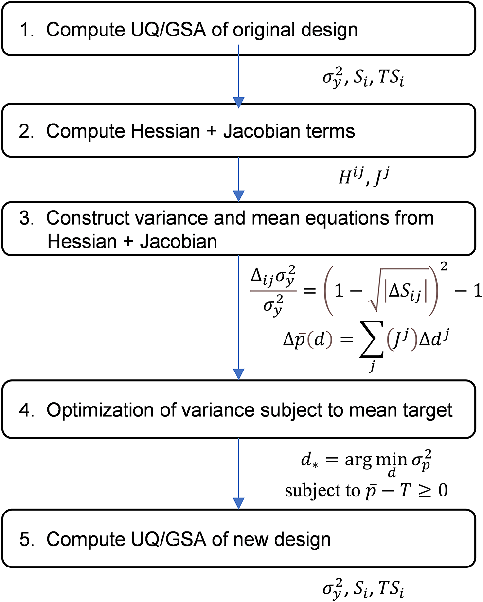


 Open access