


1. Introduction
Models of the gravity-driven motion of a viscous liquid have been used to describe and interpret a range of geophysical phenomena, including lava flows, magma chambers and glaciers (Huppert Reference Huppert1986). The classical model of the spreading of a viscous liquid on a horizontal or inclined plane (Huppert Reference Huppert1982; Lister Reference Lister1992), has been extended to account for many geophysically relevant features, including cooling (Lyman, Kerr & Griffiths Reference Lyman, Kerr and Griffiths2005), a yield stress (Balmforth, Craster & Sassi Reference Balmforth, Craster and Sassi2002), and the effect of a second overlying fluid that can deform during the motion (Kowal & Worster Reference Kowal and Worster2015).
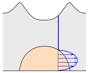
Here, we analyse the gravity-driven spreading of a viscous liquid at the base of a granular mush of finite thickness, which is transported and deformed by the viscous motion; see figure 1. This problem has fundamental fluid dynamical interest as a novel two-fluid gravity current of materials with distinct rheological properties. However, the study is also motivated by the formation of massive sulphide ores in magmatic systems (Hinton & Slim Reference Hinton and Slim2023), and has a secondary application to layered mafic intrusions (Maier, Barnes & Groves Reference Maier, Barnes and Groves2013; Liu et al. Reference Liu, Zhou, Wang, Xing and Gao2014).

Figure 1. Schematic diagram illustrating two-dimensional gravity-driven flow of a viscous liquid beneath a granular mush. The red lines and arrows show a typical flow profile.
Massive sulphide ore deposits form small portions of basaltic magmatic intrusions within the Earth's crust. They are thought to have formed from metal-sulphide-rich liquid droplets within the dominant silicate melt, coalescing and depositing in particular parts of the magmatic plumbing system (Robertson, Barnes & Le Vaillant Reference Robertson, Barnes and Le Vaillant2016). Transport of the sulphide-rich liquid occurs as the system cools, and hence involves interaction with a mush of silicate melt and silicate crystals. Of particular interest is the final location of this sulphide-rich liquid, thus understanding the transport within the crystal-rich environment is key.
To capture the dominant processes associated with a coalesced volume of dense sulphide-rich liquid interacting with a mixture of silicate crystals and liquid, we model the system as a two-dimensional shallow isothermal flow. The sulphide-rich liquid is represented by a relatively dense viscous liquid, whilst the silicate crystals within the silicate liquid are modelled by a continuum granular mush (see figure 1). Importantly, the two liquids are different, and the silicate crystals within the magma are non-wetting to the sulphide liquid (Mungall & Su Reference Mungall and Su2005). Hence we assume that there is no interpenetration across the sharp interface between the viscous liquid and the granular mush. The granular mush is assumed to obey a  $\mu (I)$-rheology, which has been shown to capture accurately many experimental features of granular flows (GDR-MiDi 2004; Gray & Edwards Reference Gray and Edwards2014).
Recently, Hinton & Slim (Reference Hinton and Slim2023) investigated the spreading of a viscous gravity current atop a dense granular mush. This was motivated by the same magmatic system but with the sulphide liquid remaining atop the silicate mush and unable to penetrate downwards owing to the capillary entry pressure. They found that the viscous liquid initially erodes the underlying granular mush into levees. Subsequently, the top part of the levee is pushed outwards by the viscous liquid, with the remnants of the levees trapping a significant fraction of the liquid.
In the present work, we consider the opposite configuration, with the relatively dense viscous liquid lying at the bottom of the granular mush. The lower boundary (at  $\hat {z}=0$) is impermeable and corresponds to the host country rock bounding the magma chamber. Both configurations are geologically relevant as the dense liquid sulphide may penetrate the mush or become trapped above, depending on its thickness (Naldrett Reference Naldrett1973; Chung & Mungall Reference Chung and Mungall2009). Although this leads to substantially different dynamics, there are some analogies between the two flows, particularly the relatively fast emergence of granular levees either side of the liquid, which subsequently decay in size.
The shallow model that we deploy builds upon studies of two-liquid gravity-driven flows (Kliakhandler & Sivashinsky Reference Kliakhandler and Sivashinsky1997; Balmforth, Craster & Toniolo Reference Balmforth, Craster and Toniolo2003), which have been used recently to investigate the lubrication of ice sheets (Kowal & Worster Reference Kowal and Worster2015; Kumar et al. Reference Kumar, Zuri, Kogan, Gottlieb and Sayag2021; Christy & Hinton Reference Christy and Hinton2023). These inertialess two-liquid flows have the common feature that the volume flux in each liquid is driven by hydrostatic pressure gradients associated with the liquid thicknesses. The flux in the upper fluid also includes a term associated with the lubrication provided by the lower liquid (the lower liquid effectively carries the upper liquid along with it), which is key in the present work. Two-liquid flows with different rheology or densities of the two media can give rise to various instabilities (Balmforth et al. Reference Balmforth, Craster and Toniolo2003; Leung & Kowal Reference Leung and Kowal2022), but here we neglect any such behaviour, noting that our solutions could be used as the base state for future stability analysis.
The model is presented in § 2. In § 3, we analyse the evolution of a fixed volume of viscous liquid, and show that the behaviour is self-similar at late times, with the fluid spreading at a quarter of the rate of a classical viscous gravity current (Huppert Reference Huppert1982). The case of constant input of viscous liquid is explored in § 4, and conclusions are given in § 5. Appendix A provides a scaling analysis for the model, and Appendix B discusses the case of an overlying Bingham material (rather than a granular mush), for which almost identical dynamics occurs.
2. Model formulation
We analyse the two-dimensional motion of a viscous liquid of density  $\hat {\rho }_l$ and viscosity
  $\hat {\eta }$ displacing a granular mush with
  $\mu (I)$-rheology; see figure 1. There is no interpenetration of the viscous liquid into the granular mush. The granular mush consists of ambient liquid of density
  $\hat {\rho }_a$ and grains of density
  $\hat {\rho }_g>\hat {\rho }_a$. The solids fraction is denoted by
  $\phi$ so that the bulk density
  $\hat {\rho }_u$ of the granular mush is
 \begin{equation} \hat{\rho}_u = \hat{\rho}_a(1-\phi) + \hat{\rho}_g \phi, \end{equation}
and we assume that  $\hat {\rho }_u < \hat {\rho }_l$ (i.e. the granular mush is lighter than the viscous liquid). There is an impermeable horizontal boundary at
  $\hat {z}=0$. The viscous liquid occupies
  $0<\hat {z}<\hat {h}_l(\hat {x},\hat {t})$, whilst the granular mush occupies
  $\hat {h}_l(\hat {x},\hat {t}) < \hat {z} <\hat {H}(\hat {x},\hat {t})$. The vertical extent of the granular mush is
  $\hat {h}_u(\hat {x},\hat {t})=\hat {H}(\hat {x},\hat {t})-\hat {h}_l(\hat {x},\hat {t})$. Throughout the paper, we use subscripts
  $u$ and
  $l$ to refer to quantities related to the upper and lower media, respectively, and we use
  $\hat {\cdot }$ to indicate dimensional or unscaled quantities.
The flow is assumed to be shallow (a scaling analysis is given in Appendix A). The pressure in each medium is thus hydrostatic and given by (Huppert Reference Huppert1982)
 \begin{gather} \hat{p}_u = \hat{\rho}_u \hat{g} (\hat{H} -\hat{z}),\quad \text{for}\ \hat{h}_l<\hat{z}<\hat{H}, \end{gather}
 \begin{gather}\hat{p}_l = \hat{\rho}_u \hat{g} \hat{h}_u +\hat{\rho}_l g (\hat{h}_l-\hat{z}),\quad \text{for} 0<\hat{z}<\hat{h}_l. \end{gather}
The leading-order momentum balance ( $\partial \hat {\tau }/\partial \hat {z} = \partial \hat {p}/\partial \hat {x}$) then furnishes the shear stress
  $\hat {\tau }$ in each medium:
 \begin{gather} \hat{\tau}_u ={-}\hat{\rho}_u \hat{g} (\hat{H} -\hat{z})\,\frac{\partial \hat{H}}{\partial \hat{x}},\quad \hat{h}_l<\hat{z}<\hat{H}, \end{gather}
 \begin{gather}\hat{\tau}_l = \hat{\eta}\,\frac{\partial \hat{u}_l}{\partial \hat{z}} ={-}\hat{\rho}_u \hat{g} \left[\hat{h}_u\, \frac{\partial \hat{H}}{\partial \hat{x}} + \left(\mathcal{D}\,\frac{\partial \hat{h}_l}{\partial \hat{x}}+ \frac{\partial \hat{H}}{\partial \hat{x}} \right)(\hat{h}_l-\hat{z}) \right], \quad 0<\hat{z}<\hat{h}_l, \end{gather}
where we have used continuity of the shear stress at the interface between the media,  $\hat {z}=\hat {h}_l$, and vanishing shear stress at the free surface,
  $\hat {z}=\hat {H}$, and introduced the density ratio
 \begin{equation} \mathcal{D} = \frac{\hat{\rho}_l-\hat{\rho}_u}{\hat{\rho}_u} > 0. \end{equation}
Integrating (2.5) with respect to  $\hat {z}$ furnishes the velocity within the viscous liquid (Kowal & Worster Reference Kowal and Worster2015):
 \begin{equation} \hat{u}_l ={-}\frac{\hat{\rho}_u \hat{g}}{\hat{\eta}}\left[ \frac{\partial \hat{H}}{\partial \hat{x}}\, \hat{h}_u \hat{z} + \left(\mathcal{D}\,\frac{\partial \hat{h}_l}{\partial \hat{x}}+\frac{\partial \hat{H}}{\partial \hat{x}} \right) \hat{z} \left(\hat{h}_l-{\frac{1}{2}}\,\hat{z}\right) \right], \end{equation}
where we have used no slip at  $\hat {z}=0$.
The constitutive model for the granular mush is provided by the  $\mu (I)$-rheology with (GDR-MiDi 2004; Gray & Edwards Reference Gray and Edwards2014)
 \begin{equation} \hat{\tau}_u = \mu(I)\,\hat{p}_u \operatorname{sgn} \left(\frac{\partial \hat{u}_u}{\partial \hat{z}} \right). \end{equation}
For the relatively slow flows considered in the present work, the relationship between the inertial number  $I$ and the effective friction coefficient
  $\mu$ is linearised to obtain (Da Cruz et al. Reference Da Cruz, Emam, Prochnow, Roux and Chevoir2005; Kamrin & Koval Reference Kamrin and Koval2012)
 \begin{equation} I=\frac{\max (0,\mu-\mu_s)}{b}, \quad \text{where} \ I = \left\vert \frac{ \partial \hat{u}_u}{\partial \hat{z}} \right\vert \sqrt{\hat{m}/\hat{p}_u}, \end{equation}
and  $\mu _s$ is the minimum friction coefficient for which the granular mush deforms;
  $\mu _s$ is assumed to be small (for further discussion, see Appendix A). The parameter
  $b$ is a dimensionless constant, and
  $\hat {m}$ is the grain mass (per unit length in the third dimension). Substituting (2.2) and (2.4) into (2.8), we find that
  $\mu (I)$ is independent of the
  $\hat {z}$ coordinate and given by (Gray & Edwards Reference Gray and Edwards2014)
 \begin{equation} \mu(I) = \left\vert \frac{\partial \hat{H}}{\partial \hat{x}}\right\vert. \end{equation}
The definition of  $I$ in (2.9) then furnishes the relation
 \begin{equation} \left\vert \frac{ \partial \hat{u}_u}{\partial \hat{z}} \right\vert \sqrt{\frac{\hat{m}}{\hat{p}_u}}=\frac{\max \left(0,\left\vert \dfrac{\partial \hat{H}}{\partial \hat{x}}\right\vert-\mu_s \right)}{b}. \end{equation}
Equation (2.11) is integrated with respect to  $\hat {z}$ to obtain the velocity profile in the granular mush:
 \begin{equation} \hat{u}_u={-}\frac{2
\sqrt{\hat{\rho}_u \hat{g}}}{3b \sqrt{\hat{m}}} \left[
\hat{h}_u^{3/2} \!-\!(\hat{H}\!-\!\hat{z})^{3/2} \right]
\hat{\mathcal{F}}\left(\frac{\partial \hat{H}}{\partial
\hat{x}}\right) \!-\frac{\hat{\rho}_u \hat{g}}{\hat{\eta}}
\left[\frac{\partial \hat{H}}{\partial \hat{x}}\,\hat{h}_u
\hat{h}_l + \left( \mathcal{D}\,\frac{\partial
\hat{h}_l}{\partial \hat{x}} + \frac{\partial
\hat{H}}{\partial \hat{x}} \right)
{\frac{1}{2}}\,\hat{h}_l^2 \right],
\end{equation}
\begin{equation} \hat{u}_u={-}\frac{2
\sqrt{\hat{\rho}_u \hat{g}}}{3b \sqrt{\hat{m}}} \left[
\hat{h}_u^{3/2} \!-\!(\hat{H}\!-\!\hat{z})^{3/2} \right]
\hat{\mathcal{F}}\left(\frac{\partial \hat{H}}{\partial
\hat{x}}\right) \!-\frac{\hat{\rho}_u \hat{g}}{\hat{\eta}}
\left[\frac{\partial \hat{H}}{\partial \hat{x}}\,\hat{h}_u
\hat{h}_l + \left( \mathcal{D}\,\frac{\partial
\hat{h}_l}{\partial \hat{x}} + \frac{\partial
\hat{H}}{\partial \hat{x}} \right)
{\frac{1}{2}}\,\hat{h}_l^2 \right],
\end{equation}
where we have used continuity of velocity at the interface,  $\hat {z}=\hat {h}_l$, utilising (2.7) (there is no interpenetration of viscous liquid into the granular medium), and we have introduced the function
 \begin{equation} \hat{\mathcal{F}}\left(\frac{\partial \hat{H}}{\partial \hat{x}} \right) = \operatorname{sgn}\left(\frac{\partial \hat{H}}{\partial \hat{x}} \right) \max \left(0, \left\vert \frac{\partial \hat{H}}{\partial \hat{x}}\right\vert-\mu_s \right). \end{equation}
The volume flux in each medium is calculated by integrating the velocity over the thickness:
 \begin{gather} \hat{Q}_l ={-}\frac{\hat{\rho}_u \hat{g}}{6\hat{\eta}}\left[ 3\,\frac{\partial \hat{H}}{\partial \hat{x}}\,\hat{h}_u \hat{h}_l^2 + 2\left(\mathcal{D}\,\frac{\partial \hat{h}_l}{\partial \hat{x}} + \frac{\partial \hat{H}}{\partial \hat{x}} \right) \hat{h}_l^3\right], \end{gather}
 \begin{gather}\hat{Q}_u ={-}\frac{2 \sqrt{\hat{\rho}_u \hat{g}}}{5b \sqrt{\hat{m}}}\,\hat{h}_u^{5/2}\, \hat{\mathcal{F}}\left(\frac{\partial \hat{H}}{\partial \hat{x}}\right) -\frac{\hat{\rho}_u \hat{g}}{2\hat{\eta}}\left[2\,\frac{\partial \hat{H}}{\partial \hat{x}}\,\hat{h}_u^2 \hat{h}_l + \left(\mathcal{D}\,\frac{\partial \hat{h}_l}{\partial \hat{x}} + \frac{\partial \hat{H}}{\partial \hat{x}} \right) \hat{h}_u \hat{h}_l^2 \right]. \end{gather}
The flux in the viscous liquid,  $\hat {Q}_l$, is driven by viscous shearing arising from hydrostatic pressure gradients associated with the thickness variations of the two media. The flux in the granular mush,
  $\hat {Q}_u$, consists of two terms: the first term is associated with shearing of the granular mush, whilst the second term arises from ‘lubrication’ by the viscous liquid (motion in the liquid can carry the granular mush) (cf. Kowal & Worster Reference Kowal and Worster2015). Hence the granular mush can move even when
  $|\partial \hat {H}/\partial \hat {x}|$ does not exceed
  $\mu _s$ owing to the motion of the underlying viscous liquid; see figure 1. For further discussion regarding motion of the quasi-rigid mush, see Appendix A. Mass conservation in each medium is written as
 \begin{equation} \frac{\partial \hat{h}_i}{\partial \hat{t}} + \frac{\partial \hat{Q}_i}{\partial \hat{x}}=0, \quad \text{for} \ i=u,l. \end{equation}
The model is completed with appropriate initial and boundary conditions; we generally take a constant total thickness  $\hat {H}(x,0)\equiv \hat {a}$ and consider different starting shapes of the viscous deposit.
We analyse two distinct cases: (i) a fixed volume of viscous liquid (§ 3), and (ii) a constant input flux of viscous liquid (§ 4). In each case, global mass conservation of the viscous liquid takes the form
 \begin{equation} \int_{-\hat{x}_f}^{\hat{x}_f} \hat{h}_l \, \mathrm{d} \hat{x} = \left\{ \begin{array}{@{}ll} \hat{A}_0 & (\text{fixed volume}), \\ \hat{q}_0 \hat{t} & (\text{constant input flux}),\end{array} \right. \end{equation}
where  $\hat {x}_f(\hat {t})$ is the distance of the tip of the viscous layer from the origin.
2.1. Non-dimensionalisation
Initially, the two media combined have thickness  $\hat {a}$, which motivates the non-dimensionalisation
 \begin{equation} (z,h_l, h_u, H)=(\hat{z},\hat{h}_l, \hat{h}_u, \hat{H})/\hat{a}, \quad x = \hat{x} \mu_s/\hat{a}, \quad t=\hat{t} \hat{\rho}_u \hat{g} \hat{a} \mu_s^2/\hat{\eta}, \end{equation}
where  $\hat {t}$ has been scaled with the time scale for viscous deformation. The horizontal length scale is chosen to remove the parameter
  $\mu _s$ from the dimensionless model, and thus make the critical slope for yielding of the granular layer equal to unity. The dimensionless velocities in each medium ((2.7) and (2.12)) take the forms
 \begin{gather} u_l ={-}\frac{1}{2}\left[2\,\frac{\partial H}{\partial x}\,h_u z + \left(\mathcal{D}\,\frac{\partial h_l}{\partial x}+\frac{\partial H}{\partial x} \right) z \left(2h_l- z\right) \right], \end{gather}
 \begin{gather}u_u ={-}\frac{5}{3}\,K\left[ h_u^{3/2} -(H-z)^{3/2} \right] \mathcal{F}\left(\frac{\partial H}{\partial x}\right) - \frac{1}{2} \left[ 2\,\frac{\partial H}{\partial x}\,h_u h_l + \left( \mathcal{D}\,\frac{\partial h_l}{\partial x} + \frac{\partial H}{\partial x} \right) h_l^2 \right], \end{gather}
where
 \begin{equation} \mathcal{F}\left(\frac{\partial H}{\partial x} \right) = \operatorname{sgn}\left(\frac{\partial H}{\partial x} \right) \max \left(0, \left\rvert \frac{\partial H}{\partial x}\right\rvert-1 \right) \end{equation}
and
 \begin{equation} K=\frac{2 \hat{\eta} }{5 b \sqrt{\hat{m} \hat{\rho}_u \hat{g} \hat{a}}}, \end{equation}
which is the ratio of the viscosity of the Newtonian liquid,  $\hat {\eta }$, to the effective ‘viscosity’ of the granular mush (which quantifies the resistance of the granular mush to deformation when the yield criterion is exceeded, i.e.
  $|\partial H/\partial x|>1$). The dimensionless volume fluxes ((2.14) and (2.15)) become
 \begin{gather} Q_l ={-}\left[ \frac{\partial H}{\partial x}\,\frac{h_u h_l^2}{2} + \left(\mathcal{D}\,\frac{\partial h_l}{\partial x} + \frac{\partial H}{\partial x} \right) \frac{h_l^3}{3}\right], \end{gather}
 \begin{gather}Q_u ={-}K h_u^{5/2}\,\mathcal{F}_1\left(\frac{\partial H}{\partial x}\right) -\left[ \frac{\partial H}{\partial x}\,h_u^2 h_l + \left(\mathcal{D}\,\frac{\partial h_l}{\partial x} + \frac{\partial H}{\partial x} \right) \frac{h_u h_l^2}{2}\right]. \end{gather}
This is combined with dimensionless mass conservation (2.16):
 \begin{equation} \frac{\partial h_i}{\partial t} + \frac{\partial Q_i}{\partial x}=0, \quad \text{for} \ i=u,l. \end{equation}
Equation (2.25) is integrated numerically using finite differences with an appropriate initial condition; the method is described in the appendix of Hinton & Slim (Reference Hinton and Slim2023).
Finally, global mass conservation (2.17) becomes
 \begin{equation} \int_{{-}x_f}^{x_f} h_l \, \mathrm{d}\kern0.7pt x = \left\{ \begin{array}{@{}ll} \mathcal{A} & (\text{fixed volume}), \text{ see}\, \S \,{3}, \\ \mathcal{Q} t & (\text{constant input flux}), \text{ see}\, \S \,{4}, \end{array} \right. \end{equation}
where
 \begin{equation} \mathcal{A} = \frac{\hat{A}_0 \mu_s}{\hat{a}^2}, \quad \mathcal{Q} = \frac{\hat{q}_0 \hat{\eta}}{\hat{a}^3 \hat{\rho}_u \hat{g} \mu_s}. \end{equation}
3. Fixed volume of viscous liquid
Numerical results for the spreading of a fixed volume of relatively dense viscous liquid beneath a granular mush are shown in figure 2 with  $\mathcal {D}=0.5$,
  $K=1$. The initial shape takes the form
 \begin{equation} {h_l(x,0) = \tfrac{1}{2} \left[1-\tanh(50(|x|-0.5))\right],} \end{equation}
which is shown in figure 2(a). This is an approximation to the Heaviside function. (The Heaviside function is slightly smoothed for efficient numerical integration, but we note that steeper initial profiles lead to imperceptible changes in the results.) The initial shape of the upper free surface is  $H(x,0)=h_l(x,0) +h_u(x,0) =1$.

Figure 2. Evolution of a fixed volume of viscous liquid beneath a granular mush with ‘viscosity’ ratio  $K=1$ and density ratio
  $\mathcal {D}=0.5$. (a) Initial condition (
 $t=0$) given by (3.1). (b–i) The interface shapes at
  $t=1,5,20,30,35,40,100,250$. The red arrows in (e,h) show the flow directions schematically; see also figure 3 and the discussion in the text.
Figure 2 shows that initially, the viscous liquid spreads outwards driven by hydrostatic pressure gradients associated with the thickness of the viscous liquid,  $\mathcal {D}\, \partial h_l / \partial x$. Although there is negligible deformation in the granular mush initially (with
  $|\partial H/\partial x|<1$), the outward motion of the liquid carries the granular mush outwards; see figures 2(a,b). Granular material is piled into levees above the edges of the viscous liquid; see figure 2(b). These levees grow initially with their outer slope being quasi-rigid,
  $|\partial H/\partial x| \approx 1$.
Figure 3 shows the horizontal velocity fields for figures 2(c,g,i). The outward carrying of the crest of the levees by the liquid can be seen in the thin vertical slices of high velocity at edges of the liquid in figure 3.


The combination of outward transfer of granular material in the levee and inward collapse of granular material above the viscous liquid creates a positive slope between the origin and the crest of the levee in the combined height profile. This provides an adverse contribution to the hydrostatic pressure gradient, decelerating the viscous flow and in particular reducing the outward flow velocity near the viscous–granular interface; see figure 3.
Eventually, the slumping liquid detaches from the upper free surface as the central granular material moves slowly inwards; see figures 2 and 3. (This was handled numerically by initially adding an artificial film of granular material of thickness  $10^{-4}$ over the entire region of the viscous liquid, which ensures that in the numerical method, there is no transition from two-layer flow to one-layer flow; the resulting solution was not sensitive to the thickness of this granular film.) Subsequently, the viscous liquid continues to thin and spread laterally, pushing the levees outwards. The perturbation to the upper free surface diminishes in time owing to the lateral spreading, and the levees are also reduced in size. The small gradients in the upper free surface continue to retard the viscous deformation, even at late times. The system becomes self-similar at late times, which is analysed in § 3.1.
To investigate the sensitivity to the details of the initial condition, figure 4 shows the flow evolution with a semicircular initial condition (and  $\mathcal {D}=0.5$,
  $K=1$) given by
 \begin{equation} h_l(x,0) = \left\{ \begin{array}{ll} \sqrt{1-x^2} , & |x|<1, \\ 0, & \text{otherwise},\end{array} \right. \end{equation}
which is shown in figure 4(a). Comparison of figures 2 and 4 demonstrates that the system generally passes through the same stages regardless of the initial shape. Indeed, figures 2(e) and 4(e) are very similar, and the evolution is almost identical at later times. (This is associated with late-time self-similar behaviour that ‘forgets’ the initial conditions; see § 3.1.)

Figure 4. Evolution of a fixed volume of viscous liquid beneath a granular mush with ‘viscosity’ ratio  $K=1$ and density ratio
  $\mathcal {D}=0.5$. (a) Initial condition (
 $t=0$) given by (3.2). (b–i) The interface shapes at
  $t=1,5,20,40,60,80,150,300$. The red arrows in (a,d,g) show the flow directions schematically.
The effect of varying the density ratio  $\mathcal {D}$ is demonstrated in figure 5. The qualitative behaviour of the flow is unchanged with different values of
  $\mathcal {D}$. Larger
  $\mathcal {D}$ is associated with faster flow because the motion of both media is driven primarily by the gravity-driven spreading of the liquid. However, there is no simple quantitative rescaling of time with
  $\mathcal {D}$. Changes in the relative granular viscosity
  $K$ have negligible influence on the results because the granular material is rigid or quasi-rigid everywhere.

Figure 5. Flow evolution for three different values of the density ratio  $\mathcal {D}$ with
  $K=1$:
  $\mathcal {D}=0.25$ (green lines),
  $\mathcal {D} =0.5$ (black lines) and
  $\mathcal {D}=1$ (red lines). The initial condition is (3.1) (as in figure 2). Times are (a)
  $t=1$, (b)
  $t=10$, and (c)
  $t=100$.
3.1. Late-time self-similar behaviour
For a wide range of initial conditions and parameter values, the late-time evolution becomes self-similar, with the viscous liquid spreading outwards and the perturbation to the upper free surface thinning and extending laterally; see figures 2(i) and 4(i). At first sight, it appears that  $\partial H/\partial x \approx 0$ at late times, so the viscous liquid should spread independently of the overlying granular mush as the classical self-similar gravity current of Huppert (Reference Huppert1982). As we show below, this description is incorrect; the flow is self-similar, but the small gradients in the upper free surface retard the outward propagation, and this leads to the rate of spreading being exactly a quarter of that of a classical (or ‘unconfined’) viscous gravity current.
The hydrostatic pressure gradient associated with  $\partial H/\partial x$ competes with the outwards carrying of the granular mush by the gravity-driven spreading liquid as discussed in § 3. At late times, the granular mush is in a quasi-static balance; any substantial velocity at the top of the viscous liquid drives significant movement of granular material, which then immediately suppresses the motion through the increased reverse gradient of the upper free surface. Thus the velocity at the top of the viscous liquid is approximately zero.
Using (2.19), the flow velocity at the interface is
 \begin{equation} u_l(z=h_l) ={-} \frac{\partial H}{\partial x}\,h_u h_l - \left(\mathcal{D}\,\frac{\partial h_l}{\partial x}+\frac{\partial H}{\partial x} \right) \frac{h_l^2}{2} \approx 0. \end{equation}
This condition provides a relation between the two thickness gradients,  $\partial h_l /\partial x$ and
  $\partial H/\partial x$, which ensures that the granular mush is quasi-static. Equation (3.3) can be used to rewrite the velocity in the viscous liquid (2.19) as
 \begin{equation} u_l ={-} \mathcal{D}\,\frac{\partial h_l}{\partial x}\,\frac{1}{2}\,z (h_l -z), \end{equation}
where we have also assumed that  $|\partial H/\partial x| \ll \mathcal {D}\,| \partial h_l/\partial x|$, which we confirm a posteriori (this assumption also implies that
  $h_l \ll 1$; see (3.3)). Equation (3.4) is analogous to a Poiseuille flow with no-slip at both the top and bottom of the viscous liquid; see figure 6. The Poiseuille flow structure contrasts with an ‘unconfined’ viscous gravity current with no overlying granular mush, which has a velocity field with no-slip at
  $z=0$, and zero vertical gradient at
  $z=h_l$.

Figure 6. A slice  $1.1\leq x \leq 1.25$ from the horizontal velocity field at
  $t=250$ shown in figure 3(c). The granular mush is quasi-static, and the viscous liquid moves with a parabolic profile for the horizontal velocity (Poiseuille flow).
The flux in the viscous liquid is obtained by integrating (3.4) across its thickness to obtain
 \begin{equation} \frac{\partial h_l}{\partial t} + \frac{\partial Q_l}{\partial x}=0, \quad \text{where} \ Q_l ={-} \mathcal{D}\,\frac{\partial h_l}{\partial x}\,\frac{h_l^3}{12}. \end{equation}
The flux in the viscous liquid is driven by the same hydrostatic pressure gradients as a classical (or ‘unconfined’) viscous gravity current (Huppert Reference Huppert1982), but the flux is reduced by a factor of four owing to the different boundary condition at the top of the viscous liquid (arising from the retarding influence of the overlying granular mush).
The self-similar flow of the viscous liquid is calculated by combining (3.5) with global mass conservation (2.26), which motivates the similarity solution
 \begin{equation} h_l = \mathcal{A}^{2/5} \mathcal{D}^{{-}1/5} t^{{-}1/5}\,f_l(\xi), \quad \xi=\frac{x}{(\mathcal{A}^3 \mathcal{D} t)^{1/5}}. \end{equation}
The self-similar shape function is given by
 \begin{equation} f_l(\xi) = \left(\frac{18}{5} \right)^{1/3} \left(\xi_0^2 - \xi^2 \right)^{1/3}, \quad \xi_0 =\frac{1}{2} \left[ \frac{5}{{\rm \pi}^{1/2}} \left(\frac{10}{9}\right)^{1/3} \frac{\varGamma\left({\tfrac{5}{6}}\right)}{\varGamma\left({\tfrac{1}{3}}\right)} \right]^{3/5}\approx0.566, \end{equation}
where we have used global mass conservation of viscous liquid (2.26) to determine  $\xi _0$. The solution (3.7) is compared to the numerical results at various late times in figure 7(a).

Figure 7. Late-time self-similar interface shapes. (a) Comparison of the numerical solutions for  $h_l(x,t)$ at
  $t=100,250,1000,5000,50\,000$ (solid lines) with the similarity solution (3.7) (dot-dashed magenta line). Parameters and initial conditions are as in figure 2. (b) Comparison for the upper free surface
  $H(x,t)$. The similarity solution is given by (3.11).
Once  $h_l(x,t)$ has been determined, the evolution of the upper free surface
  $H(x,t)$ is obtained via (3.3), which we rewrite as
 \begin{equation} { - \frac{\partial H}{\partial x}\,h_l - \mathcal{D}\,\frac{h_l^2}{2}\,\frac{\partial h_l}{\partial x} \approx 0}, \end{equation}
since  $h_l \ll 1$,
  $h_u \approx 1$ and
  $|\partial H/\partial x|\ll \mathcal {D}\,|\partial h_l/\partial x|$. Equation (3.8) reflects the balance of the competing hydrostatic pressure gradients associated with the two interfaces. Given the self-similar scalings for
  $h_l$ and
  $x$ (3.6), we obtain the following solution for
  $H(x,t)$:
 \begin{equation} H(x,t)=1 + \mathcal{A}^{4/5} \mathcal{D}^{3/5} t^{{-}2/5}\,F(\xi). \end{equation}
Equation (3.8) is recast in the similarity variables as
 \begin{equation} {-f_l\,\frac{\mathrm{d} F}{\mathrm{d} \xi} = \frac{1}{2}\,f_l^2\,\frac{\mathrm{d} f_l}{\mathrm{d} \xi},} \end{equation}
which we integrate to obtain
 \begin{equation} F(\xi) = \left(\frac{9}{20}\right)^{2/3} \left[F_0-\left(\xi_0^2 -\xi^2\right)^{2/3}\right], \quad F_0=\frac{10}{7} \left(\frac{25 {\rm \pi}^3}{12} \right)^{1/30} \left[\frac{\varGamma\left({\tfrac{5}{6}}\right)}{\varGamma\left({\tfrac{1}{3}}\right)} \right]^{9/5}\!\approx\! 0.346, \end{equation}
where we have used global mass conservation of the combined media,  $\int _{-\infty }^{\infty } (H-1) \, \mathrm {d}\kern0.7pt x =0$, to determine
  $F_0$. The solution (3.11) is compared to the numerical results at various late times in figure 7(b).
We note that this similarity solution also applies to the gravity-driven spreading of a viscous liquid beneath a viscoplastic material; see Appendix B. The key feature that gives rise to the self-similar behaviour is a yield criterion in the upper layer.
Finally, we observe that since  $h_l \sim t^{-1/5}$ and
  $H-1 \sim t^{-2/5}$, our assumptions that
  $|\partial H/\partial x| \ll \mathcal {D}\,| \partial h_l/\partial x|$ and
  $h_l \ll 1$ are valid. It is worth noting that although
  $\partial H/\partial x$ is relatively small, it is non-zero and cannot be neglected when determining the leading-order behaviour.
4. Constant input flux of viscous liquid
In this section, we analyse the evolution in the case that the volume of viscous liquid increases linearly in time at a rate  $\mathcal {Q}$; see (2.26). The viscous liquid is injected uniformly in the interval
  $-0.5 \leq x \leq 0.5$. Initially,
  $h_l =0$ and
  $h_u=1$ everywhere.
Numerical results for the interface shapes (black lines) and the velocity field are shown in figure 8 at six different times, with  $K=1$,
  $\mathcal {Q}=0.1$ and
  $\mathcal {D}=0.5$. At early times, the viscous liquid is entirely enclosed by the granular mush and the upper free surface develops an ‘M’ shape (e.g. figure 8c). This is because the early-time input of viscous liquid has two key effects: (i) the upper free surface is lifted around
  $x=0$, and (ii) granular material is transferred horizontally outwards from
  $x=0$ into two levees as it is carried by the liquid; see the horizontal velocity fields in figure 8.

Figure 8. Interface evolution and horizontal flow velocity  $u$ of the granular mush and viscous liquid for a constant input flux
  $\mathcal {Q}=0.1$, of viscous liquid with
  $K=1$ and
  $\mathcal {D}=0.5$, for (a)
  $t=1$, (b)
  $t=5$, (c)
  $t=15$, (d)
  $t=30$, (e)
  $t=50$, and (f)
  $t=80$. The red dashed lines show the numerical integration of (3.5) with the same input flux condition as for the two-media flow.
The ‘M’ shape of the upper free surface leads to hydrostatic pressure gradients that retard the viscous gravity current, in a fashion identical to the evolution of a fixed volume release; see § 3. Indeed, the horizontal velocity has an approximately Poiseuille-like flow structure in the liquid until the liquid penetrates the upper free surface; see figure 8(c). This suggests that the viscous liquid evolves as a gravity current with a quarter of the flux of an ‘unconfined’ viscous gravity current (so (3.5) applies). The red dashed lines in figure 8 show the numerical integration of (3.5) with the same input flux condition as for the two-media flow. There is good agreement at early and intermediate times.
At later times, the viscous liquid penetrates the upper free surface owing to continued input of viscous liquid; see figure 8(f). The viscous gravity current becomes segregated into different regions separated by the contact points with the granular mush: (i) an ‘unconfined’ region in the centre where the liquid is not bounded above by granular mush and the flow is driven solely by the liquid's weight, and (ii) outer regions on either side in which the gravity-driven spreading of the liquid is retarded by the hydrostatic pressure gradients associated with the upper granular interface; see figure 8(f). This resistance to the liquid motion is evidenced in the discrete change in the gradient of the liquid interface across the contact point with the granular mush.
The influence of varying the parameters  $\mathcal {D}$ and
  $\mathcal {Q}$ is indicated in figure 9. Figures 9(a–c) and 9(d–f) show identical results but with two values of the density difference
  $\mathcal {D}$. At early times, the density difference has little effect on the motion because the input flux dominates the evolution. At later times, a larger density difference is associated with greater gravity-driven spreading of the viscous liquid in the lateral direction.

Figure 9. Constant input flux of viscous liquid with  $K=1$. (a–c) Thicknesses at
  $t=0.5, 5, 50$ for
  $\mathcal {Q}=0.5$ and
  $\mathcal {D}=0.25$. (d–f) Corresponding plots for
  $\mathcal {Q}=0.5$ and
  $\mathcal {D}=1$. (g–i) Corresponding plots for
  $\mathcal {Q}=1.5$ and
  $\mathcal {D}=1$.
Figures 9(g–i) demonstrate the effect of a larger input flux  $\mathcal {Q}$, which is predominantly to reduce the time scale of the flow (with the qualitative features unchanged). Varying
  $K$ leads to negligible change in the results.
In the absence of a granular mush, the constant input of viscous liquid leads to a self-similar gravity current with increasing thickness ( $h \sim t^{1/5}$) and extent (
 $x \sim t^{4/5}$) (Huppert Reference Huppert1982). This scaling does not apply to the present configuration at intermediate times as demonstrated in figure 10, which shows the solution from figures 9(d–f) in rescaled coordinates. If the ‘unconfined’ scalings applied, then the volume of displaced granular material either side of the liquid would increase in proportion to
  $t^{4/5}$ because initially
  $h_u=1$, but the volume of viscous liquid is proportional to
  $t$ so it is not possible to have the same length and thickness scalings in the granular mush and the viscous liquid. At very late times, the granular volume and thickness will become negligible in comparison to the viscous liquid, so the ‘unconfined’ similarity solution will apply (results not shown).

Figure 10. Thicknesses for constant input flux in rescaled coordinates at  $t=10$ (blue),
  $t=100$ (red) and
  $t=1000$ (black). Parameter values as in figures 9(d–f). Although the gradients appear to be getting steeper in terms of these scaled coordinates, in
  $(x,z)$ coordinates, the interface gradients are diminishing so the flow remains shallow.
5. Discussion and conclusion
This contribution has analysed the gravity-driven spreading of viscous liquid at the base of a dense granular mush. Numerical integration of a lubrication model has revealed the key features of the flow of a fixed volume of viscous liquid. At early times, there is a relatively fast outward transfer of granular material owing to the viscous spreading, which carries the overlying granular mush. This leads to the formation of levees of granular material at either side of the liquid. In addition, it produces a hydrostatic pressure gradient against the viscous flow because the granular mush is thicker away from the centre of the liquid deposit. The counter-pressure gradient retards the flow. At late times, the flow becomes self-similar, with the spreading rate quartered relative to a classical viscous gravity current due to the evolution of the upper free surface (which is also self-similar).
We have also analysed the case in which viscous liquid is injected at a constant rate at the base of the granular mush. At early times, the liquid is contained entirely by the granular mush, and the mush is carried into levees. A Poiseuille velocity field develops in the liquid, and the flux is a quarter of that for an unconfined viscous gravity current. At later times, the liquid penetrates the upper free surface, but the granular levees continue to be pushed outwards.
We have used a thin-film model for the flow, but we note that if the system is initially not shallow, then it will still spread under gravity and eventually become shallow owing to the outward spreading. Given the insensitive nature of the flow to the initial shape, the dynamics at later times will be qualitatively unchanged.
Although we focused on a two-dimensional geometry, the qualitative flow features would be identical for an axisymmetric configuration. This includes the quartering of the flux relative to a classical viscous gravity current and the late-time self-similar evolution. Finally, we have shown that the dynamics is unchanged if the overlying medium is a Bingham material rather than a granular mush; see Appendix B.
Declaration of interests
The authors report no conflict of interest.
Appendix A. Scaling analysis
In this appendix, we analyse the validity of the shallow-flow approximation. We assume that  $\mu _s \ll 1$.
The governing equations in each medium are conservation of mass and conservation of momentum in the  $\hat {x}$ and
  $\hat {z}$ directions, given by
 \begin{gather} 0 = \frac{\partial \hat{u}_i}{\partial \hat{x}} + \frac{\partial \hat{w}_i}{\partial \hat{z}}, \end{gather}
 \begin{gather}0 ={-} \frac{\partial \hat{p}_i}{\partial \hat{x}} + \frac{\partial {\hat{\tau}_{xx,i}}}{\partial \hat{x}} + \frac{\partial {\hat{\tau}_{xz,i}}}{\partial \hat{z}}, \end{gather}
 \begin{gather}0 ={-} \frac{\partial \hat{p}_i}{\partial \hat{z}} + \frac{\partial {\hat{\tau}_{xz,i}}}{\partial \hat{x}} + \frac{\partial {\hat{\tau}_{zz,i}}}{\partial \hat{z}} - \hat{\rho}_i \hat{g}, \end{gather}
where  $i=u,l$. These equations are combined with the Newtonian constitutive law in the viscous liquid and the
  $\mu (I)$-rheology in the granular mush.
We follow a standard thin-film analysis (Ockendon & Ockendon Reference Ockendon and Ockendon1995) and scale thicknesses  $(\hat {z},\hat {h})$ with
  $\hat {\mathcal {H}}$ and lengths
  $\hat {x}$ with
  $\hat {\mathcal {L}}$, where we assume that
  $\epsilon =\hat {\mathcal {H}}/\hat {\mathcal {L}} \ll 1$. Horizontal velocities are scaled with
  $\hat {u} \sim \hat {\mathcal {U}}$, where this scale is determined later (see (A9)). Continuity (A1) furnishes the vertical velocity scale:
  $\hat {w} \sim \epsilon \hat {\mathcal {U}}$. The
  $\hat {z}$-momentum equation (A3) motivates the pressure scale
  $\hat {p} \sim \rho _u g \hat {\mathcal {H}}$ in both materials, where we have assumed that the two densities
  $\hat {\rho }_u$ and
  $\hat {\rho }_l$ have the same order of magnitude.
In the (Newtonian) viscous liquid, the constitutive law furnishes the following scalings for the stresses:
 \begin{gather} \hat{\tau}_{xx} \sim \hat{\eta}\,\frac{\partial \hat{u}}{\partial \hat{x}} \sim \hat{\eta}\,\frac{\epsilon \hat{\mathcal{U}}}{\hat{\mathcal{H}}}, \end{gather}
 \begin{gather}\hat{\tau}_{xz} \sim \hat{\eta}\,\frac{\partial \hat{u}}{\partial \hat{z}} \sim \hat{\eta}\, \frac{\hat{\mathcal{U}}}{\hat{\mathcal{H}}}, \end{gather}
 \begin{gather}\hat{\tau}_{zz} \sim \hat{\eta}\,\frac{\partial \hat{w}}{\partial \hat{z}} \sim \hat{\eta}\,\frac{\epsilon \hat{\mathcal{U}}}{\hat{\mathcal{H}}}. \end{gather}
The leading-order terms in the momentum equations in the viscous liquid ((A2) and (A3)) are (Huppert Reference Huppert1982)
 \begin{gather} 0 ={-} \frac{\partial \hat{p}}{\partial \hat{x}} + \frac{\partial {\hat{\tau}_{xz}}}{\partial \hat{z}}, \end{gather}
 \begin{gather}0 ={-} \frac{\partial \hat{p}}{\partial \hat{z}} - \hat{\rho}_l \hat{g}, \end{gather}
and for a balance in (A7), the horizontal velocity scale is set to
 \begin{equation} \hat{\mathcal{U}} = \frac{\epsilon \hat{\rho}_u \hat{g} \hat{\mathcal{H}}^2}{\hat{\eta}}. \end{equation}
This furnishes a viscous shear stress scale
 \begin{equation} \hat{\tau}_{xz} \sim \epsilon \hat{\rho}_u \hat{g} \hat{\mathcal{H}}. \end{equation}
 We next consider the stresses in the granular mush, and we assume that  $\mu (I) \sim \mu _s \sim \epsilon$. The dominant contribution to the second strain-rate invariant
  $\dot {\gamma }$ is
 \begin{equation} \dot{\gamma} \sim \frac{\partial \hat{u}}{\partial \hat{z}}, \end{equation}
provided that there is deformation of the granular material; the case of quasi-rigid material ( $\partial \hat {u}/\partial \hat {z} \approx 0$) is discussed in § A.1. The
  $\mu (I)$-rheology furnishes the following scaling for the stresses:
 \begin{gather} \hat{\tau}_{xx} \sim \mu(I)\,\hat{p}\,\frac{\partial \hat{u}/\partial \hat{x}}{\dot{\gamma}} \sim \mu(I)\,\epsilon \hat{\rho}_u \hat{g} \hat{\mathcal{H}}, \end{gather}
 \begin{gather}\hat{\tau}_{xz} \sim \mu(I)\,\hat{p}\,\frac{\partial \hat{u}/\partial \hat{z}}{\dot{\gamma}} \sim \mu(I)\,\hat{\rho}_u \hat{g} \hat{\mathcal{H}}, \end{gather}
 \begin{gather}\hat{\tau}_{zz} \sim \mu(I)\,\hat{p}\,\frac{\partial \hat{w}/\partial \hat{z}}{\dot{\gamma}} \sim \mu(I)\,\epsilon \hat{\rho}_u \hat{g} \hat{\mathcal{H}}. \end{gather}
Since  $\mu (I) \sim \epsilon$, the shear stress in the granular mush has the same order of magnitude as in the Newtonian liquid (A10). The stresses
  $\tau _{xx}$ and
  $\tau _{zz}$ also have the same magnitude as in the Newtonian liquid. Hence the momentum equations for the granular mush reduce to a shallow form identical to that in the Newtonian liquid, given by (A7) and (A8).
A.1. Pseudo-rigid granular material
For shallow flows of viscoplastic fluids, the reduction of the governing equations to the leading-order shallow form leads to an apparent inconsistency; there are regions that appear rigid at leading order, but they can deform in the streamwise direction (Lipscomb & Denn Reference Lipscomb and Denn1984; Putz, Frigaard & Martinez Reference Putz, Frigaard and Martinez2009). For free-surface flows, this so-called ‘lubrication paradox’ was resolved by Balmforth & Craster (Reference Balmforth and Craster1999), who showed that the regions in which  $\partial u /\partial z$ vanishes at leading order are in fact ‘pseudo-plugs’ that are weakly yielded owing to the importance of extensional variations in the velocity.
A similar feature occurs for a granular mush carried by an underlying viscous liquid. The granular mush can appear to be rigid at leading order but is in fact deforming owing to streamwise variations as it is carried by the spreading viscous liquid below. As for viscoplastic pseudo-plugs, the velocity in these regions can be written as
 \begin{equation} {u = u_0(x,t) + \epsilon\,u_1(x,z,t) + \cdots}, \end{equation}
so the leading-order velocity appears plugged since  $\partial u_0/\partial z =0$. The dominant contributions to
  $\dot {\gamma }$ then arise from both
  $\epsilon \,\partial u_1/ \partial z$ and
  $\partial u_0/\partial x$, which are of the same order of magnitude, and (A11) must be adjusted. The key conclusion is that the leading-order velocity profiles from the shallow theory remain correct.
Hence, for  $\mu _s \sim \epsilon \ll 1$, the model (and the velocity profiles) in § 2 are justified. The non-dimensionalisation with the horizontal length scale being order
  $1/\mu _s$ times the thickness scale (2.18) is also valid.
Appendix B. Viscous gravity current beneath a Bingham material
The flux in each medium is (Balmforth et al. Reference Balmforth, Craster and Sassi2002; Christy & Hinton Reference Christy and Hinton2023)
 \begin{gather} \hat{Q}_l ={-}\frac{\hat{\rho}_u \hat{g}}{6\hat{\eta}}\left[ 3\,\frac{\partial \hat{H}}{\partial \hat{x}}\,\hat{h}_u \hat{h}_l^2 + 2\left(\mathcal{D}\,\frac{\partial \hat{h}_l}{\partial \hat{x}} + \frac{\partial \hat{H}}{\partial \hat{x}} \right) \hat{h}_l^3\right], \end{gather}
 \begin{gather}\hat{Q}_u ={-}\frac{\hat{\rho}_u \hat{g}}{6\hat{\nu}}\,\hat{Y}^2(3\hat{h}_u-\hat{Y})\,\frac{\partial \hat{H}}{\partial \hat{x}} -\frac{\hat{\rho}_u \hat{g}}{2\hat{\eta}}\left[2\,\frac{\partial \hat{H}}{\partial \hat{x}}\,\hat{h}_u^2 \hat{h}_l + \left(\mathcal{D}\,\frac{\partial \hat{h}_l}{\partial \hat{x}} + \frac{\partial \hat{H}}{\partial \hat{x}} \right) \hat{h}_u \hat{h}_l^2 \right], \end{gather}
 \begin{gather}\hat{Y} = \max \left(0, \hat{h}_u - \frac{\hat{\tau}_Y}{\hat{\rho}_u \hat{g} \left\lvert \dfrac{\partial \hat{H}}{\partial \hat{x}}\right\rvert} \right), \end{gather}
where  $\hat {\tau }_Y$ is the yield stress of the Bingham material, and
  $\hat {\nu }$ is the plastic shear viscosity. These forms of the flux are identical to (2.14) and (2.15), except for the different first term in the Bingham flux, associated with its plastic behaviour.
We non-dimensionalise using the following scalings (cf. (2.18)):
 \begin{equation} (z,h_l, h_u, H)=(\hat{z},\hat{h}_l, \hat{h}_u, \hat{H})/\hat{a}, \quad x =\frac{ \hat{x} \hat{\tau}_Y}{\hat{\rho}_u \hat{g} \hat{a}^2}, \quad t=\hat{t}\,\frac{ \hat{\rho}_u \hat{g} \hat{a} }{\hat{\eta}} \left(\frac{\hat{\tau}_Y}{\hat{\rho}_u \hat{g} \hat{a}}\right)^2. \end{equation}
The shallow approximation requires the vertical length scale to be much smaller than the horizontal length scale, which becomes
 \begin{equation} \frac{ \hat{\tau}_Y}{\hat{\rho}_u \hat{g} \hat{a}} \ll 1, \end{equation}
which is equivalent to the Bingham number being small. This condition is analogous to  $\mu _s \ll 1$ for the granular mush; the yield criterion must be triggered at relatively small gradients in the free surface so that the outer slopes of the levees are small. The dimensionless fluxes in each medium are
 \begin{gather} Q_l ={-}\left[ \frac{\partial H}{\partial x}\,\frac{h_u h_l^2}{2} + \left(\mathcal{D}\,\frac{\partial h_l}{\partial x} + \frac{\partial H}{\partial x} \right) \frac{h_l^3}{3}\right], \end{gather}
 \begin{gather}Q_u ={-}\frac{M}{6}\,Y^2 (3h_u-Y)\,\frac{\partial H}{\partial x} -\left[ \frac{\partial H}{\partial x}\,h_u^2 h_l + \left(\mathcal{D}\,\frac{\partial h_l}{\partial x} + \frac{\partial H}{\partial x} \right) \frac{h_u h_l^2}{2}\right], \end{gather}
 \begin{gather}Y = \max \left(0, h_u - \frac{1}{\left\lvert \dfrac{\partial H}{\partial x}\right\rvert} \right), \end{gather}
where
 \begin{equation} M= \frac{\hat{\eta}}{\hat{\nu}} \end{equation}
is the ‘viscosity’ ratio, analogous to  $K$; see (2.22). Mass conservation is given by (2.16). The system is integrated numerically, and results are shown in figure 11 for
  $M=1$,
  $\mathcal {D}=0.5$, and a fixed volume release of viscous liquid with initial shape given by (3.1). The evolution is qualitatively similar to the case of an overlying granular mush. Indeed, the results from figure 2 for a granular mush with the same density difference are overlain as blue dotted lines in figures 11(a–c) with excellent agreement. At late times, an identical similarity solution, given by ((3.6) and (3.7)), applies, and it is shown as a red dashed line in figure 11(e,f). This demonstrates that the key feature that controls the dynamics is the yield criterion in the overlying material.

Figure 11. Gravity-driven flow of a fixed volume of viscous liquid beneath a Bingham material with  $M=1$ and
  $\mathcal {D}=0.5$. The initial condition is given by (3.1). Times are (a)
  $t=1$, (b)
  $t=5$, (c)
  $t=20$, (d)
  $t=100$, (e)
  $t=1000$, and (f)
  $t=10 000$. In (a–c), the blue dashed lines correspond to the granular case from figure 2. In (e,f), the red dashed line shows the similarity solution ((3.6) and (3.7)) for the lower layer.


 Open access