


Impact Statement
Emulsions are of primary interest in modern engineering research given their heavy usage both in our daily life (e.g. food and cosmetics) and in high-end industrial applications (e.g. drug development). An insufficient understanding of mixing dynamics has commonly led to over-design practices to guarantee a certain threshold of quality and performance, which can be easily overlooked, causing severe economic and environmental consequences. Attention has been focused previously on the effect of operational parameters (e.g. impeller speed) on mixing performance, which, however, has led to limited insight due to the difficulty in obtaining clear visualisation of the liquid–liquid mixing process. The results from this study are intended to provide a detailed picture of the underlying physics and interfacial dynamics within mixing systems as a function of impeller speed, attained through our high-fidelity three-dimensional numerical simulations. Based on this, substantial improvement to optimal operation at the design stage can be achieved.
1. Introduction
The applications of the mixing of two immiscible liquids by a stirrer range from the production of daily necessities (e.g. food and cosmetics) to large-scale industrial processing (e.g. petrochemicals and pharmaceuticals). Mixing in a stirred vessel is the most common operation unit in this field where a rotating impeller controls the continuous-phase flow dynamics and exerts an influence on the dispersed-phase behaviour. The flow dynamics within such a system has attracted research interest for decades since it determines the interfacial area and, consequently, the product quality in addition to the efficiency of heat and mass transfer between the two liquid phases. At sufficiently large impeller rotational speeds, turbulent eddies are introduced by the rotating impeller, which subsequently interact with the dispersed phase giving rise to dispersed-phase deformation, ligament production and, finally, drop breakup; the competition between drop breakup and coalescence determines the dispersed drop numbers, their size distribution and therefore the interfacial area. From an industrial standpoint, the inherent complexity of these processes hampers the understanding and control of the flow dynamics and interface behaviours within a mixing vessel which are important for product design and scale-up.
Numerous researchers have conducted studies on the characteristic drop size distribution during the emulsification process (with a focus on  $d_{max}$, the maximum stable drop diameter, and
  $d_{32}$, the Saunter mean drop diameter, typically) and investigated the effect of various parameters (e.g. the physical properties of the two phases, operating conditions and the design of the vessel and impeller) on drop breakup in stirred vessels; this has led to several reviews of this field (see, for instance, the work of Reference Afshar Ghotli, Raman, Ibrahim and BaroutianAfshar Ghotli, Raman, Ibrahim, and Baroutian (2013) and Reference HasanHasan (2017) and references therein). There have been many experiments on drop size distribution in liquid–liquid dispersions exemplified by the work of Reference Wang and CalabreseWang and Calabrese (1986), Reference Lovick, Mouza, Paras, Lye and AngeliLovick, Mouza, Paras, Lye and Angeli (2005), Reference El-Hamouz, Cooke, Kowalski and SharrattEl-Hamouz, Cooke, Kowalski, and Sharratt (2009), Reference Boxall, Koh, Sloan, Sum and WuBoxall, Koh, Sloan, Sum and Wu (2010), Reference Becker, Puel, Chevalier and Sheibat-OthmanBecker, Puel, Chevalier, and Sheibat-Othman (2014), Reference De Hert and RodgersDe Hert and Rodgers (2017) and Reference Naeeni and PakzadNaeeni and Pakzad (2019b). On the other hand, Reference HinzeHinze (1955) carried out pioneering work in this field proposing two dimensionless groups, the Weber number,
  $We$, and the viscosity group,
  $Vi$, to account for the contributions of the external and the dispersed-phase viscous forces to the drop breakup. The analysis of the correlation for
  $d_{32}$ and
  $d_{max}$ started with Reference SprowSprow (1967) in which it was verified through his experimental data that
  $d_{32} = C d_{max}$, where
  $C$ is a proportionality constant. Later, Reference Zhou and KrestaZhou and Kresta (1998a) reported that
  $C$ varies with operating conditions and fluid properties. Although Reference Pacek, Man and NienowPacek, Man, and Nienow (1998) doubted the relationship between
  $d_{32}$ and
  $d_{max}$, several investigators adopted the assumption and modified it by considering the effect of dispersed-phase viscosity and volume fraction (Reference Calabrese, Chang and DangCalabrese, Chang, & Dang, 1986; Reference Kraume, Gäbler and SchulzeKraume, Gäbler, & Schulze, 2004). More recently, the combination of population balance models with computational fluid dynamics (CFD) (Reference RamkrishnaRamkrishna, 2000) has become widely used to predict the drop size distribution in stirred vessels (Reference Naeeni and PakzadNaeeni & Pakzad, 2019a; Reference Qin, Chen, Xiao, Yang, Yuan, Kunkelmann, Cetinkaya and MülheimsQin et al., 2016; Reference Roudsari, Turcotte, Dhib and Ein-MozaffariRoudsari, Turcotte, Dhib, & Ein-Mozaffari, 2012).
The above mentioned determination of drop size distribution, however, does not provide clear insights into the interfacial phenomena during the breakup of drops and their re-coalescence in complex flow fields. Previous studies have reported that a dispersed drop experiences various stages before reaching an equilibrium size, which include random deformation, stretching and elongation (Reference Andersson and AnderssonAndersson & Andersson, 2006; Reference Nachtigall, Zedel and KraumeNachtigall, Zedel, & Kraume, 2016; Reference Sanjuan-Galindo, Soto, Zenit and AscanioSanjuan-Galindo, Soto, Zenit, & Ascanio, 2015). Although numerous experiments have been carried out to study drop breakup in stirred vessels (Reference Calabrese, Chang and DangCalabrese et al., 1986; Reference Giapos, Pachatouridis and StamatoudisGiapos, Pachatouridis, & Stamatoudis, 2005; Reference Maaß, Metz, Rehm and KraumeMaaß, Metz, Rehm, & Kraume, 2010; Reference Stamatoudis and TavlaridesStamatoudis & Tavlarides, 1985; Reference Wang and CalabreseWang & Calabrese, 1986; Reference Zhou and KrestaZhou & Kresta, 1998b), a number of contradictory conclusions remain in the literature. For example, Reference Sathyagal, Ramkrishna and NarsimhanSathyagal, Ramkrishna, and Narsimhan (1996) have found that the breakup rate decreases considerably with increasing dispersed-phase viscosity and interfacial tension, with a stronger dependence on the latter, while Reference Kraume, Gäbler and SchulzeKraume et al. (2004) suggested that the viscosity exerts a larger influence on the drop breakup. These contradictions may be ascribed to differences in the experimental set-ups used to capture the breakup process.
The results of single-drop breakup experiments have also been reported in the literature. Reference Konno, Aoki and SaitoKonno, Aoki, and Saito (1983) carried out the first single-drop experiment in three stirred vessels of different diameters where the authors tracked the drop breakup trajectory and reported the path length along with the distribution of breakup positions. Reference Maaß, Gäbler, Zaccone, Paschedag and KraumeMaaß, Gäbler, Zaccone, Paschedag and Kraume (2007) used a more sophisticated breakup cell device in which the continuous-phase fluid flows through a fixed single blade in a rectangular channel to produce a comparable flow field to a stirred liquid–liquid system, and a single drop is injected to mimic the breakup phenomena; this cell facilitated the recording of the breakup details. Subsequent studies adopted this set-up and reported data on breakup event location (Reference Maaß, Wollny, Sperling and KraumeMaaß, Wollny, Sperling, & Kraume, 2009), rate (Reference Maaß and KraumeMaaß & Kraume, 2012), mechanisms (Reference Nachtigall, Zedel, Maass, Walle, Schäfer and KraumeNachtigall et al., 2012) and deformation dynamics (Reference Nachtigall, Zedel and KraumeNachtigall et al., 2016).
In terms of numerical predictions of flows in stirred vessels, work in this area must overcome the significant challenges associated with simulating interfacial deformation in a drop-laden turbulent flow driven by a rotating impeller. Nevertheless, various approaches have been used including the volume-of-fluid (Reference Hirt and NicholsHirt & Nichols, 1981), phase field (Reference Anderson, McFadden and WheelerAnderson, McFadden, & Wheeler, 1998; Reference Chiu and LinChiu & Lin, 2011), front tracking (Reference Tryggvason, Bunner, Esmaeeli, Juric, Al-Rawahi, Tauber, Han, Nas and JanTryggvason et al., 2001; Reference Unverdi and TryggvasonUnverdi & Tryggvason, 1992), level-set methods (Reference Sethian and SmerekaSethian & Smereka, 2003) and, recently, a newly method consisting of a weakly compressible homogeneous shear turbulence (Reference Scapin, Dalla Barba, Lupo, Rosti, Duwig and BrandtScapin et al., 2022). On the other hand, a large number of modelling techniques for stirred vessels have been developed such as the black-box (Reference Harvey and GreavesHarvey & Greaves, 1982), the multiple reference frame (Reference Luo and GosmanLuo & Gosman, 1994) and sliding mesh (Reference Bakker, LaRoche, Wang and CalabreseBakker, LaRoche, Wang, & Calabrese, 1997) methods. The lattice Boltzmann method (LBM) has also been used to simulate flows in stirred vessels (Reference DerksenDerksen, 2003, Reference Derksen2011, Reference Derksen2012; Reference Derksen and Van den AkkerDerksen & Van den Akker, 1999; Reference EggelsEggels, 1996; Reference Gillissen and Van den AkkerGillissen & Van den Akker, 2012; Reference Shu and YangShu & Yang, 2018; Reference Tyagi, Roy, Harvey and AcharyaTyagi, Roy, Harvey, & Acharya, 2007); these studies have yielded flow field information only, rather than the detailed interfacial dynamics. Reference Scarbolo and SoldatiScarbolo and Soldati (2013) and Reference Scarbolo, Bianco and SoldatiScarbolo, Bianco, and Soldati (2015) used a phase field approach to study drops deforming in a fully developed turbulent channel flow with a focus on the effect of the turbulent field on the droplet interface. Reference Scarbolo, Bianco and SoldatiScarbolo, Bianco, and Soldati (2016) built on this previous work to study turbulence modification by the dispersed phase; subsequently, Reference Roccon, De Paoli, Zonta and SoldatiRoccon, De Paoli, Zonta, and Soldati (2017) extended this study to show that an increase in viscosity or interfacial tension decreases the breakup rate. Reference Albernaz, Do-Quang, Hermanson and AmbergAlbernaz, Do-Quang, Hermanson, and Amberg (2017) used a hybrid LBM to study the deformation of a single drop in stationary isotropic turbulence while Reference KomrakovaKomrakova (2019) applied a diffuse interface free energy LBM to examine single-drop breakup in homogeneous isotropic turbulence. These high-resolution simulations confirmed the presence of previously reported breakup mechanisms and elucidated an additional, so-called ‘burst breakup’ mechanism.
As the foregoing review indicates, there remains a gap in our understanding of all the stages of the emulsification process, from the onset of drop breakup through to the attainment of a dynamic steady state. Bridging this gap requires a transparent connection between the interfacial deformation, the prevailing flow conditions (parameterised by the impeller rotational speed) and their associated vortical structures. Although previous studies have suggested that increasing the impeller speed produces smaller droplets (Reference El-Hamouz, Cooke, Kowalski and SharrattEl-Hamouz et al., 2009; Reference Naeeni and PakzadNaeeni & Pakzad, 2019a; Reference Zhou and KrestaZhou & Kresta, 1998a), such a connection has not been established. Remarkable improvements have been made for the numerical computation of interfacial singularities (Reference Chiappini, Sbragaglia, Xue and FalcucciChiappini, Sbragaglia, Xue, & Falcucci, 2019; Reference Di Ilio, Krastev and FalcucciDi Ilio, Krastev, & Falcucci, 2019; Reference Falcucci and UbertiniFalcucci & Ubertini, 2010), but there remains a requirement of enormous resolution to track accurately these mechanisms. In an effort to address this in the present study, we will deploy massively parallel, three-dimensional, large eddy simulations of oil and water emulsification in a cylindrical vessel stirred by a pitched blade turbine, where the incompressible Navier–Stokes equations are resolved and the direct forcing method is employed to implement the simulation of impeller rotation. In particular, our simulations are combined with a hybrid front-tracking and level-set interface-capturing algorithm. This approach will provide detailed, high-fidelity visualisations of the intricate interfacial dynamics coupled to the turbulent flow fields, and will elevate our fundamental understanding and, ultimately, our control of the emulsification process. Allied to this, an analysis of the drop size distribution as a function of the impeller speed will also be carried out; this analysis demonstrates that the number of dispersed drops is maximised for an intermediate value of the impeller rotational speed.
The rest of this article is organised as follows: § 2 describes the configurations, governing equations and the computational methods employed. Section 3 provides a comprehensive discussion of the vortical structures and interfacial dynamics inside the stirred vessel as a function of the impeller speed ( $\,f=1\unicode{x2013}10$ Hz with corresponding
  $Re=1802\unicode{x2013}18\,026$ and
  $We = 2.19\unicode{x2013}219$), followed by an analysis of the drop size distribution. Finally, conclusions are summarised and ideas for future work are outlined in § 4.
2. Simulation configuration and methods
The configuration considered in this work is shown in figure 1(a). It is composed of a cylindrical vessel of diameter  $T = 8.5$ cm filled with water in the lower half and oil in the upper half (volume fraction of oil,
  $\alpha = 0.5$). The impeller employed is a pitched blade turbine (PBT), which consists of four blades of 2.5 cm length, 1 cm height and 0.2 cm thickness. The PBT is immersed in the water phase with a clearance of
  $C = 1$ cm from the bottom of vessel, and rotates with frequency
  $f$. The impeller diameter is
  $D = 4.25$ cm which corresponds to an impeller-to-vessel diameter ratio of
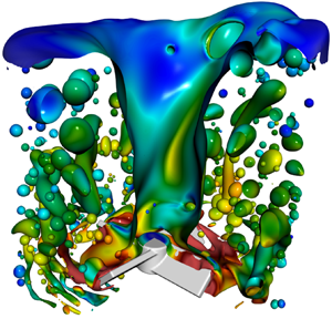
  $D/T = 0.5$. A snapshot from a typical simulation is displayed in figure 1(b), which provides an example of the level of complexity associated with the flows under consideration in the present work.

Figure 1. (a) Schematic illustration of the computational domain for the oil–water mixing system, which corresponds to a stirred vessel filled with oil and water in the upper and lower halves, respectively, with a pitched blade turbine immersed in the water phase. The domain is of size  $8.6 \times 8.6 \times 12.75$ cm
 $^3$ and it is divided into
  $4 \times 4 \times 6$ subdomains. The Cartesian structured grid per subdomain is 64
 $^3$, which gives a total grid number of
  $256 \times 256 \times 384$. (b) An illustrative snapshot of the interface at
  $t=25\times T$ coloured by velocity field for
  $f=7$ Hz; here, a quarter of the interface is hidden to provide a clear view of the impeller and the interface in its vicinity.
Under the assumptions of incompressible and immiscible viscous fluids, the mass and momentum conservation equations are solved in a Cartesian domain  $\boldsymbol {x} = (x, y, z) \in [ 0, 8.6 ] ^2 \times [ 0, 12.75 ]$ cm
 \begin{gather} \boldsymbol{\nabla} \boldsymbol{\cdot} \bar{\boldsymbol{u}} = 0, \end{gather}
 \begin{gather}\rho \left( \frac{\partial \bar{\boldsymbol{u}}}{\partial t} + \bar{\boldsymbol{u}} \boldsymbol{\cdot} \boldsymbol{\nabla} \bar{\boldsymbol{u}} \right) = {-}\boldsymbol{\nabla} \bar{p} + \boldsymbol{\nabla} \boldsymbol{\cdot} [(\mu + \rho C_{s}^{2} \varDelta^2 | \bar{S} | )( \boldsymbol{\nabla} \bar{\boldsymbol{u}} + \boldsymbol{\nabla} \bar{\boldsymbol{u}}^T )] + \rho \boldsymbol{g} + \boldsymbol{F} + \boldsymbol{F}_{fsi}, \end{gather}
 where  $\bar {\boldsymbol {u}}$ and
  $\bar {p}$ are the ensemble-averaged fluid velocity and pressure, respectively,
  $t$ denotes time and
  $\boldsymbol {g}$ is the gravitational acceleration. In (2.2), we use a single-field formulation for the density
  $\rho$ and viscosity
  $\mu$ expressed by
 \begin{gather} \rho ( \boldsymbol{x}, t ) = \rho_o + ( \rho_w - \rho_o ) \mathcal{H} ( \boldsymbol{x}, t ), \end{gather}
 \begin{gather}\mu ( \boldsymbol{x}, t ) = \mu_o + ( \mu_w - \mu_o ) \mathcal{H} ( \boldsymbol{x}, t ), \end{gather}
where the subscripts  $o$ and
  $w$ designate the oil and water phases, respectively. The indicator function
  $\mathcal {H}$, is essentially a numerical Heaviside function, zero in the oil phase and unity in the water phase. Here,
  $\mathcal {H}$ is resolved with a sharp but smooth transition across 3–4 grid cells, and is generated using a vector distance function
  $\varphi (\boldsymbol {x})$, positive for the water phase and negative for the oil phase, computed directly from the tracked interface (Reference Shin, Chergui and JuricShin, Chergui, & Juric, 2017; Reference Shin and JuricShin & Juric, 2009a). The density and viscosity of the water and oil phases are 998 kg
  ${\rm m}^{-3}$ and
  $10^{-3}~{\rm Pa\cdot s}$, and 824 kg
  ${\rm m}^{-3}$ and
  $5.4\,\times\, 10^{-3}~{\rm Pa\cdot s}$, respectively; the interfacial tension is
  $\sigma =0.035$ N m
 $^{-1}$. The oil phase corresponds to a type of silicone oil used in previous work (Reference Constante-AmoresConstante-Amores, 2021; Reference Constante-Amores, Kahouadji, Batchvarov, Shin, Chergui, Juric and MatarConstante-Amores et al., 2021b; Reference IbarraIbarra, 2017).
A range of impeller rotation frequencies,  $f= 1\unicode{x2013}10$ Hz, is studied which corresponds to
  $Re = 1802\unicode{x2013}18\ 026$ and
  $We = 2.19\unicode{x2013}219$ where the Reynolds and Weber numbers are respectively given by
 \begin{equation} Re = \frac{\rho_w f D^2}{\mu_w}, \quad We = \frac{\rho_w f^2 D^3}{\sigma}, \end{equation}
which provide a measure of the relative significance of inertial to viscous and interfacial tension forces. Here,  $D$ and
  $f D$ are the characteristic length and velocity scales, respectively. The large Reynolds numbers in the upper end of the
  $Re$ range motivate the use of a large eddy simulation approach; here, we employ a Smagorinsky turbulence model (Reference SmagorinskySmagorinsky, 1963) which is included in (2.2) wherein
  $C_s$ is the Smagorinsky–Lilly coefficient,
  $\varDelta =V^{1/3}$ where
  $V$ is the volume of a grid cell,
  $V={\rm \Delta} x{\rm \Delta} y{\rm \Delta} z$ and
  $|\bar {S}|=\sqrt {2\bar {S}_{ij}\bar {S}_{ij}}$ with
  $\bar {S}_{ij}$ being the strain rate tensor:
 \begin{equation} \bar{S}_{ij} = \frac{1}{2}\left(\frac{\partial{\bar{u}_i}}{\partial{x_j}} + \frac{\partial{\bar{u}_j}}{\partial{x_i}}\right) \end{equation}
(Reference Meyers and SagautMeyers & Sagaut, 2006; Reference PopePope, 2000, Reference Pope2004). In the current work,  $C_s=0.2$, which is an intermediate value in the range
  $0.1\unicode{x2013}0.3$ quoted in the literature (Reference DeardorffDeardorff, 1970; Reference LillyLilly, 1966, Reference Lilly1967; Reference McMillan and FerzigerMcMillan & Ferziger, 1979; Reference PopePope, 2000); setting
  $C_s = 0$ eliminates the turbulence model and (2.2) reduces to the Navier–Stokes equations. Finally, we solve the large eddy simulation filtered equations without any specific turbulence model for the interface dynamics.
The forces  $\boldsymbol {F}$ and
  $\boldsymbol {F_{fsi}}$ in (2.2) denote the local surface tension and the solid–fluid interaction forces, respectively, where
  $\boldsymbol {F}$ is defined using a hybrid formulation (Reference Shin, Chergui and JuricShin et al., 2017, Reference Shin, Chergui, Juric, Kahouadji, Matar and Craster2018)
 \begin{equation} \boldsymbol{F} = \sigma \kappa_{H} \boldsymbol{\nabla} \mathcal{H} (\boldsymbol{x},t), \end{equation}
in which  $\sigma$, the surface tension, is assumed constant. In (2.7),
  $\kappa _H$ is twice the mean interface curvature field calculated on an Eulerian grid using
 \begin{equation} \kappa_H = \frac{\boldsymbol{F}_L \boldsymbol{\cdot} \boldsymbol{G}}{\sigma \boldsymbol{G} \boldsymbol{\cdot} \boldsymbol{G}}, \end{equation}
in which  $\boldsymbol {F}_L$ and
  $\boldsymbol {G}$ are given by
 \begin{gather} \boldsymbol{F}_L = \int_{\varGamma(t)} \sigma \kappa_f \boldsymbol{n}_f \delta_f( \boldsymbol{x}- \boldsymbol{x}_f ) \, {\rm d} s, \end{gather}
 \begin{gather}\boldsymbol{G} = \int_{\varGamma(t)} \delta_f ( \boldsymbol{x}- \boldsymbol{x}_f ) \, {\rm d} s. \end{gather}
In these formulae,  $\boldsymbol {n}_f$ corresponds to the unit normal vector to the interface, and
  $ds$ is the length of the interface element;
  $\kappa _f$ is twice the mean interface curvature obtained from the Lagrangian interface. The geometric information corresponding to the unit normal
  $\boldsymbol {n}_f$ and the length of the interface element
  $ds$ in
  $\boldsymbol {G}$ are computed directly from the Lagrangian interface and then distributed on an Eulerian grid using the discrete delta function and following an immersed boundary approach (Reference PeskinPeskin, 1977). A detailed computation of the force and construction of the function field
  $\boldsymbol {G}$ can be found in Reference ShinShin (2007), Reference Shin and JuricShin and Juric (2009a, Reference Shin and Juric2009b) and Reference Shin, Chergui and JuricShin et al. (2017).
The Lagrangian interface is advected by integrating
 \begin{equation} \frac{{\rm d} \boldsymbol{x}_f}{{\rm d} t} = \boldsymbol{V}, \end{equation}
with a second-order Runge–Kutta method where the interface velocity  $\boldsymbol {V}$ is interpolated from the Eulerian velocity. Incorporating the complex geometry of the impeller and its rotation requires the implementation of the so-called direct forcing method (Reference Mohd-YusofMohd-Yusof, 1997; Reference Fadlun, Verzicco, Orlandi and Mohd-YusofFadlun, Verzicco, Orlandi, & Mohd-Yusof, 2000); this, in turn, is implemented by incorporating a fluid–solid interaction force
  $\boldsymbol {F}_{fsi}$ into (2.2) defined numerically using the latest step of the temporal integration of (2.2)
 \begin{equation} \rho \frac{\bar{\boldsymbol{u}}^{n + 1} - \bar{\boldsymbol{u}}^n}{{\rm \Delta} t} = {local}^n + \boldsymbol{F}^n_{fsi}. \end{equation}
Here, ‘local’ represents the right-hand-side terms of (2.2) that comprise the convective, pressure gradient, viscous, turbulent, gravitational and surface tension force terms; the superscripts denote the discrete temporal step in the computation.
In the solid part of the domain corresponding to the impeller, the rotational motion  $\boldsymbol {V}^{n+1}$ is enforced
 \begin{equation} \bar{\boldsymbol{u}}^{n + 1} = \boldsymbol{V}^{n + 1} = 2 {\rm \pi}f ((y-y_0 ), - ( x-x_0 )), \end{equation}
where  $(x_0, y_0) = (4.25, 4.25)$ cm are the coordinates of the impeller axis. Hence,
  $\boldsymbol {F}_{fsi}^{n}$ is given by
 \begin{equation} \boldsymbol{F}_{fsi}^n = \rho \frac{\boldsymbol{V^{n + 1}} - \boldsymbol{\bar{u}^n}}{{\rm \Delta} t} -{local}^n. \end{equation}
The no-slip condition is imposed on the velocity and the interface at the edge of the impeller parts.
The computational domain (see figure 1a) is a rectangular parallelepiped discretised by a uniform fixed three-dimensional finite-difference mesh and has a standard staggered marker-and-cell method cell arrangement (Reference Harlow and WelchHarlow & Welch, 1965). The velocity components  $\bar {u},\bar {v}$ and
  $\bar {w}$ are defined on the corresponding cell faces while the scalar variables (pressure
  $\bar {p}$ and the distance function
  $\psi$) are located at the cell centres. All spatial derivatives are approximated by second-order centred differences. The velocity field is solved by a parallel generalised minimal residual method (Reference SaadSaad, 2003) and the pressure field by a modified parallel three-dimensional Vcycle multigrid solver based on the work of Reference Kwak and LeeKwak and Lee (2004) and described in Reference Shin, Chergui and JuricShin et al. (2017). Parallelisation is achieved using an algebraic domain decomposition where communication across processes is handled by Message Passing Interface protocols.
The chosen PBT shown in figure 1(a) and described in the beginning of this section is built using a combination of primitive geometric objects (planes, cylinders and rectangular blocks) where each object is defined by a static distance function  $\psi (x,y,z)$, positive in the fluid and negative in the solid. The resulting shape in figure 1(a) corresponds to the iso-value
  $\psi (x,y,z) = 0$. Details on how to construct similar complex objects are described in Reference Kahouadji, Nowak, Kovalchuk, Chergui, Juric, Shin, Simmons, Craster and MatarKahouadji et al. (2018).
The temporal scheme is based on a second-order Gear method (Reference TuckerTucker, 2014) with implicit solution of the viscous terms of the velocity components. The time step  ${\rm \Delta} t$ is chosen at each temporal iteration in order to satisfy a criterion based on
 \begin{equation} {\rm \Delta} t = {min} \{ {\rm \Delta} t_{cap}, {\rm \Delta} t_{vis}, {\rm \Delta} t_{CFL}, {\rm \Delta} t_{int}\} \end{equation}
where  ${\rm \Delta} t_{cap}, {\rm \Delta} t_{vis}, {\rm \Delta} t_{CFL}$ and
  ${\rm \Delta} t_{int}$ represent the capillary, viscous, Courant–Friedrichs–Lewy (CFL) and interfacial CFL time steps, respectively, defined by
 \begin{gather} {\rm \Delta} t_{cap} \equiv \frac{1}{2} \left( \frac{(\rho_{o} + \rho_{w}) {\rm \Delta} x^{3}_{min}}{{\rm \pi} \sigma} \right)^{1/2}, \quad {\rm \Delta} t_{vis} \equiv {min} \left( \frac{\rho_w}{\mu_w}, \frac{\rho_o}{\mu_o} \right) \frac{{\rm \Delta} x^2_{min}}{6}, \end{gather}
 \begin{gather}{\rm \Delta} t_{CFL} \equiv {min}_{j} \left( {min}_{domain} \left( \frac{{\rm \Delta} x_j}{u_j} \right) \right), \quad {\rm \Delta} t_{int} \equiv {min}_{j} \left( {min}_{\varGamma(t)} \left( \frac{{\rm \Delta} x_j}{\| V \|} \right) \right), \end{gather}
where  ${\rm \Delta} x_{min} = {min}_{j} ({\rm \Delta} x_j)$ refers to the minimum size
  $x$ at a given cell
  $j$,
$j$,  $u_j$, and
  $V$ are the maximum fluid and interface velocities, respectively.
Mass is conserved to within  $\pm 0.02$ in all of our simulations. Our numerical procedure (Reference Shin, Chergui, Juric, Kahouadji, Matar and CrasterShin et al., 2018) has also been employed to simulate aeration in gas–liquid mixing (Reference Kahouadji, Liang, Valdes, Chergui, Juric, Shin, Craster and MatarKahouadji et al., 2022), vortex-interface dynamics and dispersion formation in turbulent water jets injected into an oil medium (Reference Constante-AmoresConstante-Amores, 2021; Reference Constante-Amores, Kahouadji, Batchvarov, Shin, Chergui, Juric and MatarConstante-Amores et al., 2021b, Reference Constante-Amores, Kahouadji, Batchvarov, Shin, Chergui, Juric and Matar2020b), the breakup of ligaments (Reference Constante-Amores, Kahouadji, Batchvarov, Seungwon, Chergui, Juric and MatarConstante-Amores et al., 2020a), the coalescence of drops with interfaces (Reference Constante-Amores, Kahouadji, Batchvarov, Seungwon, Chergui, Juric and MatarConstante-Amores et al., 2021a), the bursting of bubbles through interfaces (Reference Constante-Amores, Kahouadji, Batchvarov, Shin, Chergui, Juric and MatarConstante-Amores et al., 2021c) and the dynamics of falling films (Reference Batchvarov, Kahouadji, Magnini, Constante-Amores, Craster, Shin, Chergui, Juric and MatarBatchvarov et al., 2020). We have also carried out a validation study against the experimental work of Reference Hančil and RodHančil and Rod (1988); the results are in the Supplementary Information. To give an insight into the computational requirement, the current simulations are implemented based on the High Performance Computing service of Imperial College London, using 2 nodes of 48 CPUs for each case. All of the studied cases were computed in parallel, which took the authors two months to complete (corresponding to 25 revolutions of the impeller in this work).
3. Results and discussion
In this section, we present the spatio-temporal evolution of oil–water emulsion formation in the stirred vessel with a 4-pitch-blade turbine. First, a discussion of the vortical flow structures, and associated interfacial dynamics, is provided for the full range of  $Re$ and
  $We$ studied starting with the flows generated for the lowest rotational speeds. Then, the results of an examination of the drop size distribution evolution and its dependence on
  $Re$ and
  $We$ are presented.
3.1 Flow structures
The evolution of the flows for the two phases in the  $(x,z)$ plane at
  $y=4.25$ shows the existence of a rich dynamics, as demonstrated by the example depicted in figure 2 for the lowest Reynolds and Weber numbers studied,
  $Re=1802$ and
  $We=2.19$. A large primary vortex is created at early times (
 $t=0.5\times T$, see figure 2b), which starts at the blade tips toward the bottom of the vessel and then develops upwards near the vessel wall toward the interface. A small secondary vortex is also generated near the bottom of the impeller, which rotates radially in the opposite direction compared with the primary vortex. A suite of vortical structures accompany the development of the primary vortex which correspond to Moffatt, blade tip, Kelvin–Helmholtz and wall-end vortices (see figure 2c–e). As the velocity is continuous across the interface, and the flow in the oil phase is dragged radially inward with the meridional flow in the water phase, a large vortex is also generated in the oil phase which has the opposite circulation to that in the water. At
  $t = 6\times T$, a swirling flow is observed near the interface in the water, which centrifuges the upper oil adjacent to it radially outward generating a small vortex of opposite circulation to the large one (see figure 2f). At
  $t=9.5\times T$, a small vortex breakdown appears at the interface in the oil (see figure 2g) which grows, squeezing the large meridional flow to the fixed sidewall until it gives way to two large circulation cells with a direction of radially outward (figure 2h–k); we will discuss vortex breakdown at higher
  $Re$ and
  $We$ below. The oil flow then remains in a configuration where the original meridional flow is confined to a thin layer in the vicinity of interface while the counter one above dominates in the oil phase (see figure 2l). On the other hand, flow separation (figure 2g) occurs in the water close to the edge of the rotating impeller (as described in the work of Reference Piva and MeiburgPiva & Meiburg, 2005). The water flow is characterised by a high level of turbulence involving the development of a multitude of vortices of varying scales. Similar behaviour in the water phase was demonstrated by Reference Kahouadji, Liang, Valdes, Chergui, Juric, Shin, Craster and MatarKahouadji et al. (2022) who carried out simulations of air–water mixing in stirred vessels.

Figure 2. Spatio-temporal evolution of the vortical structures for  $Re = 1802$ and
  $We=2.19$ from an initial static state (a) until
  $t=20\times T$ (l). In this and subsequent figures, the results are displayed in the
  $(x,z)$ plane at
  $y=4.25$, and cyan and yellow are used to designate the water and oil phases, respectively, while the red solid line represents the interface location. Enlarged snapshots of the vortical structures with corresponding annotations are shown for
  $t=6\times T$ and
  $t=9.5\times T$ in
  $(m)$ and
  $(n)$, respectively.
We now present the spatio-temporal evolution of the interface shape for  $Re =7210$ and
  $We=35$ in figure 3. As the impeller rotates, the azimuthal velocity generated by the impeller exerts a torque on the interface deforming it and subsequently drags the oil in the centre downwards (see figure 3a,b). The impeller rotation is not sufficiently rapid so as to cause the interface to reach the impeller; instead, the interface deforms into a helical shape, as shown in figure 3(c). Afterwards, a long ligament detaches from the deforming interface, which subsequently breaks into a large drop and several smaller ones (figure 3d,e). When
  $t$ >
$t$ > $14\times T$, the dispersed large drop retracts to the deforming interface, spirally stretching in the meantime to become longer and thinner before attaching to the impeller (see figure 3f–i). The ligament detachment, breakup and retraction cycle is repeated until the system reaches a dynamic steady state where small drops remain dispersed in the water phase together with the deforming interface in the shape of a Newton's Bucket (see figure 3j–l). The existence of both ligament retraction, due to the action of interfacial tension, and elongation, due to the interaction with the turbulent flow in the water phase, highlights the presence of the delicate interplay amongst the various competing forces which results in the complexity associated with the mixing process.

Figure 3. Spatio-temporal evolution of interface for  $Re=7210$ and
  $We=35$ from a state where the interface starts to deform (a) until
  $t=20\times T$ (l).
An enlarged view of the breakup process is provided in figure 4, which presents the concurrence of multiple drop pinch-offs along one single ligament. Close inspection reveals that the ligament initially takes time to elongate and thin giving rise to thread-like regions between nodules, which continue to thin until they break up into individual droplets via a Rayleigh–Plateau mechanism. To explain the phenomenon observed within our mixing system, we examine closely the vorticity profiles around the ligament. Figure 5 presents four horizontal planes that depict the flow, coloured according to the magnitude of the vorticity. As shown in these plots, which also illustrate the position of the ligament relative to the vorticity distribution in the flow, the ligament lies in the high vorticity region generated by the impeller rotation. The interaction of the vorticity with the interface contributes to the instability of the ligament and this is particularly pronounced in the near-impeller regions in which the magnitude of the vorticity is significantly larger than those close to the vessel walls.

Figure 4. Enlarged views of ligament breakup for  $Re = 9013$ and
  $We=55$ at
  $16.375 T$ and
  $16.625T$.

Figure 5. Vorticity in the ligament surroundings for  $Re = 9013$ and
  $We=55$. Four horizontal planes generated for
  $z=0.82,0.70,0.65,0.58$, corresponding to the red-, blue-, green- and yellow-labelled planes, are coloured according to the vorticity magnitude. The side and top views of the ligament shown in the middle and parts of the ligament are highlighted by white solid lines in the vorticity panels.
Next, we return to the occurrence of vortex breakdown in the oil phase which we had discussed above and note that it is also observed in the range of  $Re=1802\unicode{x2013}9013$ and
  $We=2.19\unicode{x2013}55$ where the interface remains in a dynamic steady state assuming a Newton's Bucket-like shape, as shown in figure 6. The top panels of figure 6 highlight the vortical structures when the flow has reached a dynamic steady state where the vortex breakdown has developed into the dominant circulation cells along with the counter-rotating ones confined to a thin layer near the interface. For the higher
  $Re$ and
  $We$ cases shown in figure 6(a–e), the vortex breakdown appears earlier, for example, at around
  $t=7\times T$ for
  $(Re,We) = (9013,55)$ compared with
  $t=9.5\times T$ for
  $(Re, We) = (1802,2.19)$ as shown in figure 2.

Figure 6. Vortical flow structures, top panels, and their corresponding interfacial shape, bottom panels, for  $(Re,We)$ combinations of (1802,2.19), (3605,8.76), (5408,19), (7210,35) and (9013,55) shown in (a–e), respectively, at
  $t=25\times T$ when the flow has reached a dynamic steady state.
The bottom panels of figure 6 also show that, with increased  $Re$ and
  $We$, the depth of Newton's Bucket increases, approaching the impeller with the interface assuming a teardrop shape. It may be possible to use the onset of vortex breakdown as an indicator of, and a surrogate for, the fact that the interface will remain sufficiently far from the impeller, and therefore unattached to it, at steady state. A methodology that focuses on the detection of vortex breakdown (if it occurs) for a given set of parameters, and then tracks the dependence of the breakdown over a range of such parameters, can lead to a map in
  $(Re,We)$ space in which the region of limited mixing is demarcated; such an approach would obviate the need for lengthy computations to resolve the intricate and rapidly evolving interfacial dynamics.
We now consider a range of  $Re$ and
  $We$ for which no retraction of the deforming interface from the impeller is observed. In figure 7, we show the spatio-temporal evolution of the vortical structures for
  $Re=12\ 618$ and
  $We=107$ from an early-time state (at
  $t=2\times T$, see figure 7a) to a stage of the flow at which the deforming interface has reached the impeller (at
  $t=9\times T$, see figure 7f). During the early stages of the flow, the vortical structures observed are similar to those depicted in figure 2 discussed above. Instead of the appearance of vortex breakdown seen at lower
  $Re$ and
  $We$, the streamline configuration at higher
  $Re$ and
  $We$ indicates a strong tendency of the interface to be deflected towards the impeller (see figure 7e). Although the water phase is dominated by the primary vortex, there are a number of secondary vortices close to the vessel sidewall in the vicinity of the interface which act to pump the water upward along the wall (see figure 7c–f). In figure 8, we illustrate the spatio-temporal evolution of interface shape for
  $(Re,We)=(10~816,78)$ and (12 618,107) shown for
  $t=8 -25\times T$. After the interface reaches the impeller (see figure 8b), it is further stretched radially and long oil ligaments are created when the impeller blades cut through the rotating curtains (see figure 8c). Long ligaments subsequently stretch to become thinner until pinch-off occurs, giving rise to multitudes of smaller drops (see figure 8d). Then, the deforming interface evolves differently depending on the value of
  $Re$ and
  $We$. Whereas for
  $Re=9013$ and
  $We=55$ the interface eventually detaches from the impeller and no further ligaments are generated, as shown in figure 4, the formation of new ligaments remains in place at the higher
  $Re$ and
  $We$ (see figure 8e). The small drops created from ligament breakup either travel upwards under the action of buoyancy, eventually merging with the oil phase, or remain dispersed in water until they coalesce with other drops. As a result, although the number of dispersed drops decreases with time for
  $Re=9013$ and
  $We=55$, this is not the case at higher
  $Re$ and
  $We$ as the drops ‘lost’ due to coalescence with the oil–water interface are replenished via continual ligament formation and subsequent breakup (see figure 8f). A discussion of the evolution of the dispersed drop number and size distribution will be provided in § 3.2.

Figure 7. Spatio-temporal evolution of the vortical structures for  $Re=12\ 618$ and
  $We=107$ at
  $t=2-9\times T$ shown in (a–f), respectively.

Figure 8. Spatio-temporal evolution of the interface toward the development of an oil-in-water emulsion for  $(Re,We)=(10\ 816,78)$ and (12 618,107) shown in the top and bottom panels, respectively, for
  $t=8\times T$ between
  $25\times T$ in (a–f), respectively.
At larger  $Re$ and
  $We$, the vortical structures in the oil and water phases during the early and intermediate stages of the dynamics resemble those discussed above; this is exemplified by figures 9(a)–9(f) in which we show the evolution of these structures for
  $Re=18\ 026$ and
  $We=219$ between
  $t=2\times T$ and
  $9\times T$ which culminates in the interface reaching the impeller. Inspection of figure 9(g–l), however, in which we illustrate the evolving interfacial dynamics, reveals that drop coalescence dominates over breakup. In contrast to the lower
  $Re$ and
  $We$ cases discussed above, a larger torque is generated in the present case which results in a deforming interface of a helical shape with four rotating curtains (see figure 9g). Following their formation, the long ligaments merge to form a relatively large mass of oil that collects around the bottom of the vessel before breaking up into smaller drops as they are rapidly and continually created from the impeller tips (see figure 9h). As can be seen in figure 9(i), the dispersed phase in this high
  $Re$ case is composed mainly of stretched oil ligaments rather than the individual drops observed to accompany the flow at lower
  $Re$. With increasing time, an increasing amount of oil is entrained into the water phase; as a result, the latter is displaced upwards along the vessel sidewalls lifting the interface as can be seen in figure 9(j,k). At
  $t=25\times T$, the dynamics is characterised by complex interfacial topology. It is notable that the number of small droplets has decreased due to coalescence giving way to large dispersed-phase structures resulting from the merging of ligaments and drops, as shown in figure 9(l). The drop size distribution as a function of the impeller speed is discussed next.

Figure 9. Spatio-temporal evolution of the vortical structure between  $t=2\times T$ and
  $9\times T$, (a–f), and of the interface between
  $t=9\times T$ and
  $25\times T$, (g–l), for
  $Re=18\ 026$ and
  $We=219$.
3.2 Drop size distribution
From an industrial point of view, it is often important to track the evolution of the dispersed-phase statistics and metrics in terms of number of drops, their size distribution, the interfacial area and hold up. Figure 10 presents the temporal evolution of the number of dispersed drops ( $t=5\unicode{x2013}25\times T$) for
  $f = 5\unicode{x2013}10$ Hz (
 $Re=9013\unicode{x2013}18\ 026$ and
  $We=55\unicode{x2013}219$), along with the corresponding interface shapes at
  $t= 25\times T$. For all displayed frequencies, no dispersed drop appears until there is a steep increase from zero drop count at
  $t\approx 8\times T$, caused by the above-mentioned Rayleigh–Plateau-type breakup from long ligaments. In addition, the appearance of the dispersed drops occurs earlier with increasing impeller speed due to the accelerated deviation of the interface and its earlier interaction with the impeller to produce ligaments. Furthermore, figures 8(c) and 9(h) provide clear evidence that, when the rotation frequency is increased, a larger part of the deforming interface contacts the impeller and therefore more ligaments are produced at the beginning, which corresponds to the steeper increase, as shown in figure 10. After that, the number of dispersed oil drops for
  $f=5$ Hz falls off gently since the deforming interface no longer makes contact with the impeller while dispersed drops tend to coalesce with the oil overlying the water phase. With increasing frequency, the dispersed oil drop number continues to increase until the breakup rate balances that of coalescence. For cases with
  $f \geq 8$ Hz, an over-shooting peak is observed before the number decreases towards a dynamic steady state. We posit that this phenomenon is due to the fact that the larger amount of ligaments and drops produced simultaneously increases the coalescence probability in the system. As a result, there exists a stage where the coalescence rate is larger than the breakup rate, giving rise to the reduction in drop counts.

Figure 10. Temporal evolution of the number of dispersed drops for frequencies  $f=5,6,7,8,9,10$ Hz, which correspond to
  $Re=9013\unicode{x2013}18 026$ and
  $We=55\unicode{x2013}219$. Snapshots of the interface shapes at
  $t=25\times T$ are also presented for each frequency. The black arrow indicates the earlier drop occurrence and the steeper increase from zero drop count when impeller speed is increased.
It is evident from figure 10 that the steady number of dispersed drops has a non-monotonic dependence on the impeller speed while its over-shooting peak increases with increasing rotation frequencies. On the other hand, our results also indicate that the interfacial area of the dispersed phase at steady state ( $t=25\times T$) shows no such dependence as shown in figure 11(a). This interfacial area is calculated as
  $A_{d}/A_{cap}$, where
  $A_d$ refers to the surface area of all dispersed drops and
  $A_{cap}$ is the sphere surface area with the capillary length as its diameter. The interfacial area appears to be proportional to the increased impeller speed (up to
  $f=10$ Hz) even though the number of dispersed drops reaches its peak at an intermediate frequency (
 $f=7$ Hz). The reason for this is that at larger frequencies, long ligaments, with larger interfacial area, dominate the dispersed-phase morphology (see figure 9). From figure 11(a), the optimal impeller speed can be selected depending on the relative importance of the interfacial area and dispersed drop number to the particular application in question.

Figure 11. (a) Number of drops (blue line, inverted triangle markers) and interfacial area (red line, cross-shaped markers) of the dispersed oil phase. (b) Box plot distribution of the drop size (outliers are not shown here), at  $t=25\times T$ for frequencies
  $f=5,6,7,8,9,10$ Hz, which correspond to
  $Re=9013\unicode{x2013}18\ 026$ and
  $We=55\unicode{x2013}219$. Here, the median value of
  $V_d/V_{cap}$ is indicated by the horizontal red lines.
For all frequencies, we examine the drop size distribution at  $t=25\times T$ for
  $f=5\unicode{x2013}10$ Hz (
 $Re=9013\unicode{x2013}18\ 026$ and
  $We = 55\unicode{x2013}219$). We define a dimensionless ‘drop’ size as
  $V_d/V_{cap}$, where
  $V_d$ refers to the volume of a dispersed phase entity (which can be a deformed drop or a ligament) and
  $V_{cap}$ is a spherical drop whose diameter corresponds to the capillary length scale,
  $\sqrt {\sigma /{\rm \Delta} \rho g}$; here,
  ${\rm \Delta} \rho$ is the difference in density between the oil and water phases. A box plot distribution of
  $V_d/V_{cap}$ at
  $t=25\times T$ is shown in figure 11(b) indicating that the overall trend is that an increase in frequency leads to a narrower distribution and smaller median drop size, which is consistent with the conclusion of previous studies (Reference Pacek, Man and NienowPacek et al., 1998; Reference Zhou and KrestaZhou & Kresta, 1998b). This trend is also demonstrated in figure 12 where the fitted drop size distribution is plotted against logarithmic
  $V_d/V_{cap}$. For
  $f=5$ Hz, the drop size is best fitted to a normal distribution, while for higher impeller speeds, the drop size follows a generalised logistic distribution. The narrow distribution for
  $f=5$ Hz indicates that relatively large (median value to the left figure 12) drops of well-distributed size are produced; on the other hand, with increasing impeller speed, the median drop size moves to smaller sizes, while a skewed shape towards the more frequently produced small drops is observed. Additionally, a drop size map for
  $f=7$ Hz is also shown in figure 12 where all the dispersed-phase entities are classified into three size categories and coloured accordingly. This gives a clear indication that the ‘large-sized’ drops contain the long ligaments that have not broken up entirely, whereas the ‘small-’ and ‘moderate-sized’ drops are composed of individual droplets of various sizes.

Figure 12. Drop size distribution of the dispersed oil phase at  $t=25\times T$ for
  $f=5,6,7,8,9,10$ Hz (
 $Re=9013\unicode{x2013}18\ 026$ and
  $We=55\unicode{x2013}219$). The attached image shows a drop size map for
  $f=7$ Hz at
  $t=25\times T$ where all the dispersed phases are coloured by red, yellow and blue according to their size as small, moderate and large, respectively.
4. Conclusion and perspective
In this paper, using our high-fidelity three-dimensional simulations, we study the effect of impeller rotational speed on the complex interfacial dynamics during oil–water mixing in a stirred vessel with a 4-pitch-blade turbine; we explore rotational speeds in the range  $f=1\unicode{x2013}10$ Hz, which correspond to Reynolds and Weber number ranges of
  $Re = 1802\unicode{x2013}18\ 026$ and
  $We=2.19\unicode{x2013}219$, respectively. We have shown that the interface shape and vortical structures within such a system are strongly dependent on the impeller speed. In particular, we have demonstrated the possibility of using vortex breakdown as an indicator that the interface undergoes little breakup due to very little interaction with the impeller. In addition, we have also presented a drop size analysis over the full range of frequencies studied in terms of temporal evolution of the dispersed drop number and its size distribution at steady state, and shown that an optimal impeller speed can be selected depending on the needs of the application in question. In future research, it can be interesting to explore other effects on the mixing system, which include impeller geometry, fluid phase rheology and the presence of surfactants; the latter are of particular interest since surfactants may be present in the system either as a contaminant or by design.
Funding
This work is supported by the Engineering  $\&$ Physical Sciences Research Council, UK, through the MEMPHIS (EP/K003976/1) and PREMIERE (EP/T000414/1) Programme Grants, and by computing time at HPC facilities provided by the Research Computing Service of Imperial College London. D.J. and J.C. acknowledge support through HPC/AI computing time at the Institut du Developpement et des Ressources en Informatique Scientifique (IDRIS) of the Centre National de la Recherche Scientifique (CNRS), coordinated by GENCI (Grand Equipement National de Calcul Intensif) Grant 2022 A0122B06721. O.K.M. also acknowledges funding from PETRONAS and the Royal Academy of Engineering for a Research Chair in Multiphase Fluid Dynamics, and the PETRONAS Centre for Engineering of Multiphase Systems. Simulations have been performed using code BLUE (Reference Shin, Chergui and JuricShin et al., 2017) and the visualisations have been generated using Paraview.
Declaration of interest
The authors report no conflict of interest.
Author contributions
O.K.M. secured the funding; F.L., L.K., J.P.V., D.J. and O.K.M. contributed to the design of the research plan and manuscript editing; F.L., L.K., S.S., J.C. and D.J. contributed to the computations.
Data availability statement
Raw data are available from the corresponding author L.K.
Ethical standards
The research meets all ethical guidelines, including adherence to the legal requirements of the study country.


 Open access