


Introduction
Gas extraction from the large onshore field in the Groningen region, the Netherlands, has caused induced seismicity with a maximum magnitude of ML = 3.6 to date (van Geuns & van Thienen-Visser, Reference van Geuns and van Thienen-Visser2017; Muntendam-Bos et al., Reference Muntendam-Bos, Roest and De Waal2017). During recent years, a Ground Motion Model (GMM) has been developed (Bommer et al. Reference Bommer, Dost, Edwards, Kruiver, Ntinalexis, Rodriguez-Marek, Stafford and van Elk2017a, b) to facilitate the seismic hazard and risk assessment (Van Elk et al., Reference van Elk, Bourne, Oates, Bommer, Pinho and Crowley2019). Many assumptions were made during the early development of the GMM. For example, the very first Ground Motion Prediction Equation for Groningen included only linear site effects for field-wide average conditions (Bommer et al., Reference Bommer, Dost, Edwards, Stafford, van Elk, Doornhof and Ntinalexis2016). As more data became available, the model was refined stepwise and new types of validations could be performed. The model was further refined through the addition of geological information representing the heterogeneity of the sediments in the region and soil properties such as shear-wave velocity (V S) (Kruiver et al., Reference Kruiver, van Dedem, Romijn, de Lange, Korff, Stafleu, Gunnink, Rodriguez-Marek, Bommer, van Elk and Doornhof2017a, b), conversion of local magnitude to moment magnitude (Dost et al., Reference Dost, Edwards and Bommer2018, Reference Dost, Edwards and Bommer2019), addition of magnitude and distance dependence for amplification (Stafford et al., Reference Stafford, Rodriguez-Marek, Edwards, Kruiver and Bommer2017), better predictions of motions at the reference rock horizon (Edwards et al., Reference Edwards, Zurek, van Dedem, Stafford, Oates, van Elk, de Martin and Bommer2019) and refinement of component-to-component variability and spatial correlation (Stafford et al., Reference Stafford, Zurek, Ntinalexis and Bommer2019).
The GMM is a regional model, spanning a region of ∼40 km by 45 km. For a complete assessment of seismic hazard and risk, it is important that epistemic uncertainty and aleatory variability of the entire model chain is captured using a probabilistic approach. The GMM consists of a part predicting motions at the reference baserock horizon at ∼800 m depth and a part describing the site response between this level and the surface. For the GMM, the large field has been discretised into zones. Within each zone, amplification functions are defined consisting of median amplification factors (AF) as a function of magnitude M , rupture distance R rup and spectral acceleration at the reference baserock horizon. In these amplification functions, aleatory variability is represented by site-to-site variability ϕ S2S (Rodriguez-Marek et al., Reference Rodriguez-Marek, Kruiver, Meijers, Bommer, Dost, van Elk and Doornhof2017) in the uncertainty model. The apparent aleatory variability in the amplification functions for each zone needs to reflect an element of the spatial variability of AFs over these zones. The V S is, among others, an important parameter in site response calculations. Other parameters include the site fundamental period obtained from earthquake horizontal-to-vertical spectral ratios (e.g. Zhu et al., Reference Zhu, Pilz and Cotton2020 and van Ginkel et al., Reference van Ginkel, Ruigrok, Stafleu and Herber2022). In the GMM, V S profiles were used in the site response calculations. Therefore, we concentrate on this parameter in this study. Information about V S can be obtained from measurements, such as seismic cone penetration tests (SCPT), downhole and cross-hole tomography or Multispectral Analysis of Surface Waves. The invasive methods (SCPT, shallow boreholes) typically reach to a depth of several tens of metres. Deeper information can be obtained from well logs from the oil and gas industry (nlog.nl) and from processing of seismic reservoir imaging surveys. For the Groningen region, the V S model consists of a combination of local measurements of V S , reprocessing of groundroll of legacy regional seismic survey data, the prestack depth migration velocity model used for imaging of the reservoir (Kruiver et al., Reference Kruiver, van Dedem, Romijn, de Lange, Korff, Stafleu, Gunnink, Rodriguez-Marek, Bommer, van Elk and Doornhof2017a) and geological models (Kruiver et al., Reference Kruiver, Wiersma, Kloosterman, De Lange, Korff, Stafleu, Busschers, Harting and Gunnink2017b). During recent years, new V S data in Groningen have become available. Passive seismic surveys on various large 40–60 km2 and ∼1 km2 small square arrays of flexible seismic monitoring networks were conducted in Groningen targeted at gathering V S information to a depth of 800 m and 100 m, respectively. These data provide an independent source of V S , although of limited spatial extent. These square arrays of so-called field V S data provide an opportunity to check whether the level of spatial variability in the GMM using model V S data is sufficient. Comparing site response amplification using either model V S or field V S for two selected blocks of flexible array data provides insights on the sensitivity of the results to variations in V S .
The general workflow (Fig. 1) is reflected in the structure of the paper. This paper first presents the V S datasets from field measurements from surface to 800 m depth and more detailed datasets from surface to 100 m depth. The V S dataset from the field to 800 m depth (Chmiel et al., Reference Chmiel, Mordret, Boué, Brenguier, Lecocq, Courbis, Hollis, Campman, Romijn and van der Veen2019) lacked detail in the top ∼100 m (by design). The resolution in the top 100 m was improved with new field data. The acquisition and processing of the new V S data to 100 m depth are included in the paper. The next section describes the site response methodology, including the input datasets. Next, the comparison of amplification results between model V S and field V S shows that model AF and field AF are comparable or that the model AF is conservative. In the discussion, the spatial variation from the GMM is compared to the recordings of an earthquake that was recorded by one of the flexible array network blocks.
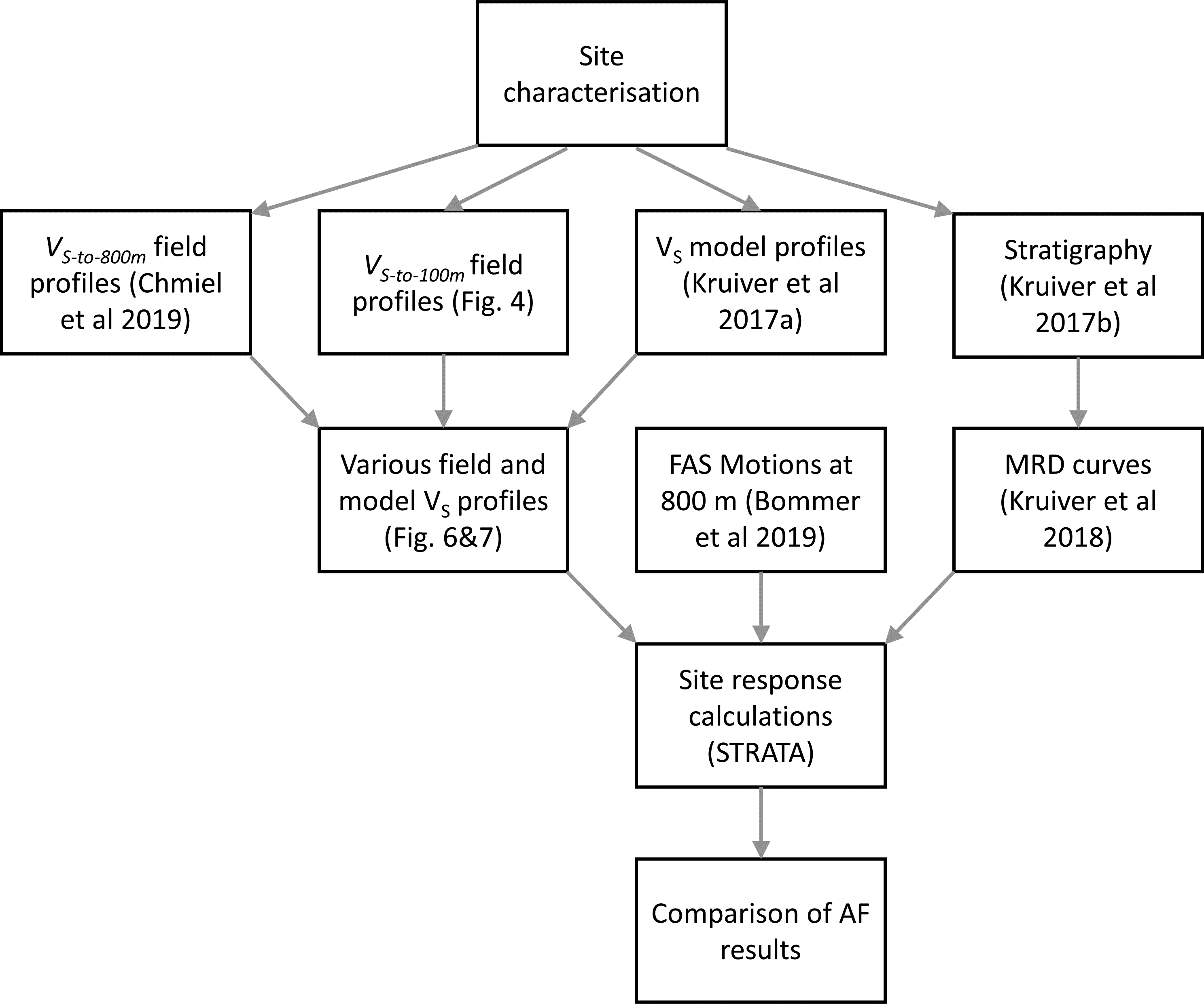
Fig. 1. Flow chart of site characterisation, VS profile construction, the other inputs for site response calculations – Fourier Amplitude Spectra (FAS) and Modulus Reduction and Damping (MRD) curves – and interpretation of the results.
New local field VS data from flexible array measurements
The new local V S data from field measurements consist of two depth ranges. During the first phase of deployment of the flexible array networks, the target depth for V S was 800 m (referred to as V S-to-800 m), corresponding to the average depth of the base of the North Sea Supergroup. The North Sea Supergroup consists of unconsolidated sediments. Especially the top tens of metres contain very soft Holocene sediments of peat, clay and sand with low V S . The Holocene deposits form a wedge with maximum thickness of ∼20 m in the northern part of Groningen to 0 m in the southern part of Groningen where Pleistocene sands are present at the surface. More elaborate descriptions about the regional geology and local stratigraphy are given in Kruiver et al. (Reference Kruiver, Wiersma, Kloosterman, De Lange, Korff, Stafleu, Busschers, Harting and Gunnink2017b). The deeper part of the Groningen V S model (Kruiver et al., Reference Kruiver, van Dedem, Romijn, de Lange, Korff, Stafleu, Gunnink, Rodriguez-Marek, Bommer, van Elk and Doornhof2017a) is based on the pre-stack depth migration model of the seismic data used for imaging of the reservoir. The depth migration model is laterally smooth. The time-to-depth conversion is based on compressional wave velocities (V P ). These V P data were then converted to a V S model based on data from only two wells in Groningen, using a varying Poisson’s ratio for the Upper North Sea Group (generally between 0.45 and 0.47) and a constant Poisson’s ratio of 0.446 for the Lower North Sea Group (Kruiver et al., Reference Kruiver, van Dedem, Romijn, de Lange, Korff, Stafleu, Gunnink, Rodriguez-Marek, Bommer, van Elk and Doornhof2017a). Because of this limited constraint, there was a desire to calibrate this part of the V S model with independent V S measurements. The results in Chmiel et al. (Reference Chmiel, Mordret, Boué, Brenguier, Lecocq, Courbis, Hollis, Campman, Romijn and van der Veen2019) showed good agreement between the Kruiver et al. (Reference Kruiver, van Dedem, Romijn, de Lange, Korff, Stafleu, Gunnink, Rodriguez-Marek, Bommer, van Elk and Doornhof2017a) model and the models derived from the ambient noise data, except for in the shallow part, which has a great impact on ground motion.
Preliminary site response calculations showed that the vertical resolution of the resulting V S profiles was insufficient in the top ∼60 m. This can be attributed to the relatively large spacing of the stations (350 m) necessary to reach the target depth of 800 m. Therefore, during the second phase of flexible array network deployment, several smaller arrays were installed to collect data for a target depth of 100 m (referred to as V S-to-100 m). The processing and results for example blocks with target depth of 800 m is published in Chmiel et al. (Reference Chmiel, Mordret, Boué, Brenguier, Lecocq, Courbis, Hollis, Campman, Romijn and van der Veen2019). Two blocks of new V S profiles were selected for this study, located at Borgsweer and Loppersum (Fig. 2). The acquisition, processing and resulting field V S data are described in this section.

Fig. 2. Left: Outline of Groningen gas field in the Netherlands, including a 5 km buffer. Right: Location of flexible array networks. The background image shows the depth of the transition from Holocene to Pleistocene sediments (red shades to a depth of 30 m, dark green shades to 16 m, light green and cyan shades to 4 m, Pleistocene at surface for yellow shades) (Vos et al., Reference Vos, Bazelmans, Weerts and van der Meulen2011). Coordinates are in metres in the Dutch RD system.
A total of approximately 440 GSX-3 24bit nodal recording devices (nodes) with 3-component sensors from Geospace (GF-One LF 5 Hz) were deployed in a square or rectangular grid. The initial design was based on Nyquist sampling criteria as well as requirements to prevent cycle-skipping during velocity inversion. The sensitivity of Rayleigh waves to V S depends on frequency and the velocity structure. Figure 3 shows that frequencies as low as 0.3 Hz are required to achieve significant sensitivity to V S at a depth of 800 m based on the Groningen model V S profiles (Kruiver et al., Reference Kruiver, van Dedem, Romijn, de Lange, Korff, Stafleu, Gunnink, Rodriguez-Marek, Bommer, van Elk and Doornhof2017a). Power spectral density of passive data recorded by the nodes indicates that instrument noise dominates below 0.1 Hz and that frequencies higher than 0.3 Hz are well recorded (Chmiel et al., Reference Chmiel, Mordret, Boué, Brenguier, Lecocq, Courbis, Hollis, Campman, Romijn and van der Veen2019).

Fig. 3. Fundamental mode and first overtone Rayleigh wave sensitivity kernels at 0.3 Hz (left) and 0.8 Hz (right) for the Groningen VS structure (Kruiver et al., Reference Kruiver, van Dedem, Romijn, de Lange, Korff, Stafleu, Gunnink, Rodriguez-Marek, Bommer, van Elk and Doornhof2017a).
The nominal node spacing was based on estimates of minimum expected wavelengths. The extent of the array was based on sampling a minimum number of cycles of the maximum expected wavelengths to avoid near-source effects. For the target depth of 800 m, the nominal node spacing was 350 m for an array size of 6–10 km. The design of the V S-to-100 m array is a scaled version of the V S-to-800 m array. For the target depth of 100 m, the array blocks measured 1 km × 1 km and the nominal node spacing was 50 m.
Each flexible array was deployed for approximately 30 days, measuring ambient noise with a sample frequency of 250 Hz. The large array with a target depth of 800 m spanned 6.5 km by 10 km for Borgsweer (December 2016/January 2017) and 8 km by 8 km for Loppersum (October/November 2016). The small array with a target depth of 100 m measured 1 km × 1 km in both cases. Data were collected in April/May 2018 for Borgsweer and in December 2017/January 2018 for Loppersum.
The ambient noise surface wave tomography uses ambient seismic noise from natural and anthropogenic sources for subsurface imaging and monitoring. Cross-correlation between receiver pairs is used to extract an estimate of the Green’s function (e.g. Bensen et al., Reference Bensen, Ritzwoller, Barmin, Levshin, Lin, Moschetti, Shapiro and Yang2007; Lecocq et al., Reference Lecocq, Caudron and Brenguier2014) and analysis of dispersion of surface wave from the cross-correlated data generates a near-surface velocity model (Shapiro and Campillo, Reference Shapiro and Campillo2004; Mordret et al., Reference Mordret, Landès, Shapiro, Singh, Roux and Barkved2013; Boué et al., Reference Boué, Denolle, Hirata, Nakagawa and Beroza2016).
The 100 m target depth dataset was processed using the same approach as the 800 m target depth dataset (Chmiel et al., Reference Chmiel, Mordret, Boué, Brenguier, Lecocq, Courbis, Hollis, Campman, Romijn and van der Veen2019). In the following, we summarise the processing workflow using the Borgsweer flexible array dataset. The Loppersum array was processed in the same way. First, we performed a quality check of the recorded signals for every station through the probabilistic power spectral density. Next, following the procedure in Bensen et al. (Reference Bensen, Ritzwoller, Barmin, Levshin, Lin, Moschetti, Shapiro and Yang2007) and Chmiel et al. (Reference Chmiel, Mordret, Boué, Brenguier, Lecocq, Courbis, Hollis, Campman, Romijn and van der Veen2019) the records were correlated for the 97,020 possible station pairs to retrieve the surface waves (Fig. 4, step a). Beamforming analysis (Rost & Thomas, Reference Rost and Thomas2002; Boué et al., Reference Boué, Roux, Campillo and de Cacqueray2013) shows that the ambient noise direction agrees well with the general direction of the North Sea (Figure S1 in Supplementary Material). This is also supported by azimuthal distribution of dispersion curves used in surface wave tomography (Figure S2 in Supplementary Material).

Fig. 4. Flow chart of the processing workflow used for computing the VS profiles from ambient seismic noise. Steps are identical for V S-to-800 m and V S-to-100 m . The illustrations show examples from V S-to-100 m from Borgsweer. Numbers on the axes are not shown for better readability. The panels serve to illustrate the method, rather than the results.
The group velocity dispersion curves were picked automatically (Fig. 4, step b) using the frequency-time analysis algorithm (Dziewonski et al., Reference Dziewonski, Bloch and Landisman1969). All the dispersion curves for station pairs separated by less than 200 m were rejected to ensure reliable dispersion measurements, which requires the minimal interstation spacing of at least three wavelengths (Bensen et al., Reference Bensen, Ritzwoller, Barmin, Levshin, Lin, Moschetti, Shapiro and Yang2007). Finally, after computing the statistics of all remaining dispersion curves, outliers were rejected defined as dispersion curves for which at least one point falls outside the boundary of ± 70 m/s from the most probable group velocity dispersion curve. This confidence interval was chosen empirically based on the probability density functions of the Rayleigh and Love wave fundamental mode group velocity as 20-35% of the most probable group velocity. The average phase velocity dispersion curves were calculated using a frequency-wavenumber analysis on stacked cross-correlations (see Chmiel et al., Reference Chmiel, Mordret, Boué, Brenguier, Lecocq, Courbis, Hollis, Campman, Romijn and van der Veen2019 for details).
The dispersion curves were inverted in the period band [0.3–1.5] s (Fig. 4, step c) with a regular step of 0.1 s and regionalised into a regular grid of 135 m by 90 m cells (in North and East directions) using the approach of Mordret et al. (Reference Mordret, Landès, Shapiro, Singh, Roux and Barkved2013) for both Love and Rayleigh wave tomography. This first inversion leads to series of group velocity maps that describe local dispersion curves (i.e. group velocity vs. frequency) at each single cell of the map (Fig. 4, step d).
Finally, the Rayleigh and Love local group dispersion curves and Rayleigh and Love average phase velocity dispersion curves at depth were jointly inverted to obtain local 1D V S depth profiles for each cell (Fig. 4, step e). A Monte-Carlo approach based on a Neighbourhood Algorithm (Sambridge, Reference Sambridge1999; Mordret et al., Reference Mordret, Landès, Shapiro, Singh and Roux2014) was used to invert the dispersion curves at depth. Initial 1D models were defined for each point of the regionalised grid using a priori knowledge on the depth of the Holocene layer (first layer) and 30 homogeneous layers with constant thickness below this depth. The general 1D velocity profile is parameterised by a linear combination of five cubic splines modified by a power-law profile backbone. In total, we invert for eight parameters: two parameters describing a power-law increase of velocity with depth after the first layer to account for the compaction of the sediments, five parameters as weights for cubic splines super-imposed on the power-law profile to account for velocity anomalies departing from the power-law and one parameter defining the velocity in the half-space below 120 m depth. Our parametrisation allows for the velocity inversions. A total of 16,000 models were sampled. During the inversion, the P-wave velocity is scaled to V S using a V P /V S ratio of 4.2 (Kruiver et al., Reference Kruiver, van Dedem, Romijn, de Lange, Korff, Stafleu, Gunnink, Rodriguez-Marek, Bommer, van Elk and Doornhof2017a), and the density is scaled to V P using the empirical relationship of Brocher (Reference Brocher2005). The final 1D model for each cell is the average of the 300 best models with the lowest misfits. The number of 300 best models was chosen following previous studies in the area (Chmiel et al., Reference Chmiel, Mordret, Boué, Brenguier, Lecocq, Courbis, Hollis, Campman, Romijn and van der Veen2019). Uncertainty for our VS model is defined as the standard deviation of the distribution of the 300 best velocity models at each depth. To obtain the final velocity cube, we interpolate the 30-layer 1D models every 2 m at depth. The ensemble of the final 1D models computed for each cell constitutes the final 3D V S model.
Figure 5 shows two examples of local depth inversion along with the final misfit map of the inversion results for Borgsweer area. The normalised misfit map (Fig. 5b) indicated a good match between the dispersion measurements and the model, with misfit lower than 0.3 over most of studied area. Higher misfits are encountered in the western part of the area. Figure 5c–d shows examples of inversion results in this zone. The parameters explored by the model poorly fit the group velocity for Love waves at periods of 0.95s to 1.45s. Figure 5c shows an example of good misfits that are achieved for most points of the depth inversion. Even though the fit is better than Fig. 5b, the parameters explored by the model poorly fit the group velocity for Love waves at periods of 1.25–1.45 s. In general, we observe that the area of high misfits corresponds to the high velocity zone. In a geologically complex area, the depth inversion can give more uncertain results. For example, this discrepancy can be explained by the presence of anisotropy, or else of noisier Love waves data (Mitchell, Reference Mitchell1984; Lai et al., Reference Lai, Foti and Rix2012). Despite the poorer fit of the Love waves compared to Rayleigh waves, a joint inversion is valuable to better constrain the V s profiles. Overall, the very good fit of Rayleigh wave dispersion curve and the average phase velocity dispersion curves indicates that the resulting velocity model is robust.

Fig. 5. (a) Map of the final model for V S-to-100 m for Borgsweer, showing a depth slice at 66 m. (b) Map of the normalised misfit for the best model at each grid cell for Borgsweer dataset for target depth of 100 m. Examples of local depth inversions for grid point 674 (c) and 873 (d). The data are shown in black, the sampled models and associated synthetic dispersion curves are shown in colour and are colour-coded by misfit value.
Site response methodology
Site response analyses were carried out using the 1D equivalent linear approach for vertically propagating shear waves, consistent with the GMM development for the region (Bommer et al., Reference Bommer, Dost, Edwards, Kruiver, Ntinalexis, Rodriguez-Marek, Stafford and van Elk2017a, b). The software program STRATA uses Random Vibration Theory in the frequency domain (Rathje and Ozbey, Reference Rathje and Ozbey2006; Kottke and Rathje, Reference Kottke and Rathje2008). Standard settings were used for effective strain ratio (0.65) and damping for response spectra (5%). All motions and response spectra were defined as outcrop (2A). The reference baserock horizon in the GMM lies at ∼800 m depth and is formed by the base of the North Sea Supergroup. The North Sea Supergroup is made up of unconsolidated sediments and overlies the limestones of the Cretaceous Chalk Group. This transition corresponds to a significant impedance contrast. The half-space V S is 1400 m/s.
The Modulus Reduction and Damping (MRD) curves are defined by Darendeli (Reference Darendeli2001) for clays, Menq (Reference Menq2003) for sand and Zwanenburg et al. (Reference Zwanenburg, Konstadinou, Meijers, Goudarzy, König, Dyvik, Carlton, van Elk and Doornhof2020) for Groningen peat. The parameters for the descriptive curves are included in Kruiver et al. (Reference Kruiver, De Lange, Korff, Wiersma, Harting, Kloosterman, Stafleu, Gunnink, Van Elk and Doornhof2018). An MRD curve was defined for each layer in the soil profile, using the soil type, corresponding density and mean effective stress assuming a constant water table of 1.0 m below the surface. An excitation frequency of 1 Hz and 10 cycles was applied during the equivalent linear analysis. Linear soil behaviour was assumed for the Lower North Sea Group (interval between ∼350 and ∼800 m depth), with a constant damping of 0.5%. The MRD curves were applied to the Upper North Sea Group, that is from surface to ∼350 m depth. It is not common to apply non-linear MRD curves to such large depths. In general, MRD models are more uncertain at large confining stresses (i.e. large depths). In our site response analyses, we observe large strains at depth, and therefore, the soils have the potential to behave non-linearly. The Darendeli (Reference Darendeli2001) and Menq (Reference Menq2003) MRD curves depend on confining stress and are stable at large confining stresses. Recently, tests have been performed at large confining stresses (up to 35 atm, 3.5 MPa) for nuclear projects by Stokoe’s laboratory at the University of Texas, Austin. These soils were generally stiffer than the Groningen soils. Although the reports are not publicly available, the data have been included in a compilation paper (Wang and Stokoe, Reference Wang and Stokoe2022) using all data from all tests at University of Texas, Austin, to develop a new constitutive model. A confining stress of 3.5 MPa is close to the value to be expected at our transition between non-linear and linear behaviour at ∼350 m depth. It is therefore reasonable to apply Darendeli (Reference Darendeli2001) and Menq (Reference Menq2003) MRD curves from the surface down to these relatively large depths.
The third input for the site response calculations consists of soil columns with soil type defining the MRD behaviour and V S profiles. Model V S profiles (Kruiver et al., Reference Kruiver, van Dedem, Romijn, de Lange, Korff, Stafleu, Gunnink, Rodriguez-Marek, Bommer, van Elk and Doornhof2017a) were used in the site response calculations for the development of the GMM. The model V S profiles are the result of splicing V S data from three depth ranges: surface to 50 m below NAP (Dutch ordnance datum) consists of the GeoTOP stratigraphy and lithology (Van Der Meulen et al., Reference van der Meulen, Doornenbal, Gunnink, Stafleu, Schokker, Vernes, van Geer, van Gessel, van Heteren, van Leeuwen, Bakker, Bogaard, Busschers, Griffioen, Gruijters, Kiden, Schroot, Simmelink, van Berkel, van der Krogt, Westerhoff and van Daalen2013; Stafleu and Dubelaar, Reference Stafleu and Dubelaar2016), combined with a V S model based on SCPT. The intermediate depth range from 50 m to ∼130 m depth consists of V S data resulting from the modern inversion of groundroll from the legacy seismic reflection surveys of the 1980s. The depth range from ∼100 m to∼800 m is formed by the conversion of the compressional wave (V P ) in the pre-stack depth migration velocity model to V S using V P /V s from well logs of two reservoir-deep wells in Groningen. The V P /V s ratio in the Upper North Sea Group varies with depth and corresponds to a Poisson’s ratio varying between 0.45 and 0.47 (Kruiver et al., Reference Kruiver, van Dedem, Romijn, de Lange, Korff, Stafleu, Gunnink, Rodriguez-Marek, Bommer, van Elk and Doornhof2017a). The V P /V s ratio of the Lower North Sea Group is constant 3.2, corresponding to a Poisson’s ratio of 0.446 (Kruiver et al., Reference Kruiver, van Dedem, Romijn, de Lange, Korff, Stafleu, Gunnink, Rodriguez-Marek, Bommer, van Elk and Doornhof2017a).
The V S-to-800 m and V S-to-100 m datasets were spliced together for the 1 km × 1 km extent of the V S-to-100 m blocks on the corresponding grid. The top 90 m of the V S-to-100 m profiles was combined with the 90–800 m profiles of the V S-to-800 m data. Several examples of the resulting field V S profiles with the corresponding model V S profiles are shown in Fig. 6. Generally, the V S-to-800 m shows unrealistically high values in the top tens of metres due to lack of shallow resolution, while the V S-to-100 m is able to capture the velocity jump at the transition between the Holocene and Pleistocene deposits (Fig. 6, top). The field V S shows smooth profiles, while the model V S exhibits more jumps, which are also observed in the near-surface SCPT data (Noorlandt et al., Reference Noorlandt, Kruiver, de Kleine, Karaoulis, de Lange, Di Matteo, von Ketelhodt, Ruigrok, Edwards, Rodriguez-Marek, Bommer, van Elk and Doornhof2018), and is linked to the heterogeneous shallow stratigraphy. The Brussels sand is present at ∼400–500 m depth and is locally cemented, resulting in a layer with relatively faster V S . The depth of the velocity increases in the V S-to-800 m field data generally occurs at a larger depth than in the model V S based on the imaging seismic data (Kruiver et al., Reference Kruiver, van Dedem, Romijn, de Lange, Korff, Stafleu, Gunnink, Rodriguez-Marek, Bommer, van Elk and Doornhof2017a). The model V S has a sharp jump in V S at the bedrock depth, whereas the V S-to-800 m field data have a more gradual increase. In the site response analyses, a common bedrock depth for model and field V S have been defined of 750 m (Borgsweer) and 800 m (Loppersum), with a bedrock V S of 1400 m/s.

Fig. 6. Model V S and field V S profiles for selected coordinates in Borgsweer (left) and Loppersum (right), zoomed in to the top 150 m (top) and full profile (bottom).
No new information for stratigraphy and soil type was available for the field V S data. Therefore, the field V S data were combined with the stratigraphy and soil type model of the model V S data in order to obtain all input parameters for the site response calculations. The model V S data were also resampled on the 100 m field V S data grid. In this way, differences in calculated amplifications are only related to variations in V S , since the stratigraphy and soil types between the model V S data and field V S data are identical. This resulted in 529 soil profiles for Borgsweer and 541 soil profiles for Loppersum.
The input motions comprise 3,600 Fourier Amplitude Spectra (FAS) from the Version 6 GMM (Bommer et al., Reference Bommer, Edwards, Kruiver, Rodriguez-Marek, Stafford, Dost, Ntinalexis, Ruigrok and Spetzler2019). The FAS motions represent ground motions at the reference baserock horizon defined as outcrop motions and were created using EXSIM (Motazedian & Aktinson, Reference Motazedian and Aktinson2005; Boore, Reference Boore2009). They span a range of magnitudes from M 1.5 to 7.5 and of rupture distance from 3.0 to 60 km in 20 log-spaced steps (Bommer et al., Reference Bommer, Edwards, Kruiver, Rodriguez-Marek, Stafford, Dost, Ntinalexis, Ruigrok and Spetzler2019). For all soil columns, 10 random input motions were selected covering the range from weak to strong Groningen motions. Because of a fixed random seed, an identical random motion set was applied to the model soil columns and the field data soil columns.
To evaluate the influence of the V S profile on the AF results, four different types of profiles are compared (Fig. 7): A. Full model V S profiles; B. Full field V S profiles consisting of the spliced V S-to-100 m and V S-to-800 m data; C. Combined V S profiles consisting of shallow model data spliced with deep field V S-to-800 m data and D. Combined V S profiles consisting of shallow field V S-to-100 m data spliced with deep model data. The different options are always compared to option A, the full model data. In order to avoid influence of the varying half-space V S and varying lengths of soil columns, a constant of V S = 1400 m/s has been imposed at the reference baserock horizon at 800 m for Loppersum and at 750 m for Borgsweer. The mean difference in model V S and field V S for binned depth intervals for the top 100 m has been included in Figures S3 and S4 in the Supplementary Material.

Fig. 7. Visualisation of V S profile options.
Amplification results
The AFs are calculated in the response spectrum domain and are defined by the spectral acceleration at the surface over the spectral acceleration at the reference bedrock horizon. The AFs were calculated for the 23 spectral periods of the GMM ranging from 0.01 to 5 s and shown for T = 0.2 s and T = 0.4 s in Figs. 8, 9 and 10. These two periods are relevant for many of the buildings in the region (Crowley et al., Reference Crowley, Pinho, van Elk and Uilenreef2019). Each dot represents the result of one site response calculation as a function of spectral acceleration level (Sa) for a given period at bedrock. There are 5290 dots (10 motions × 529 soil profiles) for Borgsweer and 5410 dots (10 motions × 541 soil profiles) for Loppersum. Two observations can be made when comparing the AF results from the full model data A to the full field data B (Fig. 8). The first is that the field data generally show less variation for each period: the band of dots is narrower for the AF from the full field data (red dots) than for the AF from the full model data (black dots). This is probably due to the fact that the field data V S profiles are smoother than the model data V S profiles. The second is the shift in average AF. When analysing all periods for both regions (only a selection is shown in Fig. 8), this shift is not constant in direction nor size. For some periods, the full model data result in higher AF, while for other periods the full field data result in higher AF. The difference between using the full field data (B, Fig. 8) and the field data in the top 100 m (C, Fig. 9) is very small. This demonstrates that the AF is mainly driven by the variations in the top 100 m. This confirmed by option D, where the top 100 m is identical to the model data A. The spread in AF values between A and D is very similar, and there is hardly any shift in average AF (Fig. 10).

Fig. 8. Amplification factors for T = 0.2 s and T = 0.4 s for Borgsweer (left) and Loppersum (right) for the full model data V S profiles (A) and full field data V S profiles (B). For profiles see Fig. 7.

Fig. 9. Amplification factors for T = 0.2 s and T = 0.4 s for Borgsweer (left) and Loppersum (right) for the full model data V S profiles (A) and combined shallow field data and deep model data V S profiles (C). For profiles see Fig. 7.

Fig. 10. Amplification factors for T = 0.2 s and T = 0.4 s for Borgsweer (left) and Loppersum (right) for the full model data V S profiles (A) and combined shallow mode data and deep field data V S profiles (D). For Loppersum, data were available on a coarser grid for option D, resulting in a smaller number of data points (130 profiles × 10 motions = 1300 datapoints). For profiles see Fig. 7.
Figures 8–10 show the results for only two periods. For one case (full model data A and full field data B for Borgsweer), the results for all periods are shown Fig. 11. This figure shows the difference in AF for cases B and A relative to the model A. Each dot represents one site response calculation. For each period, there are 5290 dots (10 motions × 529 soil profiles). The AF values are neither normally nor log-normally distributed among all periods (Figures S5–S8 in Supplementary Material). The choice was made to perform the statistical analysis on the actual AF values instead of on (natural) log-transformed values. The red lines represent the average (solid line) and one standard deviation (dashed lines). The difference between the model and the field AF varies with period (Fig. 11), as does the standard deviation.

Fig. 11. Relative difference in AF for Borgsweer between AF from the full field data (B) and AF from the full model data (A) relative to AF from the full model data (A). Each dot represents a site response calculation: per period 10 motions × 529 soil profiles. The red line represents the average relative difference and the dashed lines plus and minus one standard deviation. The periods which are relevant for the risk are indicated by arrows.
Although the calculations were performed for the 23 periods of the GMM, not all of them are relevant in the risk assessment. The period relevant for the risk include the following list: T = 0.01, 0.1, 0.2, 0.3, 0.4, 0.5, 0.6, 0.7, 0.85 and 1.0 s (Kruiver et al, Reference Kruiver, Pefkos, Meijles, Aalbersberg, Campman, van der Veen, Martin, Ooms‐Asshoff, Bommer, Rodriguez‐Marek, Pinho, Crowley, Cavalieri, Correia and van Elk2022). In the latest GMM, the only measure of ground motion intensity that is used by the fragility models is the average spectral acceleration AvgSa. This is the geometric mean of the spectral accelerations (Baker and Cornell, Reference Baker and Cornell2006) over the 10 periods mentioned. The risk-relevant periods are indicated by arrows in Fig. 11. This figure shows that the model underpredicts the AF at some risk-relevant periods and overpredicts at other risk-relevant periods. In the used risk model, however, only the overall AvgSa is important.
The average relative difference in AF has been calculated over the risk-relevant periods for all combinations of field data and model data for Borgsweer and Loppersum. The results are summarised in Fig. 12. The results are different for Borgsweer and for Loppersum. Looking at the full field data AF (B) compared to the full model data AF (A), the model overpredicts the AF relative to the field data by 16% on average for Borgsweer. Using the field data for the top 90 m (C) results in a similar overprediction of 19%. For Loppersum, however, the average AF is very similar between the model and field data: the model underpredicts relative to the field data by only 2%. This is well within the range of the commonly acceptable uncertainties in geo-engineering (10–20%). Moreover, the error bars in Fig. 12 always encapsulate the zero line, indicating that the overall AvgSa in the risk calculations is unbiased. Using only the deeper field data (>90 m, case D), the results between Borgsweer and Loppersum are similar: the model slightly underpredicts relative to the field data by 3–4%. The shallower layers have a more profound influence on the AF than the deeper layers. This is reflected in the larger standard deviation for cases B and C (with a difference in V S in the top 90 m relative to case A) than for case D (identical to A in the top 90 m).

Fig. 12. Average relative difference in AF for all combinations of field data and model data (B, C and D) relative to the model AF (A) for Borgsweer (left) and Loppersum (right). The average is taken over the periods which are relevant for the risk, being T = 0.01, 0.1, 0.2, 0.3, 0.4, 0.5, 0.6, 0.7, 0.85 and 1.0 s. The error bars represent one standard deviation. For profiles see Fig. 7.
Discussion
In the GMM, the AF results are aggregated per geological zone and described by an average period-dependent AF and an uncertainty model which captures both the uncertainty in V S and the spatial variability across a zone (Bommer et al., Reference Bommer, Dost, Edwards, Kruiver, Ntinalexis, Rodriguez-Marek, Stafford and van Elk2017a, b; Rodriguez-Marek et al., Reference Rodriguez-Marek, Kruiver, Meijers, Bommer, Dost, van Elk and Doornhof2017). The analysis of AF shows that on average the differences between the AF from the field data or from the model data are either small (0–5%), or if they are larger (16–19%) the model is on the conservative side. The AF analysis described in this paper shows that the variability of the AF is generally larger for the model data than for the field data. Both sites are located in areas with a Holocene cover of soft material on top of Pleistocene deposits (Fig. 1). These areas in the northern part of the region generally have higher amplification than the southern area without Holocene cover. In the GMM, the zones of both sites have average to high amplification (Bommer et al., Reference Bommer, Edwards, Kruiver, Rodriguez-Marek, Stafford, Dost, Ntinalexis, Ruigrok and Spetzler2019). As such, they represent the average to worst-case when compared with AFs across the Groningen field. The analysis therefore shows that the model is suitable and delivers reliable – and in some cases conservative – average AF estimates and a conservative range in AF values.
The assessment of relative variability between the model data and field data is complicated to some extent by the fact that model variability includes some component of spatial variability over a site zone. For a like-for-like comparison, the spatial dimensions and shape of the site zones and the field arrays would be congruent. As discussed by Stafford et al. (Reference Stafford, Zurek, Ntinalexis and Bommer2019), response spectral amplitudes within the Groningen field display a degree of spatial correlation, and this spatial correlation leads to an apparent suppression of ground motion variability when considering relatively small spatial regions.
The Stafford et al. (Reference Stafford, Zurek, Ntinalexis and Bommer2019) analysis also demonstrated that the apparent spatial correlations among spectral amplitudes varied considerably depending upon whether spatial correlations were inferred from spatial regions entirely contained within a single site zone, that is, considering just a 1 km2 flexible array, or from broader spatial regions including multiple site zones. The reason for this was subsequently explained by Stafford (Reference Stafford, Akkar, Ilki, Goksu and Erdik2021), who demonstrated that apparent spatial correlations, computed using traditional techniques like those adopted by Stafford et al. (Reference Stafford, Zurek, Ntinalexis and Bommer2019), combine spatial correlation of ground motion components primarily associated with source and path effects with the spatial correlation of both systematic and aleatory site effects. The smaller variability in the AFs seen in Figs. 8–10 is likely associated with the smoother velocity profiles in the upper 100 m (both within profile as well as lateral spatial smoothing arising from the inversion methodology) leading to a greater degree of spatial correlation among systematic site effects than implied by the modelled velocity profiles.
During the recording period of the small Loppersum block, the Zeerijp M 3.4 event on 8 January 2018 at 14:00:52 (UTC) was recorded by the flexible array. This event allows for a comparison between the measured and modelled spatial variability of ground motions at the surface. The distance between the earthquake and the flexible array corresponds to a rupture distance R rup ranging from 4 to 6 km.
There are two rupture distances within the 3600 FAS motion database that correspond to these conditions (R rup = 4.81 and 5.64 km). For each magnitude M and R rup combination, there are four motions defined corresponding to the stress drop branches of the GMM logic tree. This results in eight input model motions at the reference rock horizon (1 magnitude × 2 distances × 4 stress drop branches). These motions were propagated to the surface using STRATA and the soil columns and V S profiles from the earlier analysis, that is, the model V S and the field V S profiles. The spatial pattern of spectral accelerations at the surface for T = 0.2 s is shown in Fig. 13 for the observed accelerations and for the modelled accelerations from site response calculations. The values are displayed as deviations from each dataset’s mean (delta) to visually enhance patterns. The observed accelerations show a spatial pattern that reflects both variations due to the varying distances to the earthquake hypocentre and the different paths through the subsurface. The modelled spatial distribution is displayed for one fixed rupture distance and results solely from variations in soil columns. The pattern between positive and negative deviations from the mean of the modelled Sa roughly corresponds to the patterns in V S in depth slices between the surface and approximately 35 m. The spatial pattern of the Sa from the full data (Fig. 13, bottom) shows a slightly blocky pattern. This is due to the fact V S profiles for the top 100 m have a denser spatial sampling than the profiles below 100 m.

Fig. 13. Spatial distribution of spectral acceleration (Sa) for T = 0.2 s for the Zeerijp earthquake ( M = 3.4, on 8 January 2018) for recorded data (top), for modelled data using model V S profiles (middle) and for modelled data using field V S profiles (bottom) and one GMM motion for M = 3.4, R rup = 4.81 km and the central_a stress drop model (identifier: motion 2435 of GMM V6). The epicentre is located outside the plot, and its direction has been indicated in the top panel by an arrow. The colour scale (Delta) shows deviations from the mean Sa per dataset (in cm/s2) to visually enhance patterns. The modelled soil profiles were resampled on the model grid of 100 m × 100 m before site response calculations were carried out, explaining the difference in spatial density between observed and modelled Sa. Coordinates are in metres in the Dutch RD coordinate system.
The spectral accelerations recorded by the flexible arrays are compared to the calculated spectral accelerations at the surface resulting from model V S and the field V S for six selected spectral periods (Figs. 14 and 15). The model V S and the field V S give similar results. Generally, the width of the distribution is somewhat narrower for the field V S relative to the model V S . The smaller variability for field V S was also observed in the site response analysis using the full range of input motions. The degree of similarity of widths between the calculated and the observed spectral acceleration at the surface varies with spectral period. For short periods (PGA, and 0.1 s), there is a shift towards lower spectral acceleration values from the site response calculations and the spread in values is lower. This means that the simulated spectral acceleration at the surface is underestimated for this specific earthquake for this particular area. The correspondence in spectra acceleration at the surface, however, is very good for T = 0.2 and 0.3 s, which is the dominant period for most houses in Groningen. The bimodal distributions for the spectral accelerations based on site response calculations (especially for field V S data) arise from the two discrete R rup distances of the input motions.

Fig. 14. Normalised histograms of spectral accelerations (Sa) at the surface for the observed M = 3.4 Zeerijp event on 8 January 2018 (orange) and simulated response using model V S profiles for the GMM V6 M = 3.4 and R rup between 4 and 6 km input motions for the 4 stress drop models.

Fig. 15. Normalised histograms of spectral accelerations (Sa) at the surface for the observed M = 3.4 Zeerijp event on 8 January 2018 (orange) and simulated response using field V S profiles (blue) for the GMM V6 M = 3.4 and R rup between 4 and 6 km input motions for the 4 stress drop models.
However, when comparing the modelled variability with the observed variability in Figs. 14 and 15, it is important to note that the simulation of response spectral accelerations starting with FAS inputs will suppress the variability with respect to empirical data (Stafford, Reference Stafford2017). On the other hand, the simulated motions are generated considering multiple possible stress parameter branches in the GMM (essentially multiple levels of short-period source amplitude), while the Zeerijp event will have just one event-specific source spectrum. Of these two competing factors, the variability suppression from using the FAS inputs is the dominant source and largely explains why the modelled variability is lower than the observed variability in Figs. 14 and 15.
Conclusions
A new field dataset (V S-to-100 m) has been processed to be included in site response calculations. We have compared the AF resulting from model soil profiles (Kruiver et al., Reference Kruiver, van Dedem, Romijn, de Lange, Korff, Stafleu, Gunnink, Rodriguez-Marek, Bommer, van Elk and Doornhof2017a, b) to the profiles constructed using V S-to-800 m from Chmiel et al. (Reference Chmiel, Mordret, Boué, Brenguier, Lecocq, Courbis, Hollis, Campman, Romijn and van der Veen2019) and the new V S-to-100 m for two sites (Borgsweer and Loppersum) in the Netherlands. The comparison shows that for individual periods, the AF from the field data exhibits less variation than AF from model data and that there is a variable shift in average AF. Combining all results for the 10 periods which are relevant for the seismic risk, the model overpredicts by 16% for Borgsweer and underpredicts by 2% for Loppersum. Both are within the uncertainty range generally accepted in geo-engineering. For Borgsweer, the model is being conservative relative to the field data.
The simulated spectral accelerations for Loppersum could be compared to the recordings of an earthquake that occurred during the monitoring period (M 3.4 Zeerijp on 8 January 2018). There is a shift to lower spectral accelerations at the surface for short periods (PGA and T = 0.1 s) for the simulated data. However, the correspondence in spectra acceleration is very good for T = 0.2 and 0.3 s, which is the dominant period for most houses in Groningen. These two analyses indicate that the model V S represents suitable input describing the site response in the Groningen GMM, because the spatial variability in V S , reflected by the spatial variability in AFs, is comparable for both field and model datasets.
Supplementary material
To view supplementary material for this article, please visit https://doi.org/10.1017/njg.2022.13
Acknowledgements
We are grateful to NAM for permission to publish this work. Aurélien Mordret from Sisprobe is acknowledged for her help with processing the V S-to-100 m data. We offer our thanks to two anonymous reviewers for their useful comments that allowed us to improve the presentation of this research.
Author contributions
Pauline P. Kruiver: Conceptualisation, methodology, formal analysis, visualisation, writing (original draft, review and editing), supervision.
Manos Pefkos: Formal analysis, visualisation, writing (review and editing).
Adrian Rodriguez-Marek: Methodology and formal analysis.
Xander Campman: Investigation, resources, data curation, writing (original draft).
Kira Ooms-Asshoff: Investigation, resources.
Małgorzata Chmiel: Formal analysis, visualisation, writing (review and editing).
Anaïs Lavoué: Formal analysis, visualisation, writing (original draft, review and editing).
Peter J. Stafford: Methodology, resources, writing (review and editing).
Jan van Elk: Project administration, funding acquisition.
Funding
Financial support was received from Nederlandse Aardolie Maatschappij B.V. (NAM). This support is gratefully acknowledged.
Competing interests
The authors declare none.


 Open access