


Introduction
Electron backscatter diffraction (EBSD) is a versatile method, usually performed in a scanning electron microscope (SEM). The diffraction patterns are acquired from crystal lattices in a sample, and their evaluation enables the identification of crystal phases as well as the determination of their relative orientation in the microstructure (Schwartz et al., Reference Schwartz, Kumar, Adams and Field2009). The method has been developed so far that it is now possible to perform phase discrimination and orientation analysis based on experimental electron backscatter patterns (EBSPs) without knowing the full crystallographic information of the target phase (Winkelmann et al., Reference Winkelmann, Cios, Tokarski, Nolze, Hielscher and Koziel2020). The significant information depth of EBSD is less than 60 nm for most measurements, while it can extend beyond 100 nm under specific conditions and experimental settings (Wisniewski et al., Reference Wisniewski, Saager, Bobenroth and Rüssel2017). The currently available automated indexing procedures for EBSPs only enable one to distinguish between the 11 Laue groups, but not between the 32 point groups. As the Kikuchi bands are components of the EBSP and the latter can be interpreted to be a section of the gnomonic projection of the crystal lattice onto the flat detector screen (Schwartz et al., Reference Schwartz, Kumar, Adams and Field2009: 2), the EBSPs contain much more crystal symmetry information than is usually extracted from them during automated indexing. While the positions of the Kikuchi bands and their angles within the EBSP are currently utilized for the pattern evaluation, the additional crystal symmetry information given by the symmetry within the bands themselves is not yet evaluated. Including this information would enable a complete orientation description, including polar directions, and allow e.g. polarity maps where the polar axis of a phase is color-coded to highlight whether it points “out of” or “into” the analyzed surface. During texture calculations, it would thus become possible to differentiate between the top and bottom hemispheres of the Ewald sphere for polar phases. It may also enable the automation of the chirality determination in EBSPs which can currently be achieved by full pattern matching (Burkhardt et al., Reference Burkhardt, Borrmann, Moll, Schmidt, Grin and Winkelmann2020, Reference Burkhardt, Winkelmann, Borrmann, Dumitriu, König, Cios and Grin2021).
Crystals with non-centrosymmetric structures show Kikuchi bands with asymmetric intensities (Baba-Kishi, Reference Baba-Kishi1991, Reference Baba-Kishi2002; Nolze et al., Reference Nolze, Grosse and Winkelmann2015; Winkelmann & Nolze, Reference Winkelmann and Nolze2015). Comparing simulations using the dynamic theory of electron diffraction with experimental patterns shows systematic intensity shifts in the intensity profile over the Kikuchi bands and can be used to reliably determine which atomic layer is responsible for which intensity in an asymmetric Kikuchi band and hence calibrate the pattern (Burkhardt et al., Reference Burkhardt, Borrmann, Moll, Schmidt, Grin and Winkelmann2020, Reference Burkhardt, Winkelmann, Borrmann, Dumitriu, König, Cios and Grin2021). These shifts depend on the atomic arrangement within a crystal lattice (Nolze et al., Reference Nolze, Grosse and Winkelmann2015; Winkelmann & Nolze, Reference Winkelmann and Nolze2015). In principle, EBSD enables the determination of the polarity of certain axes in a non-centrosymmetric structure as reported for several structures of the zincblende or wurtzite type (Baba-Kishi, Reference Baba-Kishi1991, Reference Baba-Kishi2002; Sweeney et al., Reference Sweeney, Trager-Cowan, Hastie, Cowan, O'Donnell, Zubia, Hersee, Foxon, Harrison and Novikov2001; Nolze et al., Reference Nolze, Grosse and Winkelmann2015; Winkelmann & Nolze, Reference Winkelmann and Nolze2015; Naresh-Kumar et al., Reference Naresh-Kumar, Vilalta-Clemente, Jussila, Winkelmann, Nolze, Vespucci, Nagarajan, Wilkinson and Trager-Cowan2017, Reference Naresh-Kumar, Bruckbauer, Winkelmann, Yu, Hourahine, Edwards, Wang, Trager-Cowan and Martin2019). The orientation of a polar axis is essential for all material properties directly related to the existence of that polar axis as e.g. the piezoelectricity. Such polar structures may, e.g. be formed during the surface crystallization of the polar, non-ferroelectric fresnoite phases with the general composition (Ba/Sr)2Ti(Si/Ge)2O7 in glasses (Wisniewski et al., Reference Wisniewski, Nagel, Völksch and Rüssel2010, Reference Wisniewski, Thieme and Rüssel2018). Here, the question of whether these layers form via polar oriented nucleation at the surface or polar selection during growth into the bulk remains unanswered (Rüssel & Wisniewski, Reference Rüssel and Wisniewski2021), but could be solved via EBSD. In another example, a preferred orientation has been shown to occur during the chemical vapor deposition (CVD) of polar layers on a nonpolar substrate (McCloy & Korenstein, Reference McCloy and Korenstein2009; Zscheckel et al., Reference Zscheckel, Wisniewski and Rüssel2012). In both cases, knowing the orientation of the polar axis could clarify the growth mechanism (Moore et al., Reference Moore, Ronning, Ma and Wang2004; Zscheckel et al., Reference Zscheckel, Wisniewski and Rüssel2012, Reference Zscheckel, Wisniewski, Gebhardt and Rüssel2014) and help to optimize the physical properties connected with the polarity (Sumathi & Gille, Reference Sumathi and Gille2014).
Determining the polarity in polycrystalline bulk samples would provide new arguments to the discussion concerning growth mechanisms during crystallization. A technique to determine the point group from EBSPs using a cross-correlation with a simulated pattern of the same orientation has been introduced (Nolze et al., Reference Nolze, Grosse and Winkelmann2015; Winkelmann & Nolze, Reference Winkelmann and Nolze2015) and was applied to polar antiphase domains in LiNbO3 (Burch et al., Reference Burch, Fancher, Patala, De Graef and Dickey2017). The current article will show how to use the Hough transformed EBSP to determine the orientation with respect to the polar planes and hence provide a step toward including this evaluation into the fully automated indexing of EBSPs.
Experimental Methods
Samples of industrially produced polycrystalline ZnS were polished using decreasing grain sizes of diamond paste. The samples were studied by EBSD using a JEOL JSM-7001F SEM equipped with a TSL DigiView 3 EBSD camera. Charging in the SEM samples was minimized by grounding them with Ag paste, and drift was not observed during the measurements. EBSPs were acquired and indexed using the program TSL OIM Data Collection 5.31. The measurements were performed using acceleration voltages ranging from 5 to 20 kV at a working distance of 15 mm or 30 kV at a working distance of 17 mm. The digital post-processing filters background subtraction, median filtering, dynamic background subtraction, and normalization were applied to enhance the EBSP quality. Two parameters were varied in order to analyze the effect of the Hough transformation settings on the peak asymmetry data: the binned pattern size (BPS) was set to 120 or 240 and the convolution mask was either not applied (0 × 0) or set to 9 × 9.
Theory
Polar Non-centrosymmetric Structures
Cubic ZnS with the point group  $\bar{4}3m$ is well suited to illustrate the features of a non-centrosymmetric structure in the EBSD patterns. It is also known as zincblende or sphalerite and it defines the often referenced “zincblende structure” which is observed for many compounds including cubic BN, GaAs, or InSb. For this study, the unit cell is defined with Zn located on the relative positions x = 0, y = 0, and z = 0, while S is located on the relative positions x = 0.25, y = 0.25, and z = 0.25, i.e. shifted by 0.25 of the space diagonal. Figure 1 shows the A–B–C stacking of Zn–S double layers parallel to a (111)-plane. As S and Zn have different atomic numbers Z, each double layer contains a “lowZ-layer” and a “highZ-layer” with differing backscatter intensities. The [111]-direction points upward and is parallel to the plane of projection. In this study, looking from a (111) along the [111] shows the highZ-layer occupied by Zn-atoms. Inverting the signs means looking along the
  $[ {\bar{1}\bar{1}\bar{1}} ]$ and seeing the lowZ-layer occupied by S-atoms. The polar properties of the zincblende structure originate from the dipolar structure formed by these Zn2+–S2− double layers. From an external viewpoint, this setup means that looking onto a (111) of sphalerite along the
  $[ {\bar{1}\bar{1}\bar{1}} ]$ shows a layer of Zn-atoms, while looking along the opposite [111] shows a layer of S-atoms.

Fig. 1. Cubic zincblende structure of sphalerite in a repeating A–B–C stacking sequence of double layers, each centered around a {111}. Each double layer contains one lowZ- and one highZ-layer. For this study, the highZ-layer is occupied by Zn-atoms, while the lowZ-layer is occupied by S-atoms.
For the sake of full completeness, it is worth mentioning that there are four identical but not equivalent {111}-planes with different permutations of the signs within the zincblende unit cell (Baba-Kishi, Reference Baba-Kishi2002). The atomic difference between the lowZ- and highZ-layers results in the absence of an inversion center, i.e. the non-centrosymmetric property of the unit cell. The corresponding non-centrosymmetric point group is  $\bar{4}$3m. Diamond, e.g. has a very similar structure but without polar double layers; here both directions of a {111} face carbon atoms are the same, allowing an inversion center and making the structure the centrosymmetric point group
  ${\rm m}\bar{3}{\rm m}$. In the case of, e.g. GaAs, which also shows the zincblende structure, the comparably similar atomic numbers of Ga and As mean that the backscattering intensity between the lowZ- and highZ-layer may be very similar and hence difficult to detect.
Intensity Asymmetries in Kikuchi Bands
Kikuchi band intensities have become well understood by performing simulations and comparing them with experimental patterns (Winkelmann, Reference Winkelmann2008; Schwartz et al., Reference Schwartz, Kumar, Adams and Field2009; Nolze et al., Reference Nolze, Grosse and Winkelmann2015; Winkelmann & Nolze, Reference Winkelmann and Nolze2015). In the current model, the electrons of the primary electron beam are first inelastically scattered in all directions by the atoms of a material. In a second step, some of the electrons diffracted back toward the sample surface (backscatter electrons) are elastically diffracted by the atoms of the lattice planes in a crystal if they fulfill the Bragg condition. These diffracted electrons form pairs of Kossel cones from parallel lattice planes. Where the Kossel cones intersect with the detection plane of the EBSD camera they are recorded as Kikuchi bands.
There are several reasons for intensity asymmetries in Kikuchi bands. The inelastic scattering underlies dynamic effects (Winkelmann, Reference Winkelmann2008). The distribution probability of the scattered electrons affects the background intensity on the detector screen. It also affects the Kikuchi bands depending on their orientation in relation to the scattering angle and the detector screen (Winkelmann, Reference Winkelmann2008; Nolze et al., Reference Nolze, Grosse and Winkelmann2015). Affected Kikuchi bands show so-called excess and deficiency effects due to an intensity excess on the upper band edge and an intensity deficiency at the opposing lower band edge (Kainuma, Reference Kainuma1955). Horizontal Kikuchi bands are most affected by this, while vertical bands are not significantly affected at all (Winkelmann, Reference Winkelmann2008). The intensity of this effect becomes stronger with increasing acceleration voltages (Winkelmann, Reference Winkelmann2008).
A second reason for an intensity shift within a Kikuchi band is the asymmetric diffraction of the backscattered electrons which depends on the atom distribution in the lattice planes, such as the lowZ- and highZ-layers in a zincblende structure (Baba-Kishi, Reference Baba-Kishi1991; Nolze et al., Reference Nolze, Grosse and Winkelmann2015). Differing diffraction intensities from the lowZ- and highZ-layers of the zincblende structure have similarly been reported for X-rays (Coster et al., Reference Coster, Knol and Prins1930). The degree of discrimination increases with the difference in the atomic numbers of the involved atoms (Nolze et al., Reference Nolze, Grosse and Winkelmann2015). The intensity maximum within a Kikuchi band is shifted from the band center toward that side of the band showing the first higher order of the layer facing the lighter atoms (Nolze et al., Reference Nolze, Grosse and Winkelmann2015). On the same side, the minimum intensity of the first order of the band is lower than the first order on the opposing side of that same Kikuchi band (Nolze et al., Reference Nolze, Grosse and Winkelmann2015; Winkelmann & Nolze, Reference Winkelmann and Nolze2015). This assignment was calibrated in a study by comparing etch pits of a (100)-oriented GaP wafer with the intensity profiles of the Kikuchi bands (Nolze et al., Reference Nolze, Grosse and Winkelmann2015). However, there are combinations of atoms in the lowZ- and highZ-layers which only form weak characteristic intensity shifts and hence cannot be discriminated so far, again e.g. Ga and As (Nolze et al., Reference Nolze, Grosse and Winkelmann2015). Note that the Kikuchi band asymmetry only depends on the relative difference between the atomic numbers, not on the charge of the ions. Hence, it is necessary to consider the composition of the analyzed phase and the applied definition of the unit cell before attributing the polarity of a Kikuchi band to a crystal plane. Furthermore, it is necessary to keep in mind that the layer assigned to be on top of the polar band in the EBSP is located on the bottom of the sample for geometrical reasons.
A third, and comparably trivial, origin of intensity asymmetries in Kikuchi bands is Kikuchi band superposition, i.e. the local addition on the detector screen e.g. at zone axes. This is not to be mistaken for the superposition of entire EBSPs which has been proposed to cause certain indexing problems near grain boundaries (Wisniewski et al., Reference Wisniewski, Švančárek and Allix2020).
Theoretical Effect of Polarity on EBSPs and the Hough Transformation
In principle, it should be possible to detect such asymmetric bands in the EBSPs without relying on the human eye. In this manuscript, we discuss how to detect the polarity by mathematically subjecting the EBSPs to the Hough transformation that is already implemented in the automated indexing process. The Hough transform was developed from the Radon transformation and first introduced to EBSD by Krieger Lassen (Radon, Reference Radon1917; Hough, Reference Hough1962; Krieger Lassen et al., Reference Krieger Lassen, Juul Jensen and Conradsen1992). The algorithm uses the following equation:
 $${\rm \rho }{\kern 1pt} {\rm} = {\kern 1pt} x{\kern 1pt} \cdot {\rm cos( }\Theta ) {\kern 1pt} {\rm} + {\kern 1pt} y\cdot {\kern 1pt} {\rm sin( }\Theta ) .$$
It calculates the distance ρ as a function of the angle Θ for every pixel pair (x/y) of an EBSP and adds the gray value of (x/y) to the point (ρ/Θ) in the Hough space. The EBSP can be comprehended with a limitation of ρ (here from −120 to 120) and Θ (commonly from 0 to 180°). The resulting gray value matrix contains one characteristic maximum per band denoted as a “Hough peak.” The nature of the Hough transformation is that a Hough peak represents the position, angle, width, brightness, and symmetry data of a Kikuchi band in an integrated form. While the pure mathematical transformation contains an open scaled sum, the Hough transformations displayed in the analysis software are rescaled to gray values ranging from 0 to 255.
Figure 2a presents a theoretical test pattern containing three bands labeled c, d, and e. Band c is dark and thin while band d is shifted downward and is bright and thick. Band e is rotated to a horizontal position and schematically represents a Kikuchi band with an asymmetric band edge contrast. Figure 2b shows the Hough transformation of this test pattern using a BPS of 240 without applying a convolution mask, the Hough peaks are denoted in analogy to Figure 2a. It should be noted that all experimental Kikuchi bands show hyperbolic edges, instead of the straight band edges in Figure 2a, and thus a broadened signal in the Hough transformation.

Fig. 2. (a) Theoretical EBSP with the three bands c, d, and e, each differing in thickness, brightness, and edge contrast. (b) The associated Hough transformation with the peaks of the bands c–e, the peak of band c is highlighted in the inset. The direction of peak profile acquisition for band c is marked by white arrows. (c) Hough peak and peak profile of band c. (d) Hough peak and peak profile of band d. (e) Hough peak and peak profile of band e, the gray scale values for the 1st and 2nd minimum as well as the maximum are stated.
The direct way to acquire the band symmetry information would be to use gray value profiles perpendicularly crossing the band as highlighted by the white arrows on band c in Figure 2a. The challenge is to optimally localize such profiles in a real pattern where the bands are not homogeneous over their length due e.g. to the Kikuchi band superposition near zone axes. Figure 2b shows one white arrow marking the profile direction through the Hough peak of band c. Such a single profile through the Hough peak averages the information of all possible profiles which perpendicularly transect the band in the pattern. An accurate Kikuchi band localization and deconvolution method as suggested in the literature (Ram et al., Reference Ram, Zaefferer and Raabe2014) could help to reduce the effect of superposition at zone axes during intensity profile evaluation, but it also increases the necessary calculations for processing enormously.
The band properties are clearly discernible in the Hough peaks presented in the Figures 2c–2e. To understand the integrating function of the Hough transformation, it is useful to visualize that all profiles perpendicularly passing a Kikuchi band can be displayed as one average profile perpendicularly passing the associated Hough peak. This is illustrated by the white arrows in the Figures 2a and 2b. The gray value profile provides the desired information on the peak symmetry and polarity as illustrated in Figure 2e where comparing the two minima beside the peak maximum yields the asymmetry information.
The aim of this analysis is to acquire the difference between the 1st and 2nd minimum in the Hough peak profile. The three cases: “positive,” “zero,” or “negative” can be distinguished where “positive” means that the 1st minimum is more pronounced than the 2nd minimum. The margin of error is not exactly known at this point because the maximum value of the Hough space is scaled down to 255 in order to visualize the Hough transformation in a gray scale and normalize the values to a common reference system. Values are rounded to integers and thus the error is at least ±1. If the difference of the minima is positive, the 1st minimum on top of the Hough peak is brighter than the 2nd minimum at the bottom as illustrated in Figure 2e. While slight differences of the band side contrast will be detected, averaging this information over the entire band length allows the reduction of the influence of inhomogeneities in measured patterns.
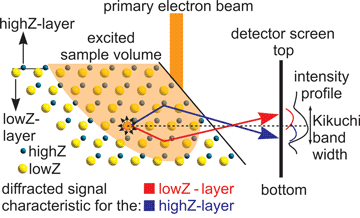
The illustration in Figure 3 summarizes the principle of evaluating polar information from Kikuchi bands by comparing the extremes of a profile through the correlated Hough peak. It also enables to understand the assignment of lowZ- or highZ-layers to crystal faces or plane traces in maps of EBSD-scans. The “bottom” of a tilted sample in the SEM is usually the “top” of an EBSD-scan. Figure 3 shows the lowZ-layer in the sample positioned toward the bottom of the sample; hence the characteristic Kossel cone intensity, caused by the atomic numbers and structure factors, appears at the top of the Kikuchi band which has also been confirmed using etch pits in a GaP wafer (Nolze et al., Reference Nolze, Grosse and Winkelmann2015). It should be noted that “left” and “right” are also switched between the sample and the EBSP. It is thus necessary to geometrically invert the EBSP before it is possible to assign bands to structure components and features. During automated indexing, this is done using the calibration data established for each SEM.

Fig. 3. Illustration of how a non-symmetric signal (Kikuchi band) forms on the detector screen of an EBSD camera in an SEM from a polar (111).
Results and Discussion
Figure 4 presents two zincblende patterns containing distinct Kikuchi bands also known as “reflections” and obtained using an acceleration voltage of 10 kV. Here, polar 111-reflections and nonpolar 220-reflections are highlighted. The word “reflections” is subsequently no longer used as the meaning is clear by lack of brackets for these indices. The Figures 4a and 4b show the pure patterns while the Figures 4c and 4d contain indices and further elements necessary for evaluation. The 111 and 220 localized almost horizontally or vertically are partially highlighted with a short, thick white bar, representing their direction and thickness. The parallel dashed white lines highlight the positions of discernible band edges of higher orders. The center of each band is marked with a black line. The pairs of solid white lines parallel to the respective band mark the boundaries of the Hough-peak profile, i.e. the area over which the gray value profile perpendicular through the respective reflection was averaged. The directions of these profiles are highlighted by white arrows.

Fig. 4. (a,b) EBSD patterns of zincblende crystals acquired using a 10 kV acceleration voltage. They contain polar 111 and nonpolar 220. (c) Horizontal  $11\bar{1}$, vertical
  $\bar{2}20$, and (d) almost vertical
  $11\bar{1}$ as well as almost horizontal
  $2\bar{2}0$ highlighted for closer examination. Thick white bars mark the bandwidth and dashed white lines mark edges of higher order bands. The white arrows show the directions of the acquired Hough-peak profiles (superimposed onto the band in white) which represent the information between the thin white lines parallel to the related bands. The pattern center (PC) is marked with a white cross. Selected zone axes are indexed.
To discuss the asymmetry of the polar planes, it is helpful to focus on the details of the [112]-zone axis which is a common direction of the nonpolar  $( {\bar{2}20} )$ and the polar
  $( {11\bar{1}} )$. The [112]-zone axis is located at the intersection of the two black lines in the Figures 4c and 4d. In Figure 4c, the intensity maximum of the profile is slightly above the horizontal black centerline. The intensity maximum is slightly shifted to the left of the vertical centerline in Figure 4d. In contrast, neither the vertical
  $\bar{2}20$ in Figure 4c nor the almost horizontal
  $2\bar{2}0$ in Figure 4d show a discernible asymmetry when comparing the immediate environment adjacent to the respective centerlines. Using the description and markings in the Figures 4c and 4d, it is easy to see the symmetry properties in the pure patterns of the Figures 4a and 4b. The pattern center (PC) as given by the calibration is respectively marked by a white cross. As predicted by Nolze et al. (Reference Nolze, Grosse and Winkelmann2015), the intensity of the first order of the reflection is lower on that side of the band to which the intensity maximum is shifted. While this effect cannot be evaluated exactly by the naked eye, it can be seen at the vertical reflection in Figure 4b but not at the horizontal reflection in Figure 4a (and marked in Fig. 4c).
The Figures 5a and 5b present the Hough transformation results of the EBSPs in the Figures 4a and 4b, and the Hough peaks of the discussed bands are respectively highlighted. Unfortunately, the vertical bands least affected by excess and deficiency effects are located at the boundaries of the Hough space, i.e. they are split into two parts near ρ = 0° and ρ = 180°. While it is possible to expand the Hough space, combining the two parts by inverting the ρ-scale of one and adding it to the other, this is not included in the commonly used Hough transformation. Hence, the obviously larger part which probably contains the center of the divided Hough peak is taken into account to create the respective profile for evaluation here. These profiles and details of the Hough peaks are discussed in Figure 6.

Fig. 5. Hough transformation of the patterns in the Figures 4a and 4b. The Hough peaks of the bands discussed in the Figures 4c and 4d are indexed. The BPS for the Hough transformation was 240 and no convolution mask was applied.

Fig. 6. Detailed analysis of the Hough peaks highlighted in Figure 5 using several Hough transformation settings, i.e. a BPS of 240 or 120 and a convolution mask of 0 × 0 or 9 × 9. The respective peak profiles are shown, passing vertically through the center of the Hough peaks from top to bottom. Gray scale values of the 1st minimum, the maximum, and the 2nd minimum are stated.
Figure 6 compares the averaged band profile with the profiles of the related Hough peaks resulting from the respectively stated Hough transformation settings. The profiles of the same band are shown along each column where the top profile presents the averaged profile taken directly from the EBSP. As introduced in Figure 2, the averaged profile transects the Kikuchi band perpendicularly from top to bottom just as the corresponding Hough peak profile transects the Hough peak from top to bottom. The dashed aid line highlights the slight shift of the profile maximum from the center toward one side.
The profile shapes within a column are very similar. The signs of the differences between the 1st and 2nd minimum also qualitatively match at a first glance within a column. The averaged profile of the horizontal  $11\bar{1}$ shows small oscillations near the minimum due to the higher orders of the band, which appear as dark lines parallel to the band in the Figures 4a and 4c. These oscillations also appear in the Hough peak profile at a BPS of 240 without a convolution mask (0 × 0) but disappear when using the BPS of 120 because the Hough peak profiles become smoother. The BPS influences the Hough peak length, i.e. the number of pixels between the minima. The higher resolution at a larger BPS directly leads to a larger ρ-scale and therefore to a longer Hough peak, but this only has a marginal effect on the profile shape.
This comparison is also valid for the vertical  $11\bar{1}$ and
  $\;\bar{2}20$. The horizontal
  $2\bar{2}0\;$forms an exception because of the far-range environment of the band within the EBSP presented in the Figures 4b and 4d, which is very asymmetric perpendicular to the profile direction. By contrast, the environment of the horizontal
  $11\bar{1}$ in the Figures 4a and 4c is almost symmetric. The EBSP details become increasingly distorted with an increasing distance from the PC, i.e. angles and bandwidths in the projection become increasingly deformed. The Hough transformation, as it is a line detection algorithm, rather describes the environment close to a line. Hence, the Hough peak profile shape of the horizontal
  $2\bar{2}0$ in Figure 6 is more similar to the averaged band profile and the Hough peak profiles of the vertical
  $\bar{2}20$ than to its related averaged band profile.
Applying the convolution mask leads to differences between the averaged band profile and the Hough peak profile. For example, comparing the shapes and signs of the differences between the 1st and 2nd minimum along each column shows that they qualitatively differ. The strongest deviations occur for the Hough peak profiles of the horizontal  $11\bar{1}$ and
  $2\bar{2}0$ using a BPS of 240. In the case of the
  $11\bar{1}$, the sign of the difference clearly becomes negative, which is in agreement with the impression that the sign becomes −1, i.e. zero considering the margin of error outlined in section “Theoretical effect of polarity on EBSPs and the Hough transformation,” for the
  $2\bar{2}0$. Furthermore, the profiles of the two 220 contain artifacts such as subpeaks when a BPS of 240 is used along with the 9 × 9 convolution mask. The convolution mask of the TSL software was developed and optimized to locate discrete peak positions, including those from bands with broad, flat inner band intensities. As a larger convolution mask includes more neighboring points, it can avoid the sub peaks in the Hough space resulting from broad, symmetrical bands.
The Figures 7a and 7b show two EBSPs of opposing crystal orientations and respectively inverse polarity effects recorded with an acceleration voltage of 5 kV. The bands are indexed in the illustrations of these patterns presented in the Figures 7c and 7d. Each pattern contains Kikuchi bands of three polar {111} and three nonpolar {220}. The intersections of the 220 mark the position of the <111>-zone axes. Polar 111 are illustrated in white with differing band edges (dark and bright gray), while the nonpolar 220 are illustrated in black only. The band edge contrast and the lowZ- or highZ-layers in the illustrated polar bands are defined arbitrarily. While diffraction from the highZ-layer of the polar bands is directed toward the  $[ {\bar{1}\bar{1}\bar{1}} ]$-zone axis in Figure 7c, the diffraction from the lowZ-layer is directed toward the [111]-zone axis in Figure 7d.

Fig. 7. (a,b) EBSPs of sphalerite crystals recorded using an acceleration voltage of 5 kV. (c) Indexed scheme of pattern (a) showing three 111, three 220, and the  $[ {\bar{1}\bar{1}\bar{1}} ]$-zone axis. (d) Indexed scheme of pattern (b) showing three 111, three 220, and the [111]-zone axis.
The Figures 8a and 8b present the Hough transformations of the EBSPs shown in Figure 7; the labeling of the subfigures and the indexing is consistent with Figure 6. The BPS was set to 120 and a 9 × 9 convolution mask was applied. The subfigures present enlarged sections of the indexed Hough peaks as well as the related profiles which are normalized in height and transect the peaks perpendicularly from top to bottom. The non-normalized absolute values of their extremes are displayed in a gray scale value range from 0 to 255. Comparing the differences between the 1st and 2nd minimum for polar and nonpolar bands enables the estimation of the excess and deficiency effects and deduce the EBSP polarity information.

Fig. 8. (a,b) Hough transformations of the EBSPs respectively presented in Figures 7a and 7b along with the same peak indices. A 9 × 9 convolution mask was applied. The respective normalized peak profiles are presented along with the gray scale values of the respective 1st minimum, the maximum, and the 2nd minimum.
Thus, it is possible to attribute the brighter and darker profile side of each Hough peak to the bands in the original EBSP. For a better understanding, this is done in the Figures 7c and 7d, which show the EBSP schematics. The Hough peaks of the nonpolar 220 appear to be symmetric in Figure 8. Regarding their profiles, the differences between the 1st and the 2nd minimum are −1, 8, and 14 in Figure 8a and −1, 13, and 17 in Figure 8b. A value of −1 can be interpreted as 0 considering the margin of error, see section “Theoretical effect of polarity on EBSPs and the Hough transformation,” and implies a symmetrical contrast of the top and bottom edge of the corresponding band. Instead, the positive differences show asymmetries which are caused by excess and deficiency effects in agreement with the literature (Schwartz et al., Reference Schwartz, Kumar, Adams and Field2009: 31). Excess effects with a high intensity appear bright at the top edge of a band, while deficiency effects appear dark at the bottom edge. By contrast, the Hough peaks of the 111 clearly appear to be asymmetric. Regarding their profiles, the differences are 36, −16, and 23 in Figure 8a and 34, −9, and 28 in Figure 8b.
The positive differences of the polar 111 are clearly stronger than in the case of the nonpolar 220. In both patterns, clearly negative differences only appear for two 111, i.e.  $\bar{1}\bar{1}1\;$in Figure 8a and
  $11\bar{1}$ in Figure 8b. These bands are almost horizontal in the EBSPs of the Figures 7a and 7b and the corresponding Hough peaks are clearly darker at their top than at their bottom. Although these two bands are actually those most affected by excess and deficiency effects, the difference is negative, which is opposite to the known effect of excess or deficiency effects. Therefore, a negative difference is a strong indicator for a band with the dark band edge at its top. Correlating the measured contrasts with the orientations of the bands in the EBSP shows that the bright minimum points toward the [111]-zone axis in the Figures 7a and 7c while the dark minimum points toward the
  $[ {\bar{1}\bar{1}\bar{1}} ]$-zone axis in the Figures 7b and 7d.
In order to assign the lowZ- and highZ-layers to the Kikuchi band edges and corresponding Hough peaks, it is necessary to consider the shift of the intensity maximum away from the Kikuchi band center. In the case defined in this study, the highZ-layers face heavier Zn-atoms while lowZ-layers face the lighter S-atoms. According to the relation described by Nolze et al. (Reference Nolze, Grosse and Winkelmann2015), the shift of the intensity maximum is directed from the band center toward that side which represents the layer facing the lighter atoms. As shown in this study, the band edge nearer to the shifted intensity maximum appears darker because of the lower minimum. Hence, the darker band edge, i.e. the lower Hough peak minimum, represents that layer which faces the lighter atoms, i.e. in this case the layer of S atoms.
Figure 9 presents four EBSPs recorded from the same crystal orientation featured in Figure 7d but obtained with acceleration voltages of 5, 10, 20, or 30 kV. The working distance was increased from 15 to 17 mm for the 30 kV pattern in order to keep the focus on the sample surface, causing a slight but discernible shift in the pattern of Figure 9d. All four EBSPs contain the same Kikuchi bands but, in agreement with the Bragg equation, the bandwidths of identical bands decrease with an increasing voltage. The band indexing is stated in Figure 9a as this pattern is already presented in Figure 7b. Paying special attention to the <112>-zone axes in the 111 enables to discern that the intensity maxima are visibly shifted toward the [111]-zone axis in all four patterns.

Fig. 9. (a–d) EBSPs of the same sphalerite crystal featured in Figure 7b acquired using the respectively stated acceleration voltages. The Figures 9e–9h show the respective Hough transformations superimposed by the indexed zone axes. The gray scale values of the peak extremes for each hkl are stated in the order: 1st minimum, maximum, 2nd minimum.
The Hough transformations of these patterns are presented in the Figures 9e–9h along with the values of the peak extremes for each indexed zone axis. The differences between the 1st and 2nd minimum of each peak are stated in Table 1. A constant Hough transformation setting with a BPS of 120 and a convolution mask of 9 × 9 was applied during analysis. For acceleration voltages of 5 to 20 kV the differences for the  $1\bar{1}\bar{1}$,
  $\bar{1}1\bar{1}$ and
  $\bar{2}20$ decrease while they increase for the
  $11\bar{1}$ and
  $\bar{2}02$. These trends are respectively broken in the patterns acquired using 30 kV, which is probably an effect of the geometrically necessary shift in the working distance noted above. The differences for the
 $\;02\bar{2}$ increase from 5 to 10 kV but decrease from 10 to 20 and 30 kV.
Table 1. Differences Between the 1st and 2nd minimum of the Hough Peaks Shown in the Figures 9e–9h

These trends show that increasing voltages have a negative effect on polarity evaluation as they tend to lead to positive differences between the 1st and 2nd minimum, possibly causing systematic errors. They also show that evaluating a single polar band can be insufficient for analysis, meaning as many polar bands as possible should be included into the analysis of the polarity. Furthermore, the optimal setup for polarity analysis using the Hough Transformation may vary and should be determined individually. For the setup applied here, an acceleration voltage of 30 kV is too high to provide a reliable analysis.
As the position of the measured crystal had to be adapted to the changed focus after each voltage modification, the EBSPs are shifted in height on the detector screen as the voltage is increased. This means that the electrons contributing to the respective bands were scattered with larger angles which modifies the intensity of excess and deficiency effects. The broader Kikuchi bands resulting from the lower acceleration voltages lead to an advantageous spread of the Hough peak profiles over the pixels of the detector in the EBSD camera. At higher acceleration voltages, the thinner bandwidth reduces the discernability of excess and deficiency effects, i.e. a line/effect may become thinner than one pixel is wide if the voltage is high enough. Simultaneously, the intensity of the excess and deficiency effects themselves is increased. Hence, the physical resolution of the used EBSD camera is a significant aspect to these measurements.
In summary, the results presented above show that the effect of the polarity on the Kikuchi band symmetry can be measured using the Hough transformation in the case of cubic ZnS. Recent studies showed that different atoms in the lowZ- and highZ-layers of polar planes lead to Kossel cones with characteristic asymmetric intensity distributions (Nolze et al., Reference Nolze, Grosse and Winkelmann2015; Winkelmann & Nolze, Reference Winkelmann and Nolze2015). This results in asymmetric Hough peaks in the Hough transformation of an EBSP. Evaluating the gray scale value relation between the minima beside the actual Hough peak in the Hough transformation can enable to deduct the existence of a polarity. Because the asymmetry shift depends on the atomic numbers of the involved atoms in the lowZ- and highZ-layers but not on the charge of their ions, it is not possible to determine the absolute polarity directly using the EBSP alone. If the chemical composition of the phase is known, Z can be included by attributing the lowZ- and highZ-layers of a polar plane. Then it is possible to assign the side of the lower Hough peak minimum to the layer that faces the lighter element. A reference method is useful for calibration, but the characteristic intensity shift caused by the atomic numbers has been proven for several similar materials. Hence the gray scale value profiles are sufficient for polarity determination if the exact chemical composition is known.
The ability to acquire this information from the Hough transformation means that it should be possible to determine non-centrosymmetric point groups during automated EBSD scans and produce, e.g. polarity maps for the analyzed area. In order to generalize the results, it is necessary to optimize the signal and consider all possible non-centrosymmetric crystal structures while regarding the diversity of all possible crystal orientations.
Such polarity maps are important, e.g. to the case of fresnoite glass-ceramics (Wisniewski et al., Reference Wisniewski, Thieme and Rüssel2018) which show not only an orientation selection but also a polarity preference during surface crystallization in glasses. While the piezoelectric activity of these materials proves that one polarity must be preferred over the other at some point, it is currently unknown whether this preference is significant during oriented nucleation (Wisniewski et al., Reference Wisniewski, Nagel, Völksch and Rüssel2010; Wisniewski & Rüssel, Reference Wisniewski and Rüssel2021) at the surface or during the subsequent growth into the bulk. Polarity maps obtained by EBSD at the immediate surface and at parallel cross-sections further in the bulk would answer this fundamental question in glass crystallization.
The present study shows that multiple parameters influence the discernibility of the polarity information. Acceleration voltage and Hough transformation settings such as the BPS and the convolution mask can spread or shrink the bandwidth details. The acceleration voltage additionally affects the intensity of the disturbing excess and deficiency effects. Hence, it may not be possible to directly obtain the layer assignment correctly for every pattern although it can be indexed in standard analysis. One solution for this problem could be a reduction of the excess and deficiency effect intensity by choosing a low acceleration voltage and a matching parameter set for the Hough transformation. In the case of cubic ZnS, it is advantageous to obtain patterns using 5 kV and to set the Hough transformation to a BPS of 120 and a convolution mask of 9 × 9.
However, considering only one polar band may be misleading, even if the signal has been optimized. A single Hough peak can directly and correctly be interpreted if the asymmetry caused by the Z difference between the lowZ- and highZ-layer is opposite to and stronger than the effect of the excess and deficiency effects. This is certain when the Hough peak is not split and the 1st minimum of a Hough peak is lower than the 2nd. Currently, all other cases need further consideration. Generally, only one or two of the strongest polar bands in an obtained EBSP will be considered for these evaluations. If the crystal structure/EBSP contains two or three polar planes/bands, the orientation relation between the polar bands can be used to evaluate the reliability of the peak profile asymmetries as discussed for the Figures 7a and 7b. Bands approaching verticality in a centered position yield the clearest results. As in these figures, any three 111 surrounding a <111>- zone axis face each other with the same layer type.
To produce reliable results from the Hough peaks of just one polar band, or several bands partially affected by polarity, it could be useful to develop a correction factor based on the nonpolar bands in an EBSP, which reduces the role of the excess and deficiency effects. Such a factor could be calculated as a function of the band width, band position, and band orientation. Furthermore, the acceleration voltage, the working distance, the position of the PC, and the phase composition should be included as parameters. As the detected EBSP is a result of all stated parameters, one quick approach could be to take the intensity of the excess and deficiency effects from Hough peak profiles of the indexed nonpolar bands. In the case of an automated scan, the profile correction factor could be calculated from a background pattern before scanning. This can then be used for all patterns of the same phase during a single scan.
Even an exactly vertical band orientation in the EBSP produces split peaks in the standard Hough transformation and may cause errors during the asymmetry determination. A potentially promising solution, applicable even after performing the peak localization algorithm, could be a mathematical extension of the Hough space boundaries with the data from the opposite Hough space boundary for peaks near the boundary.
Currently, the Hough peak evaluation method cannot be used during automated indexing before the suggested corrections have been developed. Nevertheless, it is possible to use the Hough peak profile evaluation to determine the absolute polarity on single EBSPs in the special case of single crystals or polycrystalline samples with preferred orientations if the phase is known.
Conclusions
Recording EBSPs of non-centrosymmetric crystal structures and their subsequent Hough transformation in the standard indexing procedure enables to determine the presence of polarity in a crystal, i.e. to distinguish the non-centrosymmetric point groups. Different atomic numbers between the lowZ- and highZ-layers of the polar planes can lead to asymmetric peaks in the Hough transformation if the Z-difference is large enough. These asymmetries can be evaluated by grey value profiles. If the chemical composition of the phase is known, it is also possible to assign the lowZ- and highZ-layer as well as the absolute polarity of the lattice plane.
The chosen acceleration voltage and Hough transformation settings clearly affect the applicability. In the case of ZnS, a comparably low acceleration voltage of 5 kV in combination with a BPS of 120 during the Hough transformation and the application of a 9 × 9 convolution mask is favorable in order to enable conclusions concerning the presence of a polarity and its orientation in the given experimental setup. Information on the polarity of a crystal and the location of polar axes should be helpful to determine the point group from an EBSP and to clarify crystallization mechanisms, e.g. during the CVD of ZnS or the surface crystallization of a polar phase in glasses.
Financial support
This work was funded by the Bundesministerium für Wirtschaft, BMWI (ZIM Program No. KF2519702FK1).


 Open access