


Impact Statement
The offshore oceanic atmospheric boundary layer is a special region for air–sea–land interactions, where flux transport is significantly affected by turbulent exchange in addition to weather processes. But the turbulent exchange process is more complicated because the offshore ocean atmospheric boundary layer, especially the coastal area atmospheric boundary layer, is affected by the land and sea-surface change, the coastal complex terrain and so on. During the turbulent gradient observation, a lot of valuable experimental data have been obtained. Combined with data analysis, our understanding of the offshore marine boundary layer has been further enhanced. Under a complex terrain, the vertical advection transport effect of the momentum in the marine boundary layer is very obvious. Due to the influence of the mountain terrain, the large vortex flux often affects the turbulent flux, resulting in an uncertainty of the turbulent flux.
1. Introduction
Turbulent heat fluxes between the ocean and the atmosphere and ocean surface wind stress influence weather and climate, and the state variables used to estimate them are essential both as ocean variables and climate variables (Reference Cronin, Gentemann and EdsonCronin et al., 2019). Wind stresses, i.e. air–sea momentum fluxes, are usually parameterized using the drag coefficient or roughness height, and they are related to wind speed at 10 m height, wave age, wave steepness, wave velocity, swell and so on (Reference CharnockCharnock, 1955; Reference DonelanDonelan, 1990; Reference Drennan, Graber, Hauser and QuentinDrennan, Graber, Hauser, & Quentin, 2003; Reference GeernaertGeernaert, 1987; Reference Johnson, Hojstrup, Vested and LarsenJohnson, Hojstrup, Vested, & Larsen, 1998; Reference Lange, Johnson, Larsen, Hojstrup, Kofoed-Hansen and YellandLange et al., 2004; Reference Smith, Anderson, Oost, Kraan and MaatSmith et al., 1992; Reference StewartStewart, 1974; Reference Taylor and YellandTaylor & Yelland, 2001; Reference Toba, Iida, Kawamura, Ebuchi and JonesToba, Iida, Kawamura, Ebuchi, & Jones, 1990; Reference WuWu, 1980; Reference Yelland and TaylorYelland & Taylor, 1996). However, the drag coefficient used in models always carries large error at high wind speeds, especially over coastal water (Reference Bi, Gao, Liu, Liu, Song, Huang and LiuBi et al., 2015; Reference Song, Chen, Wang, Zhi and LiuSong, Chen, Wang, Zhi, & Liu, 2016; Reference Zhao, Liu, Li, Dai, Song and LvZhao et al., 2015). In coastal regions, due to the complicated terrain and the sea–land boundary, the momentum flux cannot simply be parameterized as a variable and composited with multi-scale vortex components (Reference Cheng, Wu, Song, Wang and ZengCheng, Wu, Song, Wang, & Zeng, 2014, Reference Cheng, Huang, Wu and Zeng2015). The drag coefficient over the land footprint is significantly greater, by as much as an order of magnitude, than that over a smooth sea-surface footprint (Reference Grachev, Leo, Fernando, Fairall, Creegan, Blomquist and HocutGrachev et al., 2018).
Multi-scale flow structures are obvious phenomena in atmospheric turbulence. The characteristic form of the fluctuation (at a spatial scale from tens of metres to several hundred) has geometric and dynamic properties. Large-scale coherent structures organize and interact with small-scale pulsations and retain their characteristic form (Reference WilczakWilczak, 1984). During a recording of the atmospheric boundary layer temperature curve in 1958, it was found that the temperature periodically increased slowly over time and then suddenly decreased (Reference TaylorTaylor, 1958). Since then, many scientists have further observed and studied this phenomenon, and found that all the variables for turbulence exhibit organized large-scale motion. This coherent structure is manifested in temperature pulsation, with an obvious slope-like structure, sometimes called the slope structure of temperature (or ramp). It has also been found that wind-speed pulsation often has a strong upward ejection and downward sweeping motion, and forms a streak-like structure in wall turbulence. In recent years, it has been gradually recognized that a coherent structure is a common phenomenon in the atmospheric boundary layer (Reference Cheng, Huang, Wu and ZengCheng, Huang, Wu, & Zeng, 2015; Reference Cheng, Zeng and HuCheng, Zeng, & Hu, 2011; Reference Guala, Metzger and McKeonGuala, Metzger, & McKeon, 2011; Reference Hutchins and MarusicHutchins & Marusic, 2007; Reference Marusic, Mathis and HutchinsMarusic, Mathis, & Hutchins, 2010; Reference Zeng, Cheng, Hu and PengZeng, Cheng, Hu, & Peng, 2010; Reference Zheng, Zhang, Wang, Liu and ZhuZheng, Zhang, Wang, Liu, & Zhu, 2013), and the most recent of these studies have revealed that this coherent structure is multi-scale and interactive. Reference JimenezJimenez (2018) concluded that coherent streaks are the dominant flow structures within the buffer layer. Furthermore, an investigation into high Reynolds number experiments and simulations also revealed the formation of large-scale and very-large-scale motions residing in the log region (Reference Smits, McKeon and MarusicSmits, McKeon, & Marusic, 2011). Indeed, investigations of such data have progressively led to novel developments and questions about the interaction between small-scale turbulence and large-scale motions. Reference Hutchins and MarusicHutchins and Marusic (2007) provided further evidence of an amplitude modulation phenomenon via the large-scale motions residing in the log region on the near-wall (small-scale) dynamics. Reference Lotfy, Abbas, Zaki and HarunLotfy, Abbas, Zaki, and Harun (2019) examined the influence of atmospheric stability on the properties of turbulent coherent structures, and the monotonic increase in the energy content in the convective direction resulted in an enhanced modulating effect for the large super-streaks on the small vortex packets.
It has been found that the flux contribution rate of turbulent coherent structures is 37 %–45 % (Reference Lu and FitzjarraldLu & Fitzjarrald, 1994), and that 90 % of the transport can even be due to turbulent coherent structures (Reference Bergström and HögströmBergström & Högström, 1989), although these values may only be a special case observed over the short term (1–2 h). More and more studies have noted the limitations of Monin–Obukhov similarity theory (MOST) and found that turbulent coherent structures dominate the turbulent mixing process, and that MOST does not describe these structures well (Reference Gerbi, Trowbridge, Edson, Plueddemann, Terray and FredericksGerbi et al., 2008; Reference Sun, Mahrt, Nappo and LenschowSun, Mahrt, Nappo, & Lenschow, 2015, Reference Sun, Lenschow, LeMone and Mahrt2016). When mesoscale flow interacts with a complicated terrain, multi-scale turbulent coherent structures may be produced (Reference Smeets, Duynkerke and VugtsSmeets, Duynkerke, & Vugts, 1999, Reference Smeets, Duynkerke and Vugts2000). Many observations have shown that the relationship between friction velocity and average wind speed can easily fail at low wind speeds, wherein the constant flux layer near the sea surface is often destroyed and the momentum flux diverges (Reference Mahrt, Miller, Hristov and EdsonMahrt, Miller, Hristov, & Edson, 2018). Due to the influence of the coastline or topography, the surface stress is more easily dispersed. An increasing number of studies have found that MOST is not applicable in the marine boundary layer, and our study shows that the effect of multi-scale turbulent coherent structures on flux transport is more significant in the coastal boundary layer. Indeed, it has been suggested that a new hypothesis should be applied to the theory of the coastal boundary layer (Reference Sun and FrenchSun & French, 2016).
In this paper, the temporal and spatial characteristics of the multi-scale flow structures of the coastal boundary layer are analysed by observing data from different altitudes and different weather processes, which provides a basis for studying the flux relationship with complex coastal terrain.
2. Experimental site and equipment
The offshore ocean atmospheric boundary layer turbulence exchange observation experiment was carried out in Shenzhen Offshore Marine Boundary Layer Observation Station from 1 September to 20 October 2019 (Reference Zheng, Sun, Luo, Cheng, Shao, Zheng and LiuZheng et al., 2023). It is located off the southeast coast of Shenzhen Dapeng South Peninsula, northwest of where the peninsula is connected to the mainland. It is a mountainous peninsula, 700–800 m above sea level (a.s.l.). The highest mountain – Seven Niang Mountain – is 867 m a.s.l. The vegetation comprises subtropical grassy slopes, evergreen broadleaf forest and Masson pine forest. The coastline twists and turns, with a small total beach area and only a few beaches in the southwest (figure 1a). Yangmeikeng Environmental Ecological Centre is located half-way up the northeast coast of the peninsula (22°32′31.1′′N, 114°35′15.46′′E; 70 m a.s.l.) and the flux tower is positioned on its southern mountain, about 210 m away (22°32′24.77′′N, 114°35′14.03′′E; 130 m a.s.l.) (figure 1b). An ultrasonic anemometer (100 Hz, Model UAT-3, Institute of Atmospheric Physics, Chinese Academy of Science) and a water vapour carbon dioxide analyser (20 Hz, Model Li-7500A, LiCor Inc., Lincoln, Nebraska, USA) were set up on the 0.5 m long boom pointing to the east, mounted on the mast on the north side of the roof of the ecological centre and 20.8 m above the ground (figure 1e). The surface gradient toward the south and west is 14 %. The building is about 15 m high, and along with its neighbouring pathway covers approximately 50 × 50 m2. Around the centre are evergreen broadleaf trees that are approximately 5–6 m tall, which is less than 3 % of the minimum fetch (estimated to be 290 m) and therefore will not affect the flow; however, in the direction of land wind from 82° to 306°, because of the elevation of the terrain, the flow will be affected. The roughness is 0.27 m and the displacement is 14.37 m (figure 1d). Another set of equipment was set up on the 0.5 m long boom pointing to the north, which was mounted on the flux tower on the 14 % slope of the mountain at 13.9 m above the ground. There is a small platform under the tower free of vegetation. There are evergreen broadleaf trees approximately 5–6 m high along the slope that are less than 6 % of the minimum fetch, estimated to be 98 m, which will not affect the flow; however, in the direction of land wind from 75° to 310°, because of the elevation of the terrain, the flow will be affected. The roughness is 0.87 m and the displacement is 6.46 m (figure 1f–h). An ultrasonic anemometer was installed on the 0.5 m long boom pointing to the south, mounted on a frame at Sai Chung Gulf on the southwest of the peninsula (22°29′4′′N, 114°32′49′′E, 5.7 m a.s.l.) (figure 1c). The lattice structure of the frame and the distance from the ultrasonic anemometer to the frame were both designed to avoid disturbance to the flow. The maximum tide during the experimental period was 0.2 m and the minimum was 0.02 m. The beach is 2.6 km long and 40 m wide, and the frame is situated in the corner of the Gulf. It is in the water during maximum tide, 10 m from the beach, whereas it is on the beach during minimum tide. From 130° to 240°, the wind is onshore, but otherwise it is offshore. The minimum fetch is 105 m. The roughness is 0.006 m and the displacement is 4.11 m (figure 1i). The UAT-3 uses an array of transducers arranged on non-orthogonal axes. Three transducer pairs composed of three sonic paths are orientated at an elevation angle of ϕ = 45° to the horizontal plane with an azimuthal angle of θ = 120° between each path and with a path length between transducers of 15 cm. The observational range of the wind speed is 0–45 m s−1, and the resolution is 0.01 m s−1. An inclinometer is installed on the mounting base of each ultrasonic anemometer. The pitch, yaw and roll angles of the acoustic array of the ultrasonic anemometer are measured synchronously. The sampling frequency is 100 Hz.

Figure 1. Observational and experimental sites: (a) terrain of Shenzhen Dapeng South Peninsula; (b) source areas calculated using the footprint model of Reference Hsieh, Katual and ChiHsieh et al. (2000), in which the red contour represents the accumulated flux footprint on the site roof and the yellow contour represents the footprint on the site tower; (c) footprint on the site beach; (d) Yangmeikeng Environmental Ecological Centre; (e) equipment on the roof of the centre; ( f) flux tower on the mountain; (g) flux tower; (h) equipment mounted on the tower; (i) ultrasonic anemometer installed in the Gulf.
3. Data and methods
The experiment was conducted from 1 September to 20 October 2019, in which period the data from 7 to 26 September were continuous. At the beginning, quality controls were performed on these data. Tests of absolute limits, given as the range of the realistic data based on specified limits (Reference Rebmann, Kolle, Heinesch, Queck, Ibrom and AubinetRebmann et al., 2012), spike-value tests, amplitude resolution tests, dropout tests, higher-moment statistical tests and stationarity tests, were performed on the data, as described by Reference Vickers and MahrtVickers and Mahrt (1997). Then, the tilt angle of the instrument was measured with an inclinometer and corrected as in (3.1), and the coordinates were double rotated to calculate the flux (Reference Aubinet, Grelle, Ibrom, Rannik, Moncrieff and FokenAubinet et al., 2000)
 \begin{equation}\left. {\begin{array}{c@{}} {{v_1} = {v_0}\cos (\alpha ) + {w_0}\sin (\alpha
),}\\ {{w_1} = {-} {v_0}\sin (\alpha ) + {w_0}\cos (\alpha
),}\\ {{w_2} = {w_1}\cos (\beta ) + {u_0}\sin (\beta ),}\\
{{u_1} = {-} {w_1}\sin (\beta ) + {u_0}\cos (\beta ),}\\
{{u_2} = {u_1}\cos (\gamma ) + {v_1}\sin (\gamma ),}\\
{{v_2} = {-} {u_1}\sin (\gamma ) + {v_1}\cos (\gamma ),}
\end{array}} \right\}\end{equation}
\begin{equation}\left. {\begin{array}{c@{}} {{v_1} = {v_0}\cos (\alpha ) + {w_0}\sin (\alpha
),}\\ {{w_1} = {-} {v_0}\sin (\alpha ) + {w_0}\cos (\alpha
),}\\ {{w_2} = {w_1}\cos (\beta ) + {u_0}\sin (\beta ),}\\
{{u_1} = {-} {w_1}\sin (\beta ) + {u_0}\cos (\beta ),}\\
{{u_2} = {u_1}\cos (\gamma ) + {v_1}\sin (\gamma ),}\\
{{v_2} = {-} {u_1}\sin (\gamma ) + {v_1}\cos (\gamma ),}
\end{array}} \right\}\end{equation}
where u 0, v 0 and w 0 are the three components of the original velocity which refer to longitude velocity, latitude velocity and vertical velocity; u 1, v 1 and w 1 are the three components of the first rotation velocity; u 2, v 2 and w 2 are the three components of the second rotation velocity which refer to streamwise velocity, spanwise velocity and vertical velocity; and α, β and γ are the roll, pitch and yaw angles, respectively. Averaging the wind speed for half an hour gives the ‘mean flow’ ( $\bar{u}_0,\bar{v}_0,\bar{w}_0$) and (
 $\bar{u}_2,\bar{v}_2,\bar{w}_2$), the wind direction is defined as
 \begin{equation}WD = \textrm{arctg}\left( {\frac{{\bar{v}_0}}{{\bar{u}_0}}} \right).\end{equation}
Replacing (u 2, v 2, w 2) as (u, v, w) and ( $\bar{u}_2,\bar{v}_2,\bar{w}_2$) as (
 $\bar{u},\bar{v},\bar{w}$), taking u for example, we have
 \begin{equation}u = \bar{u} + u^{\prime}.\end{equation}
Usually, the departure of instantaneous wind from mean velocity, i.e. u′ is called as fluctuation or turbulence. The Obukhov length L is a characteristic quantity obtained by integrating ground momentum and heat turbulence information, and z/L is the stability which can be calculated as follows:
 \begin{equation}\frac{z}{L} = {-} \frac{{z\kappa g\overline {w^{\prime}\theta ^{\prime}} }}{{u_\ast ^3\bar{\theta }}},\end{equation}
where z is measurement height, κ is von Karman constant, which usually is 0.4, g is gravity accelerated velocity,  $\overline {w^{\prime}\theta ^{\prime}}$ is sensible heat flux,
  $\bar{\theta }$ is potential temperature, the bar represents the average of one half an hour. Here, u * is friction velocity
 \begin{equation}
{u_{_\ast }} \equiv \left[\overline{{(u^{\prime}w^{\prime})}}^2 + \overline {(v^{\prime}w^{\prime})}^2\right]^{1/4}.\end{equation}
\begin{equation}
{u_{_\ast }} \equiv \left[\overline{{(u^{\prime}w^{\prime})}}^2 + \overline {(v^{\prime}w^{\prime})}^2\right]^{1/4}.\end{equation}
The turbulent energy e is calculated as follows:
 \begin{equation}e = {\textstyle{1 \over 2}}({\overline {{{u^{\prime}}^2}} + \overline {{{v^{\prime}}^2}} + \overline {{{w^{\prime}}^2}} } ).\end{equation}
We used an approximate analytical model based on a combination of Lagrangian stochastic dispersion model results and dimensional analysis to estimate the scalar flux footprint in thermally stratified atmospheric surface layer flows (Reference Hsieh, Katual and ChiHsieh, Katual, & Chi, 2000). The input parameters were as follows: sensor height,  ${z_s} = (z - {z_d})/{z_0}$, where z 0 is the roughness length and zd is the displacement height; a stability parameter, calculated as zs/L, where L is the Monin–Obukhov length; and friction velocity u *. The fetch, xF, which ensured that a particular observation height was still in the equilibrium layer fully adapted to upwind surface roughness, was affected by wind direction, stability and measurement height.
Then, we analysed the multi-scale characteristics with the wavelet transform and a finite element method based on bounded variation. A detailed introduction to these methods is given next and in the supplementary material available at https://doi.org/10.1017/flo.2023.24.
The wavelet transform, originally developed by Reference MorletMorlet (1981), has had a major impact in many areas of science and engineering. It can expand the time series into time–frequency space and find localized intermittent periodicities. The continuous wavelet transform (CWT) is well suited for feature-extraction purposes and is a common tool applied to analyse localized intermittent oscillations in a time series. According to the method of Reference Grinsted, Moore and JevrejevaGrinsted, Moore, and Jevrejeva (2004), we constructed the cross-wavelet transform from two CWTs, which revealed the wavelet coherence coefficient (WCC) and relative phase between two variables.
Because the wavelet function  ${\Psi _\textrm{0}}(\eta )$ is generally complex, the wavelet transform
  $W_n^X(s)$ is also complex. One can define the wavelet power spectrum as
  $|W_n^X(s){|^2}$. Here, η is dimensionless time, η = t/s, s is the wavelet scale.
To make it easier to compare different wavelet power spectra, it is desirable to find a common normalization for the wavelet spectrum. The expected value for  $|W_n^X(s){|^2}$ is equal to N times the expected value for
  $|{\hat{x}_k}{|^2}$, which is the discrete Fourier transform of
  ${x_n}$. For a white-noise time series with a flat power spectral density, this expected value is
  $\sigma _X^2/N$, where
  $\sigma _X^2$ is the variance. Thus, for a white-noise process, the expected value for the wavelet transform is given by
  $|W_n^X(s){|^2} = \sigma _X^2$ for all n and s.
The CWT has edge artefacts because the wavelet is not completely localized in time. It is therefore useful to introduce a cone of influence (COI) in which edge effects cannot be ignored. The COI is the region of the wavelet spectrum in which edge effects become important and is defined here as the e-folding time for the autocorrelation of wavelet power at each scale. This e-folding time is chosen so that the wavelet power for a discontinuity at the edge drops by a factor e −2 and ensures that the edge effects are negligible beyond this point.
The cross-wavelet transform of two time series  ${x_n}$ and
  ${y_n}$ is defined as
  $W_n^{XY} = W_n^XW_n^{Y\ast }$, where * denotes complex conjugation. Reference Torrence and CompoTorrence and Compo (1998) further defined the cross-wavelet power as
  $|W_n^{XY}|$. The wavelet coherence between the two series is the ratio between the real argument,
  $\textrm{real}(W_n^{XY})$, and
  $\sqrt {\left|W_n^X(s)\right|^{2}\left|W_n^Y(s)\right|^{2}}$.
4. Results and analysis
Figure 2 was the 30 min averaged velocity. The wind speed was low throughout the observation period. There was a gale on 21–22 September. In addition, there was a clear sea–land wind. There was a strong sea breeze during the day, with an accompanying updraft. At night, it was a weaker land wind, with vertical advection movement barely detectable. Analysis of the sea–land wind process, stable stratification and strong wind process was made at (i) 1300 LT (local time = UTC + 8 h) on 10 September during the sea-breeze period; (ii) 2200 LT on 11 September during the land-wind period; (iii) 1500 LT on 13 September during the sea-breeze to land-wind transition process; (iv) 0600 LT on 15 September during the land-wind to sea-breeze process; (v) 2300 LT on 18 September during nocturnal stable stratification; and (vi) 0500 LT on 21 September during strong winds.

Figure 2 Time series of (a) average horizontal velocity (solid lines with left ordinate) and vertical velocity (dashed lines with right ordinate) and (b) turbulent kinetic energy (solid lines with left ordinate) and friction velocity (dashed lines with right ordinate) at the three sites
4.1 Momentum flux
Cases 1–6 correspond to the yellow lines in figure 2. Table 2 shows the meteorological conditions and main turbulence parameters of these six processes. It can be seen from figure 2(a) that, during the sea-breeze period (cases 1, 3 and 6), strong vertical motion is shown at the roof and tower owing to the complex terrain of the underlying surface, and the wind shows an obvious updraft, which is more obvious on the roof of the monitoring station located half-way up the mountain. Although the altitude of the tower is higher than the roof, the level at which the equipment is mounted on the roof is higher than the tower, and the footprint range of the roof (approximately 2 km) is larger than the tower (approximately 1 km) (figure 1b). The wind at the roof is more affected by the terrain than the wind at the tower. During the land-wind process (cases 2, 4 and 5), the wind speed is low and the vertical velocity is almost zero. In case 6, there is a strong systematic northwest wind; wind speeds in all three layers increase; the flatter the terrain, the stronger the wind speed; and the rougher the terrain, the larger the vertical velocity.
Turbulent kinetic energy and friction velocity (figure 2b) are also stronger during the day (sea breeze) than at night (land wind). During the conversion processes, such as sea breeze to land wind (case 3), or vice versa (case 4), even during the land-wind period (case 5), the wind direction changes frequently, sometimes being the sea breeze and sometimes the land wind, and the turbulent kinetic energy and friction velocity change irregularly from day to night. The turbulent kinetic energy and friction velocity increase obviously in windy weather (case 6). During this process, although at the Gulf it is a land wind, at the other two sites there are sea breezes, and the stronger wind at the Gulf produces stronger turbulence than the wind at the roof or tower.
From the wind-speed rose map (figure 3a–c), it can be seen that the main wind directions at the roof of Yangmeikeng Monitoring Station and at the Sai Chung Gulf site are sea-breeze and land-wind transformations, the former being from a northeasterly sea breeze to a southwesterly land wind, and the latter being from a southeasterly sea breeze to a northwesterly land wind. The wind direction at the mountain flux tower is highly complex as it is greatly affected by the terrain, and the sea breeze from northwesterly to northeasterly is strong, while the others are weak land winds.

Figure 3. Wind-speed rose at the (a) roof, (b) tower and (c) Gulf sites, and (d) the stability rose.
The stability rose diagram is obtained by using the stability  $z/L$ and friction velocity
  $u_\ast ^3$ (figure 3d). The abscissa is
  $u_\ast ^3$ and the ordinate is
  $(z/L)u_\ast ^3$, so their ratio is
  $z/L$, which can be converted to an angle to draw a stability rose diagram. Table 1 is the classification of stability. The contours indicate the magnitude of
  ${u_\ast }$. It can be seen that the average stability is weak instability, which is a common feature for the marine atmospheric boundary layer. However, for
  ${u_\ast } < 0.2\;\textrm{m}\;{\textrm{s}^{ - 1}}$, the stability is divergence because of the calculation error due to the small friction velocity.
Table 1. Classification of atmospheric stability

Table 2. Meteorological conditions and main turbulence parameters of the six processes.

From the analysis above we know that during sea-breeze periods the wind is strong and the friction velocity is large, while during the land-wind process the wind is weak and the friction velocity is small. Figures 4(a)–4(c) show the relationship between friction velocity and wind speed at the three sites. It can be seen that most land winds are weaker than sea breezes, but at the Gulf there are some particularly strong winds that happened during the strong weather process on 21–22 September. The drag coefficient (CD) is defined as the square of the ratio between the friction velocity and the mean velocity based on the log-law vertical profile of the mean velocity in the atmospheric boundary layer. The slopes in figures 4(a)–4(c) reflect that the root mean square of the drag coefficient is larger during land-wind periods than sea-breeze periods because of the complex terrain passed by the land wind. Figures 4(d)–4( f) show the relationship between the drag coefficient and wind speed at the three sites. The drag coefficient decreases with wind speed. At the same drag coefficient, the wind velocity is lower during land-wind than sea-breeze periods because it can produce turbulence even when wind velocity is very weak at the complex terrain, while cannot at the flat sea surface. However, the difference at the tower is not as obvious as at the other two sites because the terrain causes the wind direction to be complex (figure 3b), and the difference between sea breezes and land winds is unimportant.

Figure 4. Relationship between (a–c) friction velocity and wind speed and (d–f) CD and wind speed at the (a,d) roof, (b,e) tower and (c, f) Gulf sites.
4.2 Momentum flux of multi-scale flow structure
The wind directions and the footprints are different at the three sites. As expected, when the terrain is inhomogeneous, the structures of the vortexes are various. Therefore, the flux is decomposed into the contributions of different scale vortices by scale decomposition and divided into three main parts: the flux of turbulence of less than 1 min; the flux of gusts of between 1 and 30 min; and vertical advection transport by large-scale structures of over 30 min. Figure 5 shows that the contribution of larger-scale structures (30 min to 3 h) to the friction velocity is significant because of the mountainous topography. The sea surface of the Gulf is flat and the friction velocity due to turbulence of less than 1 min is dominant. And the total flux is always less than the sum of three parts of fluxes contributed by turbulence, gust and large-scale structure. Especially in the Gulf, when the wind speed is small during land wind, the total flux could be less than the turbulence flux due to the momentum flux diverging. Such a situation also appeared at the roof during the strong wind period of 21–22 September because the large-scale vortex had strong positive coherence (figure 9). At the roof, tower and Gulf, the averaged turbulence friction velocities are 0.22 m s−1, 0.22 m s−1, 0.16 m s−1, the averaged gust friction velocities are 0.31 m s−1, 0.31 m s−1, 0.12 m s−1, the averaged large-scale structure friction velocities are 0.32 m s−1, 0.31 m s−1, 0.13 m s−1 and the averaged total friction velocities are 0.49 m s−1, 0.5 m s−1, 0.24 m s−1.

Figure 5. Scale decomposition of friction velocity at the (a) roof, (b) tower and (c) Gulf sites.
Naturally, it could be assumed that the multi-scale structures also produce their drag coefficients. Figure 6 shows the drag coefficients of three scale structures. It can be seen that the variation in the drag coefficients of gusts and large-scale structures is more than that of turbulence. Due to the complex terrain at Yangmeikeng Monitoring Station and the tower on the mountain, it can be seen that the drag coefficient caused by gusts or large-scale structures is large and the sea–land conversion of wind is not as regular as at Sai Chung Gulf. Meanwhile, the Gulf has a flat underlying surface, and the drag coefficient caused by turbulence is much larger than that of the roof or tower. At the roof, tower and Gulf, the averaged turbulence CD values are 0.023, 0.024, 0.016, the averaged gust CD values are 0.033, 0.031, 0.012, the averaged large-scale structure CD values are 0.035, 0.032, 0.014 and the averaged total CD values are 0.074, 0.071, 0.028.

Figure 6. Value of CD at the (a) roof, (b) tower and (c) Gulf sites.
At the Gulf, the drag coefficient of turbulence shows obvious daily change, and is large at night during land-wind periods and small during daytime in sea-breeze periods. Figure 7 gives the drag coefficient and friction velocity due to turbulence alone and shows clearly that they both change regularly with the sea-breeze to land-wind conversion. However, the transformation is opposite in that the drag coefficient is small during daytime owing to the footprint being mainly flat sea surfaces, and large at night because of the rough terrain footprint when land winds blow. On the contrary, the friction velocity is large during daytime owing to the strong sea breeze and small at night for the weak land wind.

Figure 7. Values of CD and friction velocity due to turbulence at the Gulf site.
Figures 8(a)–8(c) show the relationships between friction velocity and wind speed of the three scale structures. At the roof, the drag coefficients represented by the slopes of different scale structures are almost the same, but the slope of total flux is obviously larger than the slope of anyone scale. At the tower on the mountain, the slopes of different scale structure are different because the coherences of the gust and large-scale structure are not strong due to an irregular change of wind direction. The fluxes of the gust and large-scale structures are larger than the flux of turbulence, but the increase of flux with their speed is less than that of turbulence. At the Gulf, the drag coefficient of turbulence is larger than the other two, and the slope of total flux is the same as that of turbulence, and larger than the other two scales, which means that the fluxes of the gust and large-scale structure are not important in the the flat terrain. Figures 8(d)–8( f) show the relationships between CD and wind speed of the three scale structures, revealing that all CD values decrease with wind speed. However, the relationship between the CD produced by gusts and wind speed is better than that of the others, especially at the Gulf. Because the wind speed is low during the experiment period, although the gust and large-scale structure contribute to the flux and affect the increase of flux with wind speed, the dynamic roughness is not changed, and the relationship between CD and wind speed is not changed.

Figure 8. Relationships between (a–c) friction velocity and wind speed and (d–f) CD and wind speed of three scale structures at the (a,d) roof, (b,e) tower and (c, f) Gulf sites.
4.3 Coherence of multi-scale flow structure
From the analysis above, we can see that the contributions of other scale structures except turbulence to the flux are also very obvious.
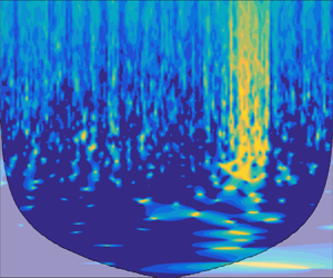
In this section, we mainly analyse the coherence of these structures. Figures 9–11 are the WCCs of the horizontal and vertical wind speed of the structures with scale between 1 min and 5 d. From the WCC, we can see that the large-scale vortex had strong negative coherence at the roof and Gulf due to the regular change of land wind and sea breeze, but positive coherence at the tower due to the irregular wind direction. However, during the strong wind period on 21–22 September, there were positive coherence vortices at the roof, while at the other two sites the characteristics of coherence were not obvious.

Figure 9. The WCC of the horizontal and vertical wind speed of the structures with scale between 1 min and 5 d at the roof site. The two red lines represent the scale of less than 30 min (gusts) and 3 h (large-scale structures), and the white lines are the average WCCs of the two scale structures.

Figure 10. Same as figure 9, but at the tower site.

Figure 11. Same as figure 9, but at the Gulf site.
In figures 9–11, the two red lines represent the scale of less than 30 min (gusts) and 3 h (large-scale structures), and the white lines are the average WCCs of the two scale structures. The WCCs of gusts at the roof and Gulf change regularly, while that at the tower changes irregularly, which agrees with the daily change of wind direction at the roof and Gulf, as well as the disorderly change in wind direction at the tower. The regular wind gusts at the roof and Gulf make the drag coefficient change consistently with wind speed (figures 8d and 8f). The coherence of large-scale structures is consistent with the coherence of gusts, because the large-scale structures interact with the small-scale structures at the roof (figure 9). This makes the fluxes contributed by turbulence, gusts and large-scale structures almost the same, and the slopes in figure 8(a) are very close. Meanwhile, at the Gulf, the WCC of large-scale structures somehow changes inconsistently with gusts (figure 11). It is perhaps the case that, at this site, the large-scale structures are produced by effects beyond the boundary layer because the height of the atmospheric boundary layer at the Gulf is lower than that at the roof.
5. Conclusion
The turbulent momentum fluxes of a flat underlying surface and complicated underlying surface were analysed by observations of coastal multilayer turbulence. The fluxes were related to wind speed, wind direction and the underlying surface. The friction velocities all increased with wind. However, during sea breezes they increased slowly and during land winds they increased rapidly, especially at the Gulf site where the underlying surface changes greatly during sea–land transition. Furthermore, under the usual calm weather conditions during the observation period, the wind speed was not large, so the CD value decreased with wind.
Besides those effects, it was found that the influence of the underlying surface produced a multi-scale structure, which had an obvious influence on momentum flux transmission. These multi-scale flow structures were affected by the underlying surface and behaved differently at different positions. The complex terrain can lead to a strong, negative coherence structure, which changes regularly with sea–land transition and yields interaction between large- and small-scale structures. However, when the wind direction is complex owing to the effect of terrain, such as on the mountain, the regularity and interaction disappear. On flat surfaces such as the beach, although there are multi-scale structures, turbulence bears no relationship with large-scale structures and makes greater contributions to flux than other scale structures.
Supplementary material
Supplementary materials are available at https://doi.org/10.1017/flo.2023.24.
Acknowledgements
We thank D. Harries for making available the Python code of BV-FEM and helping us to use the code successfully. We also thank Professor Z. She for the useful discussion, as well as S. Jia, H. Du and S. Zhou for completing the experiment successfully.
Declaration of interests
The authors declare no conflict of interest.
Funding statement
This work was supported by the National Key Research and Development Plan from the Ministry of Science and Technology of China under Grant 2018YFC0213102, the National Science Foundation of China under Grant 42175103 and the National Key Scientific and Technological Infrastructure project ‘Earth System Science Numerical Simulator Facility’ (EarthLab).
Author contributions
Q.L., S.Z., J.C., S.S. conducted experiments, performed analysis of results. L.Y. and M.Z. provided experiment conditions. H.Z. supervised the project. H.C. designed experiments. X.C. created the research plan and wrote the paper.


 Open access