

I. INTRODUCTION
This paperdevelops a number of tools and algorithms to analyze the sensor placement problem. The problem is formulated as an optimization problem where a limited number of sensors is placed to maximize an efficacy cost criterion. The solution involves solving an integer programming problem that becomes infeasible when the number of sensors and locations becomes large. The paper makes two key contributions; development of set of approximation algorithms (greedy algorithms and variations using the efficacy cost and also a projection-based method) that run in polynomial time in the number of parameters and derives a set of analytical nested performance upper bounds to the optimal solution based on the structure of the data correlation matrix. Simulations are conducted on a number of experiments from random correlation matrices, to a simulated sensor network, to an IEEE 57- bus test system [1] that show how tight the nested performance upper bounds are and that the approximation algorithms give lower bounds to the optimal solution that are close to the optimal solution.
Data gathering, data mining, or data analytics have become increasingly more important in a wide range of areas from energy to health care to social networking to business to the environment. The National Science Foundation recently had a call for proposals on “Big Data” to study these problems. An important part is how data are gathered which in many cases require using distributed sensor networks and monitors. In applications ranging from the electrical power grid to the natural environment to biomedical monitoring there is a need to deploy sensors to monitor and estimate the behavior of different complex systems. Often the number of sensors that can be deployed is limited by cost and other constraints (e.g. communication and energy constraints of the sensors).
There has been much previous work on the optimal placement of sensors. In Dhillon et al. [Reference Dhillon, Chakrabarty and Iyengar2, Reference Dhillon and Chakrabarty3] the optimal placement of sensors is considered where the probability of sensor detection depends upon distance with sensors placed on a two- or three-dimensional grid. Other research has considered sensor placement for the power grid by considering placement of phasor measurement units (PMUs) [Reference Chen and Abur4, Reference Xu and Abur5]. In their research the problem is formulated as a state estimation problem with PMU placement depending on a key condition to make the system observable. In [Reference Dua, Dambhare, Gajbhiye and Soman6, Reference Chakrabarti, Venayagamoorthy and Kyriakides7], the optimization criterion is to maximize the measurement redundancy while minimizing the required number of PMUs. To solve this problem, Dua et al. [Reference Dua, Dambhare, Gajbhiye and Soman6] considered the phasing of PMU deployment in an integer linear programming (ILP) framework, while Chakrabarti et al. [Reference Chakrabarti, Venayagamoorthy and Kyriakides7] took a binary particle swarm optimization (BPSO)-based approach. In work by Krause et al. [Reference Krause, Singh and Guestrin8] they model spatial phenomena as a Gaussian Process and consider placement of sensors again using optimal experimental design. The goal is to maximize mutual information and the problem again becomes a combinatorial optimization problem that is NP-complete. This paper also discusses a greedy algorithm and shows that mutual information is submodular and is monotonically increasing for small number of sensors. Performance bounds are obtained for the greedy algorithm. Simpler reduced computation algorithms and robust algorithms are also considered. More recently in [Reference Li, Negi and Ilić9], PMU placement is considered in a different context where observability is assumed and the goal is to optimize the experimental design using a different criterion. The solution involves solving an integer programming problem, which is NP-complete. However, an approximate greedy solution is found that gives good results and runs in polynomial time. Then the greedy algorithm is tied to submodular and monotonic functions where bounds can be obtained to the greedy algorithm in relationship to the optimal algorithm. An estimation-theoretic approach to the PMU placement problem is proposed in [Reference Kekatos and Giannakis10, Reference Kekatos, Giannakis and Wollenberg11]; after posing system state estimation as a linear regression problem, a convex relaxation is developed to suboptimally solve the PMU placement problem. In [Reference Bajovic, Sinopoli and Xavier12], the authors consider the sensor selection problem in a wireless sensor network for event detection, under two hypotheses – event occurring and event not occurring. They propose the maximization of the Kullback–Liebler and Chernoff distances between the probability distributions of the selected sensor measurements, under these hypotheses, as the optimization criteria. After proving that this problem is NP-hard, the authors propose a greedy algorithm as a general approach to solve this problem suboptimally.
We consider a static discrete optimization problem where we have n discrete node locations where we can deploy sensors and we have m sensors to place. The objective is to minimize the sum of the mean-squared error at all node locations. This has some close ties to [Reference Krause, Singh and Guestrin8, Reference Li, Negi and Ilić9] and has applications to energy problems. Examples include placement of meters such as advanced metering infrastructure (AMI) on the distribution grid or to deploy environmental resource sensors where distributed photovoltaic (PV) solar panels are located.
The optimization criteria we consider is also known as the A- optimality design of experiments maximizing the trace of the inverse of the information matrix also considered in [Reference Krause, Singh and Guestrin8–Reference Kekatos, Giannakis and Wollenberg11]. A key difference between this paper and the others is that here we consider a variety of computationally efficient approximation algorithms for the sensor placement problem and come up with analytical nested lower and upper bounds (depending on the structure of the correlation matrix) for the cost function of the optimal sensor placement. In [Reference Li, Negi and Ilić9], the authors present a bound on the optimal PMU placement problem under the assumption that the reward function is submodular. Under the submodularity assumption, the optimal solution is upper bounded by the greedy solution factored by e/(e − 1). This bound is usually not very tight, because it does not take the covariance matrix structure (i.e. eigenvalues, eigenvectors, etc.) into account. In contrast, we do not assume any submodularity condition and the upper bounds are obtained analytically in terms of the eigenvalues of the covariance matrix. This paper significantly extends work by the authors in [Reference Uddin, Kuh, Kavcic and Tanaka13, Reference Uddin, Kuh, Kavcic, Tanaka and Mandic14] by considering a broader array of approximation algorithms including projection-based algorithms, presenting nested upper performance bounds with a complete analysis of these bounds (based on matrix pencils, generalized eigenvectors, and matrix manipulations), and a more complete set of simulation studies.
Section II gives a formulation of the problem. Since the optimal solution is computationally difficult to obtain for large n and m, we present some approximation solutions and lower bounds to the optimal solution in Section III. These include the expedient solution, greedy algorithm, and an algorithm based on dynamic programming heuristics. Next, in Section IV we find a family of upper bounds to the optimal solution. In Section V, we present some more lower bounds based on the projections of the solution subspace that achieved the upper bounds in Section IV. In Section VI, we present simulation results for randomly generated data, a 5 × 5 grid model, and data generated from the IEEE 57-bus test system [1]. Finally, Section VII summarizes results of this paper and suggests directions for further work. In this paper, we do not present any iterative solutions, however, any of the approximate solutions presented can be used as a starting point of an iterative algorithm [Reference Crow15].
Notation
Upper and lower case letters denote random variables and their realizations, respectively; underlined letters stand for vectors; boldface upper case letters denote matrices, and I denotes the identity matrix; 〈·,·〉 denotes a matrix pencil; (·) T and E (·) stand for transposition and expectation, respectively.
II. PROBLEM STATEMENT
We assume that the state vector is X ∈ ℝ n and the observation vector is Y ∈ ℝ m where m ≤ n. Sensors are all identical and give noisy readings of the state, where the variance of each sensor reading is σ2. The model is described by
 $$\underline{Y} = {\bf C} \lpar \underline{X} + \sigma \underline{N}\rpar \comma \;$$
where
N
is a random vector with mean
0
and covariance matrix
 ${\bf \Sigma}_{\underline{N}} = {\bf I}_{n}$
with I
n
being an identity matrix of dimension n and
X
are random vectors with mean
0
and covariance matrix Σ
X
.
X
and
N
are jointly independent. C is a binary matrix with orthonormal rows, where each row has one ‘1’. In other words, C is composed of m rows of the n × n identity matrix I
n
. The positions of ones in the matrix C denote the position of the sensors.
${\bf \Sigma}_{\underline{N}} = {\bf I}_{n}$
with I
n
being an identity matrix of dimension n and
X
are random vectors with mean
0
and covariance matrix Σ
X
.
X
and
N
are jointly independent. C is a binary matrix with orthonormal rows, where each row has one ‘1’. In other words, C is composed of m rows of the n × n identity matrix I
n
. The positions of ones in the matrix C denote the position of the sensors.
The linear minimum mean-squared error estimator is given by [Reference Kay16]
 $$\hat{\underline{X}} \lpar \underline{Y}\rpar = {\bf E} \left(\underline{X} \, \underline{Y}^{T} \right){\bf E} \left(\underline{Y} \, \underline{Y}^{T} \right)^{-1} \underline{Y}.$$
The error is defined by
 $\underline{{\cal E}} = \underline{X} - \hat{\underline{X}} \lpar \underline{Y}\rpar $
and the error covariance matrix is given by [Reference Kay16]
$\underline{{\cal E}} = \underline{X} - \hat{\underline{X}} \lpar \underline{Y}\rpar $
and the error covariance matrix is given by [Reference Kay16]
 $${\bf E} \left(\underline{{\cal E}} \, \underline{{\cal E}}^{T} \right)= {\bf \Sigma}_{\underline{X}} - {\bf E} \left(\underline{X} \, \underline{Y}^{T} \right){\bf E} \left(\underline{Y} \, \underline{Y}^{T}\right)^{-1} {\bf E} \left(\underline{Y} \, \underline{X}^{T} \right)\comma \;$$
where
 $$\eqalign{{\bf E}\left(\underline{X}\, \underline{Y}^{T} \right)= {\bf \Sigma}_{\underline{X}} {\bf C}^T}\comma \;$$
and
 $$\eqalign{{\bf E} \left(\underline{Y} \, \underline{Y}^{T} \right)= {\bf C} {\bf \Sigma}_{\underline{X}} {\bf C}^{T} + \sigma^2 {\bf I}_{m}.}$$
Our task is to find the matrix C that minimizes the total error
 ${\rm tr} {\bf E} \left(\underline{{\cal E}} \, \underline{{\cal E}}^{T} \right)$
.
${\rm tr} {\bf E} \left(\underline{{\cal E}} \, \underline{{\cal E}}^{T} \right)$
.
Definition
Let
 ${\cal {C}}^{\lsqb m\times n\rsqb }$
denote the set of all m × n matrices composed of m rows of the identity matrix I
n
.
${\cal {C}}^{\lsqb m\times n\rsqb }$
denote the set of all m × n matrices composed of m rows of the identity matrix I
n
.
The optimization problem is then given by
 $${\bf C}^{\ast} = \mathop{\arg \min}\limits_{{\bf C} \in {\cal C}^{\lsqb m \times n\rsqb }} {\rm tr} {\bf E} \left(\underline{{\cal E}}\, \underline{{\cal E}}^T \right)= \mathop{\arg \min}\limits_{{\bf C} \in {\cal {C}}^{\lsqb m \times n\rsqb }} {\bf E} \left(\underline{{\cal E}}^{T} \underline{{\cal E}} \right).$$
Since the first term in (3) (i.e. Σ X ) does not depend on the choice of matrix C, we can restate the optimization problem as an equivalent maximization problem using the following definition.
Definition
Let the efficacy of matrix C be defined as
 $$J\lpar {\bf C}\rpar \triangleq {\rm tr} \left\{{\bf E} \left(\underline{X} \, \underline{Y}^{T}\right){\bf E}\left(\underline{Y} \, \underline{Y}^{T}\right)^{-1} {\bf E} \left(\underline{Y} \, \underline{X}^{T}\right)\right\}$$
 $$= {\rm tr} \left\{\left[{\bf C}\lpar {\bf \Sigma}_{\underline{X}} +\sigma^2 {\bf I}\rpar {\bf C}^{T}\right]^{-1} {\bf C}{\bf \Sigma}_{\underline{X}}^{2} {\bf C}^{T} \right\}.$$
where the final equality follows from the properties of the trace operator. (Note that (8) has the form of the generalized Rayleigh quotient.)
The optimization problem (6) is then equivalent to
 $${\bf C}^{\ast} = \mathop{\arg \max}\limits_{{\bf C} \in {\cal C}^{\lsqb m \times n\rsqb }} J\lpar {\bf C}\rpar \comma \;$$
which is an integer programming problem of choosing m rows of the identity matrix I
n
that maximize the efficacy. The optimum solutions to (9) requires an exhaustive search by testing all
 $\left(\matrix{n \cr m} \right)$
possible choices of m rows. Even for a moderately sized n and m this becomes computationally infeasible. In fact, the sensor placement problem is NP-complete [Reference Brueni and Heath17].
$\left(\matrix{n \cr m} \right)$
possible choices of m rows. Even for a moderately sized n and m this becomes computationally infeasible. In fact, the sensor placement problem is NP-complete [Reference Brueni and Heath17].
We can further rewrite the efficacy to take advantage of the eigenstructure of the underlying matrices.
Definition
Let
 $\bar{{\bf C}}$
denote a complement of C, with constraints
$\bar{{\bf C}}$
denote a complement of C, with constraints
 $\bar{{\bf C}} \in {\cal C}^{\lsqb \lpar n-m\rpar \times n\rsqb }$
and
$\bar{{\bf C}} \in {\cal C}^{\lsqb \lpar n-m\rpar \times n\rsqb }$
and
 $\bar{{\bf C}} {\bf C}^{T} = {\bf 0}$
.
$\bar{{\bf C}} {\bf C}^{T} = {\bf 0}$
.
We perform the eigendecomposition of
 ${\bf C} {\bf \Sigma}_{\underline{X}} {\bf C}^{T} = {\bf U}_{\lpar {\bf C}\rpar } {\bf D}_{\lpar {\bf C}\rpar } {\bf U}_{\lpar {\bf C}\rpar }^{T}$
where the columns of U
(C) are the eigenvectors of
${\bf C} {\bf \Sigma}_{\underline{X}} {\bf C}^{T} = {\bf U}_{\lpar {\bf C}\rpar } {\bf D}_{\lpar {\bf C}\rpar } {\bf U}_{\lpar {\bf C}\rpar }^{T}$
where the columns of U
(C) are the eigenvectors of
 ${\bf C} {\bf \Sigma}_{\underline{X}} {\bf C}^{T}$
and
${\bf C} {\bf \Sigma}_{\underline{X}} {\bf C}^{T}$
and
 ${\bf D}_{\lpar {\bf C}\rpar }$
is a diagonal matrix whose diagonal entries are the eigenvalues of
${\bf D}_{\lpar {\bf C}\rpar }$
is a diagonal matrix whose diagonal entries are the eigenvalues of
 ${\bf C} {\bf \Sigma}_{\underline{X}} {\bf C}^{T}$
. Let
${\bf C} {\bf \Sigma}_{\underline{X}} {\bf C}^{T}$
. Let
 $\lambda_{\lpar {\bf C}\rpar \comma 1}\comma \; \cdots\comma \; \lambda_{\lpar {\bf C}\rpar \comma m}$
be the eigenvalues of
$\lambda_{\lpar {\bf C}\rpar \comma 1}\comma \; \cdots\comma \; \lambda_{\lpar {\bf C}\rpar \comma m}$
be the eigenvalues of
 ${\bf C} {\bf \Sigma}_{\underline{X}} {\bf C}^{T}$
. Let the permutation matrix
${\bf C} {\bf \Sigma}_{\underline{X}} {\bf C}^{T}$
. Let the permutation matrix
 ${\bf P} = \lsqb {\bf C}^{T} \comma \; \bar{{\bf C}}^{T}\rsqb $
and note that
${\bf P} = \lsqb {\bf C}^{T} \comma \; \bar{{\bf C}}^{T}\rsqb $
and note that
 $$\eqalign{{\bf C}{\bf \Sigma}_{\underline{X}}^{2} {\bf C}^{T} &= {\bf C}{\bf \Sigma}_{\underline{X}} {\bf PP}^T {\bf \Sigma}_{\underline{X}} {\bf C}^{T} = {\bf U}_{\lpar {\bf C}\rpar } {\bf D}_{\lpar {\bf C}\rpar }^2 {\bf U}_{\lpar {\bf C}\rpar }^{T}\cr &\quad + {\bf C} {\bf \Sigma}_{\underline{X}} \bar{{\bf C}}^{T} \bar{{\bf C}} {\bf \Sigma}_{\underline{X}} {\bf C}^{T}}$$
Then combining this with (8) we have that
 $$\eqalign{J\lpar {\bf C}\rpar &= {\rm tr} \left\{{\bf U}_{\lpar {\bf C}\rpar } \left[{\bf D}_{\lpar {\bf C}\rpar } + \sigma^2 {\bf I} \right]^{-1} {\bf D}_{\lpar {\bf C}\rpar }^2 {\bf U}_{\lpar {\bf C}\rpar }^{T}\right\}\cr &\quad + {\rm tr} \left\{\bar{\bf C} {\bf \Sigma}_{\underline{X}} {\bf C}^{T} {\bf U}_{\lpar {\bf C}\rpar } \left[{\bf D}_{\lpar {\bf C}\rpar } + \sigma^2 {\bf I} \right]^{-1} {\bf U}_{\lpar {\bf C}\rpar }^{T} {\bf C} {\bf \Sigma}_{\underline{X}} \bar{{\bf C}}^{T} \right\}.}$$
The first term in (11) is the trace of a diagonal matrix and it contributes to the efficacy by summing the diagonal terms
 $\lambda_{\lpar {\bf C}\rpar \comma i}^{2}/\lpar \lambda_{\lpar {\bf C}\rpar \comma i} + \sigma^{2}\rpar $
. The second term accounts for the state correlations. It is the second term that is most difficult to deal with when attempting to solve (9). Intuitively, we want to pick the matrix C such that the second term contributes considerably to the efficacy, i.e.,\ we want to place sensors in locations that are highly correlated to the remaining states.
$\lambda_{\lpar {\bf C}\rpar \comma i}^{2}/\lpar \lambda_{\lpar {\bf C}\rpar \comma i} + \sigma^{2}\rpar $
. The second term accounts for the state correlations. It is the second term that is most difficult to deal with when attempting to solve (9). Intuitively, we want to pick the matrix C such that the second term contributes considerably to the efficacy, i.e.,\ we want to place sensors in locations that are highly correlated to the remaining states.
We can restate (11) using inner products (i.e., correlations).
Definition
Let
g
i
be the vector of inner products between the ith eigenvector in U
(C) and the columns of
 ${\bf C} {\bf \Sigma}_{\underline{X}} \bar{{\bf C}}^{T}$
, i.e.,
${\bf C} {\bf \Sigma}_{\underline{X}} \bar{{\bf C}}^{T}$
, i.e.,
 $$\eqalign{\underline{g}_i = \left(\bar{\bf C} {\bf \Sigma}_{\underline{X}} {\bf C}^T \right)\left({\bf U}_{\lpar {\bf C}\rpar } \underline{e}_i^{T} \right)\comma \; }$$
where
e
i
is the ith unit row vector and
 $\left({\bf U}_{\lpar {\bf C}\rpar } \underline{e}_{i}^{T}\right)$
is the ith eigenvector in U
(C).
$\left({\bf U}_{\lpar {\bf C}\rpar } \underline{e}_{i}^{T}\right)$
is the ith eigenvector in U
(C).
The efficacy in (11) now takes the form
 $$J\lpar {\bf C}\rpar = \sum_{i=1}^{m} {\lambda_{\lpar {\bf C}\rpar \comma i}^2 \over \lambda_{\lpar {\bf C}\rpar \comma i} + \sigma^2} + \sum_{i=1}^{m} {\underline{g}_{i}^T \underline{g}_i \over \lambda_{\lpar {\bf C}\rpar \comma i} + \sigma^2}.$$
We can readily interpret the second term in (13) as the contribution of the energy in the correlations (between sensor readings and the remaining states) to the efficacy. Clearly, we would like to find a matrix C, so that the eigenvalues are large and the measurements are maximally correlated to the remaining states.
Problem (9) is an integer-programming problem of choosing m rows of the identity matrix I
n
that maximize the efficacy in (13). This can be solved by an exhaustive search requiring testing all
 $\left(\matrix{n \cr m} \right)$
possible choices of m rows. Even for a moderately sized n and m this becomes computationally infeasible. The sensor placement problem is in fact NP-complete [Reference Brueni and Heath17]. Section III gives computationally feasible approximation algorithms to solve (9) and Section IV gives upper bounds to maximum efficacy in (9).
$\left(\matrix{n \cr m} \right)$
possible choices of m rows. Even for a moderately sized n and m this becomes computationally infeasible. The sensor placement problem is in fact NP-complete [Reference Brueni and Heath17]. Section III gives computationally feasible approximation algorithms to solve (9) and Section IV gives upper bounds to maximum efficacy in (9).
III. EFFICACY-BASED APPROXIMATE SOLUTIONS
Since the optimization in (9) is difficult to perform, we resort to approximate solutions. Each approximate solution is in fact an ad hoc solution because the exact solution requires an exhaustive search. If C is an ad hoc solution to (9), then it provides a lower bound on the optimal efficacy J(C*), i.e. J(C) ≤ J(C*). Therefore, the search for good (suboptimal) solutions to (9) is equivalent to constructing tight lower bounds on J(C*). Here we consider approximate solutions to the optimization problem requiring a much lower search complexity than
 ${\cal O} \left(\left(\matrix{n \cr m} \right)\right)$
.
${\cal O} \left(\left(\matrix{n \cr m} \right)\right)$
.
A) Expedient solution
This is a trivial approximate solution to consider. Let J( e k ) be the efficacy of the kth unit row vector, i.e., the efficacy of the sensor placed at the location of the kth state variable when m = 1. Then using (8) we have
 $$J\lpar \underline{e}_k\rpar = \sum_{i = 1}^{n} {\left(\underline{e}_k \, {\bf \Sigma}_{\underline{X}} \, \underline{e}_i^{T}\right)^2 \over \underline{e}_k \, {\bf \Sigma}_{\underline{X}} \, \underline{e}_k^{T} + \sigma^2}.$$
We rank the vectors e k in descending order of their efficacies J( e k ). For any arbitrary m, we pick the m highest ranked vectors e k and stack them to be the rows of the approximate solution C E . Clearly we have J(C E ) ≤ J(C*).
Since this algorithm requires sorting and picking m highest ranked vectors
e
k
, it has search complexity at most
 ${\cal O}\lpar n \log n\rpar $
. Thus, this algorithm finds an approximate solution very fast. Hence, the solution obtained by this algorithm can be used as a good starting point of an iterative algorithm [Reference Crow15].
${\cal O}\lpar n \log n\rpar $
. Thus, this algorithm finds an approximate solution very fast. Hence, the solution obtained by this algorithm can be used as a good starting point of an iterative algorithm [Reference Crow15].
B) Greedy solution
A greedy algorithm obtains an approximate solution to (9) by making a sequence of choices [Reference Cormen, Leiserson, Rivest and Stein18]. At each step t, it assumes that t sensor locations are fixed, and makes a greedy choice where to place the (t + 1)-st sensor. Let C G denote the solution provided by the greedy algorithm. The algorithm can be described by the following.
Greedy Algorithm [Reference Cormen, Leiserson, Rivest and Stein18]
-
1. Initialization: Set iteration t = 1 and choose C t = e * such that
 $\underline{e}^{\ast} = \mathop{\arg \max}\limits_{\underline{e} \in {\cal C}^{\lsqb 1 \times n\rsqb }} J\lpar \underline{e}\rpar $
.
$\underline{e}^{\ast} = \mathop{\arg \max}\limits_{\underline{e} \in {\cal C}^{\lsqb 1 \times n\rsqb }} J\lpar \underline{e}\rpar $
. -
2. Find
$\underline{e}^{\ast} = \mathop{\arg \max}\nolimits_{{\underline{e} \in {\cal C}^{\lsqb 1 \times n\rsqb }}\atop{\colon {\bf C}_{t} \underline{e}^{T} = {\bf 0}}} J\left(\left[\matrix{{\bf C}_{t} \cr \underline{e}} \right]\right)$
. -
3. Set
${\bf C}_{t+1} = \left[\matrix{{\bf C}_{t} \cr \underline{e}^{\ast}} \right]$
. -
4. Increment:
$t \leftarrow t + 1$
. -
5. If t = m set C G = C t and stop, else go to 2. □

Note that the greedy solution may not be optimal even for m = 2, but it has search complexity
 ${\cal O} \lpar mn\rpar $
which is much smaller than
${\cal O} \lpar mn\rpar $
which is much smaller than
 ${\cal O}\left(\left(\matrix{n \cr m} \right)\right)$
required to find the optimal solution C*.
${\cal O}\left(\left(\matrix{n \cr m} \right)\right)$
required to find the optimal solution C*.
C) n-path greedy solution
We propose the n-path greedy method to compute n candidate solutions where each candidate solution is attained by starting the greedy algorithm using each of the unit row vectors e k , where k = 1, …, n. Let C m (k) denote the candidate solution when the greedy algorithm is initiated with vector e k . Finally, we choose the n-path greedy solution C nG to be the best of the n-different candidate solutions.
 $${\bf C}_{nG} = \mathop{\arg \max}\limits_{{\bf C} \in \left\{{\bf C}_m^{\lpar 1\rpar }\comma {\bf C}_m^{\lpar 2\rpar }\comma \cdots\comma {\bf C}_m^{\lpar n\rpar } \right\}} J\lpar {\bf C}\rpar .$$
The n-path greedy algorithm runs in polynomial time. It has search complexity
 ${\cal O}\lpar mn^{2}\rpar $
, which is larger than the
${\cal O}\lpar mn^{2}\rpar $
, which is larger than the
 ${\cal O}\lpar mn\rpar$
search complexity of the plain greedy algorithm in Section III.B, but the n-path greedy algorithm performs better than the plain greedy algorithm, thus giving a tighter lower bound J(C
nG
) on the optimal efficacy J(C*), i.e. J(C
G
) ≤ J(C
nG
) ≤ J(C*).Footnote
1
${\cal O}\lpar mn\rpar$
search complexity of the plain greedy algorithm in Section III.B, but the n-path greedy algorithm performs better than the plain greedy algorithm, thus giving a tighter lower bound J(C
nG
) on the optimal efficacy J(C*), i.e. J(C
G
) ≤ J(C
nG
) ≤ J(C*).Footnote
1
D) Backtraced n-path solution
We now propose a backtraced version of the n-path greedy algorithm to solve the optimization problem (9). This algorithm solves optimization problem (9) by dividing the problem into smaller subproblems, which is similar to the heuristics of the dynamic programming algorithm [Reference Cormen, Leiserson, Rivest and Stein18, Reference Forney19]. However, the sensor placement problem does not have the optimal substructure property. Thus, the backtraced n-path solution is not optimal in general. In this algorithm, we use a bottom-up approach to rank the subproblems in terms of their problem sizes, smallest first. We save the intermediate solutions of the subproblems in a table and later use them to solve larger subproblems. For our optimization problem, we define a subproblem of size (number of sensors) t as finding the best candidate solution of size t − 1 for a newly added sensor in a fixed location. Therefore, for any arbitrary number of sensors t, we have n subproblems of size t. Let C t (j) be the solution to a subproblem of size t, where t ∈ {1, 2, …, m} is the number of sensors and j ∈ {1, 2, …, n} is the index of the subproblem. In short, the goal of the backtraced algorithm is to append the best existing solution C t−1 (j) to a fixed e k and thus construct a solution for a subproblem of size t.
Let C BT denote the approximate solution to (9) computed by the backtraced n-path algorithm, in terms of the solutions of the subproblems as
 $${\bf C}_{BT} = \mathop{\arg \max}\limits_{{\bf C} \in \left\{{\bf C}_m^{\lpar 1\rpar }\comma {\bf C}_m^{\lpar 2\rpar }\comma \cdots\comma {\bf C}_m^{\lpar n\rpar } \right\}} J \left({\bf C}\right)\comma \;$$
where
 $ \left\{{\bf C}_{m}^{\lpar 1\rpar }\comma \; {\bf C}_{m}^{\lpar 2\rpar }\comma \; \ldots \comma \; {\bf C}_{m}^{\lpar n\rpar } \right\}$
is the set of the solutions to the subproblems of size m. The following procedure implements the backtraced n-path algorithm.
$ \left\{{\bf C}_{m}^{\lpar 1\rpar }\comma \; {\bf C}_{m}^{\lpar 2\rpar }\comma \; \ldots \comma \; {\bf C}_{m}^{\lpar n\rpar } \right\}$
is the set of the solutions to the subproblems of size m. The following procedure implements the backtraced n-path algorithm.
Backtraced n-path Algorithm
-
1. Initialization: Set iteration t = 1 and initial matrices C 1 (1) = e 1, C 1 (2) = e 2, …, C 1 (n) = e n .
-
2. Set k ← 1.
-
3. Find
$j^{\ast} = \mathop{\arg \max}\nolimits_{j \colon {\bf C}_{t}^{\lpar j\rpar }\underline{e}_{k}^{T} = {\bf 0}} J\left(\left[\matrix{{\bf C}_{t}^{\lpar j\rpar } \cr \underline{e}_{k}} \right]\right)$
. -
4.
${\bf C}_{t+1}^{\lpar k\rpar } = \left[\matrix{{\bf C}^{\lpar j^{\ast}\rpar }_{t} \cr \underline{e}_{k}} \right]$
. -
5. k ← k + 1.
-
6. If k = n, continue to step 7, else go to step 3.
-
7. t ← t + 1.
-
8. If t = m, set
${\bf C}_{DP} = \mathop{\arg \max}\nolimits_{{\bf C} \in \left\{{\bf C}_{t}^{\lpar 1\rpar }\comma \cdots\comma {\bf C}_{t}^{\lpar n\rpar } \right\}} J\lpar {\bf C}\rpar $
and stop, else go to 2.
The backtraced version has the same search complexity
 ${\cal O}\lpar mn^{2}\rpar $
as the n-path greedy algorithm, and performs better than the plain greedy approximation, i.e., J(C
G
) ≤ J(C
BT
) ≤ J(C*). However, we cannot provide an a priori comparison between J(C
nG
) and J(C
BT
) without explicitly computing both values.
${\cal O}\lpar mn^{2}\rpar $
as the n-path greedy algorithm, and performs better than the plain greedy approximation, i.e., J(C
G
) ≤ J(C
BT
) ≤ J(C*). However, we cannot provide an a priori comparison between J(C
nG
) and J(C
BT
) without explicitly computing both values.
IV. UPPER BOUNDS ON THE OPTIMAL EFFICACY
It is clear from the previous section that there exist numerous ways of obtaining a lower bound on the optimal efficacy J(C*). However, to evaluate the performance of these lower bounds we want to obtain a numerically computable upper bound for the difference J(C*) − J(C). One way to achieve this goal is to find a numerically computable upper bound, say
 $\bar{J}$
, on the optimal J(C*) such that
$\bar{J}$
, on the optimal J(C*) such that
 $$\eqalign{J\lpar {\bf C}^{\ast}\rpar - J\lpar {\bf C}\rpar \le \bar{J} - J\lpar {\bf C}\rpar .}$$
Hence, we devote this section to finding a family of upper bounds
 $\bar{J}_{k}$
on the optimal efficacy J(C*) by relaxing conditions on C. In Section IV.A we present some definitions, which describe the relaxation of the optimization constraints for problem (9). Next, Section IV.B gives the canonic theorems used to calculate the family of upper bounds. Specifically, in Lemma B, we devise a method of calculating a family of upper bounds if the optimal solution is available for some k ≤ m. Finally, in Section IV.C, we show that these bounds are nested and can be calculated in terms of the generalized eigenvalues of matrix pencils, using Theorem 1 and Lemma B.
$\bar{J}_{k}$
on the optimal efficacy J(C*) by relaxing conditions on C. In Section IV.A we present some definitions, which describe the relaxation of the optimization constraints for problem (9). Next, Section IV.B gives the canonic theorems used to calculate the family of upper bounds. Specifically, in Lemma B, we devise a method of calculating a family of upper bounds if the optimal solution is available for some k ≤ m. Finally, in Section IV.C, we show that these bounds are nested and can be calculated in terms of the generalized eigenvalues of matrix pencils, using Theorem 1 and Lemma B.
A) Definitions
To develop a family of upper bounds on the optimal efficacy, we generalize the reward function (efficacy), and generalize the optimization problem and its constraints. Instead of considering two matrices Σ X 2 and Σ X + σ2 I, in this section we consider a general matrix pencil 〈A, B〉, where A and B do not necessarily equal Σ X 2 and Σ X + σ2 I, respectively. Next, instead of considering a matrix C whose entries take values in the set {0, 1}, in this section we consider a generalized matrix F whose entries take values in ℝ. Finally, we introduce a modified optimization problem (different from the one in Section II) that leads to the upper bounds. The following definitions set the stage.
Definition
For two n × n matrices A and B, we define the efficacy of a matrix C, with respect to the matrix pencil 〈A, B〉, as
 $$J_{\left\langle {\bf A}\comma \, {\bf B} \right\rangle}\lpar {\bf C}\rpar \triangleq {\rm tr}\left\{\left({\bf C} {\bf B} {\bf C}^T \right)^{-1} {\bf C} {\bf A} {\bf C}^T \right\}\comma \;$$
[should the inverse (CBC T )−1 exist].
Definition
For m ≤ n, let
 ${\cal F}^{\lsqb m \times n\rsqb }$
be the set of all m × n matrices with rank m.
${\cal F}^{\lsqb m \times n\rsqb }$
be the set of all m × n matrices with rank m.
Definition
We define F 〈A, B〉* to be the argument that solves the following optimization problem:
 $${\bf F}^{\ast}_{\left\langle {\bf A}\comma \, {\bf B} \right\rangle} \triangleq \mathop{\arg \max}\limits_{{\bf F} \in {\cal F}^{\lsqb m \times n\rsqb }} J_{\left\langle {\bf A}\comma \, {\bf B} \right\rangle} \lpar {\bf F}\rpar$$
 $$= \mathop{\arg \max}\limits_{{\bf F} \in {\cal F}^{\lsqb m \times n\rsqb }} {\rm tr} \left\{\left({\bf F}{\bf B} {\bf F}^T\right)^{-1}{\bf F}{\bf A} {\bf F}^{T}\right\}.$$
Definition
We define J 〈A, B〉* as the solution to the optimization problem in (19).
 $$J^{\ast}_{\left\langle {\bf A}\comma \, {\bf B} \right\rangle} \triangleq \mathop{\max}\limits_{{\bf F} \in {\cal F}^{\lsqb m \times n\rsqb }} J_{\left\langle {\bf A}\comma \, {\bf B} \right\rangle} \lpar {\bf F}\rpar = J_{\left\langle {\bf A}\comma \, {\bf B} \right\rangle} \left({\bf F}^{\ast}_{\left\langle {\bf A}\comma \, {\bf B} \right\rangle} \right).$$
B) Canonic theorem
If A and B are n × n symmetric matrices, there exist n generalized eigenvectors v 1, v 2,…, v n , with corresponding generalized eigenvalues δ1, δ2, …,δ n such that A v j = δ j B v j . [Note: δ1, δ2, …,δ n need not be distinct.] We arrange the generalized eigenvalues as the diagonal elements of a diagonal matrix D,
 $${\bf D} \triangleq \left[\matrix{\delta_1 & & {\bf 0} \cr & \ddots & \cr {\bf 0} & & \delta_n} \right]\comma \;$$
and we arrange the generalized eigenvectors as the columns of a matrix V,
 $${\bf V} \triangleq \left[\matrix{\underline{v}_1 & \cdots & \underline{v}_n} \right].$$
Lemma A
If A and B are symmetric n × n matrices and B is positive definite, then
 $${\bf V}^T {\bf B} {\bf V} = {\bf I}\comma \;$$
and
 $${\bf V}^T {\bf A} {\bf V} = {\bf D}.$$
Proof: See in [Reference Stark and Woods20]. □
Theorem 1
Let A and B be symmetric and B be positive definite, and let D and V denote the generalized eigenvalue matrix and generalized eigenvector matrix as in (22) and (23), respectively. If the eigenvalues are ordered as
 $\delta_{1} \ge \delta_{2} \ge \cdots \ge \delta_{n} \ge 0$
, then
$\delta_{1} \ge \delta_{2} \ge \cdots \ge \delta_{n} \ge 0$
, then
 $$J_{\left\langle {\bf A}\comma \, {\bf B} \right\rangle}^{\ast} = {\rm tr} \left\{\left[\matrix{{\bf I}_m & {\bf 0}} \right] {\bf D} \left[\matrix{{\bf I}_m & {\bf 0}} \right] ^T \right\}= \sum_{j = 1}^{m} \delta_j\comma \;$$
and
 $${\bf F}^{\ast}_{\left\langle {\bf A}\comma \, {\bf B} \right\rangle} = \left[\matrix{{\bf I}_m & {\bf 0}} \right]{\bf V}^T = \left[\matrix{\underline{v}_1 & \cdots & \underline{v}_m} \right]^T.$$
[Note: The solution F*〈A, B〉 in (27) is not unique.]
Proof: [Reference Absil, Mahony and Sepulchre21] provides a proof for this theorem. We provide an alternative proof using Lemma A in Appendix A. □
Remark 1
If A = Σ X 2 and B = Σ X + σ2 I, and λ1 ≥ ··· ≥ λ n ≥ 0 are the eigenvalues of Σ X , then the generalized eigenvalues of the pencil 〈Σ X 2, Σ X + σ2 I〉 are
 $$\delta_j = {\lambda_j^2 \over \lambda_j + \sigma^2}.$$
Thus, using Theorem 1 we can write
 $$J_{\left\langle {\bf \Sigma}_{\underline{X}}^2\comma \, {\bf \Sigma}_{\underline{X}} + \sigma^2 {\bf I} \right\rangle}^{\ast} = \sum_{j = 1}^{m} {\lambda_j^2 \over \lambda_j + \sigma^2}.$$
Theorem 1 provides an upper bound for the optimal efficacy J 〈A, B〉 (C*) in terms of the generalized eigenvalues of the pencil 〈A, B〉. We now devise a method to calculate a family of upper bounds for the optimal efficacy when the optimal solution is available for some k ≤ m. These upper bounds get tighter as k increases. To develop a family of upper bounds, we find it useful to solve a series of modified efficacy maximization problems for all k ≤ m. The next definition addresses the modified efficacy maximization problem.
Definition
For any k ≤ m, we define F 〈A, B〉 (k)* and J 〈A, B〉 (k)* as the solution pair of the following modified efficacy maximization:
 $${\bf F}_{\left\langle {\bf A}\comma \, {\bf B} \right\rangle}^{\lpar k\rpar \ast} \triangleq \mathop{\arg \max}\limits_{{\bf F} \in {\cal F}^{\lsqb \lpar m - k\rpar \times \lpar n - k\rpar \rsqb }} J_{\left\langle {\bf A}\comma \, {\bf B} \right\rangle} \left(\left[\matrix{{\bf I}_k & {\bf 0} \cr {\bf 0} & {\bf F}} \right]\right)\comma \;$$
and
 $$\eqalign{J^{\lpar k\rpar \ast}_{\left\langle {\bf A}\comma \, {\bf B} \right\rangle} & \triangleq \max_{{\bf F} \in {\cal F}^{\lsqb \lpar m-k\rpar \times \lpar n-k\rpar \rsqb }} J_{\left\langle {\bf A}\comma \, {\bf B} \right\rangle} \left(\left[\matrix{{\bf I}_k & {\bf 0} \cr {\bf 0} & {\bf F}} \right]\right)}$$
 $$= J_{\left\langle {\bf A}\comma \, {\bf B} \right\rangle} \left(\left[\matrix{{\bf I}_k & {\bf 0} \cr {\bf 0} & {\bf F}_{\left\langle {\bf A}\comma \, {\bf B} \right\rangle}^{\lpar k\rpar \ast}} \right]\right).$$
In order to solve the modified efficacy maximization problem in (30)–(31), it is convenient to split the efficacy
 $$J_{\left\langle {\bf A}\comma \, {\bf B} \right\rangle} \left(\left[\matrix{{\bf I}_k & {\bf 0} \cr {\bf 0}& {\bf F}} \right]\right)$$
into two terms such that
-
(i) the first term does not depend on F, and
-
(ii) the second term equals the efficacy of F with respect to a modified pencil of lower dimensions.
We formulate the split in the following lemma.
Lemma B
In the optimization problem (31), the efficacy can be expressed as
 $$J_{\left\langle {\bf A}\comma \, {\bf B} \right\rangle} \left(\left[\matrix{{\bf I}_k & {\bf 0} \cr {\bf 0} & {\bf F}} \right]\right)= t_k + J_{\left\langle {\bf A}_k\comma \, {\bf B}_k \right\rangle} \lpar {\bf F}\rpar \comma \;$$
where the additive term t k and the modified pencil 〈A k , B k 〉 satisfy
 $$t_k = {\rm tr} \left\{{\bf A} \left[\matrix{{\bf P}_k^{-1} &{\bf 0} \cr {\bf 0}&{\bf 0}} \right]\right\}\comma \;$$
 $${\bf A}_k = \left[\matrix{{\bf P}_k^{-1} {\bf Q}_k \cr -{\bf I}_{n-k}} \right]^{T} {\bf A} \left[\matrix{{\bf P}_k^{-1}{\bf Q}_k \cr -{\bf I}_{n-k}} \right]\comma \;$$
 $${\bf B}_k = {\bf R}_k - {\bf Q}_k^{T} {\bf P}_k^{-1} {\bf Q}_k\comma \;$$
 $${\bf P}_k = \left[\matrix{{\bf I}_k \cr {\bf 0}} \right]^{T} {\bf B} \left[\matrix{{\bf I}_k \cr {\bf 0}} \right]\comma \;$$
 $${\bf Q}_k = \left[\matrix{{\bf I}_k \cr {\bf 0}} \right]^{T} {\bf B} \left[\matrix{{\bf 0} \cr {\bf I}_{n-k}} \right]\comma \;$$
 $${\bf R}_k = \left[\matrix{{\bf 0} \cr {\bf I}_{n - k}} \right]^{T} {\bf B} \left[\matrix{{\bf 0} \cr {\bf I}_{n-k}} \right].$$
Proof: See Appendix B. □
Lemma B now lets us express the solution of the modified optimization problem (30)–(31) equivalently as the solution of a regular efficacy maximization (i.e. using Theorem 1), but for a modified matrix pencil. Hence, we have the following corollary of Theorem 1:
Corollary 1.1
 $${\bf F}_{\left\langle {\bf A}\comma \, {\bf B} \right\rangle}^{\lpar k\rpar \ast} = {\bf F}_{\left\langle {\bf A}_k\comma \, {\bf B}_k \right\rangle}^{\ast}\comma \;$$
and
 $$J_{\left\langle {\bf A}\comma \, {\bf B} \right\rangle}^{\lpar k\rpar \ast} = t_k + J_{\left\langle {\bf A}_k\comma \, {\bf B}_k \right\rangle}^{\ast}.$$
Proof: In (33), t k does not depend on F. Therefore, (40) and (41) hold.
Remark 2
 $$J_{\left\langle {\bf A}\comma \, {\bf B} \right\rangle}^{\lpar 0\rpar \ast} = J_{\left\langle {\bf A}\comma \, {\bf B} \right\rangle}^{\ast}.$$
Remark 3
 $$J_{\left\langle {\bf A}\comma \, {\bf B} \right\rangle}^{\lpar m\rpar \ast} = t_m.$$
From Corollary 1.1, we observe that the nested bounds are calculated in terms of the generalized eigenvalues of a matrix pencil with smaller dimensions.
C) Nested bounds
We dedicate this section to applying the upper bounds, obtained for the modified optimization problem in Section IV.B, to the optimization problem defined in Section II. We obtain these nested upper bounds assuming that the optimal solution to (9) is calculable for any k ≤ m. We define the nested upper bounds
 $\bar{J}_{k}$
as follows.
$\bar{J}_{k}$
as follows.
Definition
 $$\bar{J}_k \triangleq \max_{{\bf C} \in {\cal C}^{\lsqb k \times n\rsqb }} \left\{\max_{{{\bf F} \in {\cal F}^{\lsqb \lpar m-k\rpar \times n\rsqb }}\atop{{\bf F} {\bf C}^{T} = {\bf 0}}} J_{\left\langle {\bf \Sigma}_{\underline{X}}^2\comma \, {\bf \Sigma}_{\underline{X}} + \sigma^{2}{\bf I} \right\rangle} \left(\left[\matrix{{\bf C} \cr {\bf F}} \right]\right)\right\}.$$
From Remark 2, we clearly see that
 $\bar{J}_{0} \ge J\lpar {\bf C}^{\ast}\rpar $
. We next show that
$\bar{J}_{0} \ge J\lpar {\bf C}^{\ast}\rpar $
. We next show that
 $\bar{J}_{k} \ge J\lpar {\bf C}^{\ast}\rpar $
for any k ≤ m.
$\bar{J}_{k} \ge J\lpar {\bf C}^{\ast}\rpar $
for any k ≤ m.
Theorem 2
For any k ≤ m,
 $$\bar{J}_k \ge J \left({\bf C}^{\ast} \right).$$
Proof:
 $$J\lpar {\bf C}^{\ast}\rpar = \max_{{\bf C} \in {\cal C}^{\lsqb m \times n\rsqb }} J\lpar {\bf C}\rpar$$
 $$= \max_{{\bf C}_1 \in {\cal C}^{\lsqb k \times n\rsqb }} \max_{{{\bf C}_2 \in {\cal C}^{\lsqb \lpar m - k\rpar \times n\rsqb }}\atop{{\bf C}_2{\bf C}_1^T = {\bf 0}}} J\left(\left[\matrix{{\bf C}_1 \cr {\bf C}_2}\right]\right)$$
 $$\le \max_{{\bf C}_1 \in {\cal C}^{\lsqb k \times n\rsqb }} \max_{{{\bf F} \in {\cal F}^{\lsqb \lpar m - k\rpar \times n\rsqb }}\atop{{\bf F}{\bf C}_{1}^{T} = {\bf 0}}} J\left(\left[\matrix{{\bf C}_1 \cr {\bf F}} \right]\right)$$
 $$= \bar{J}_{k}\comma \;$$
where the inequality follows from the set relationship
 ${\cal C}^{\lsqb \lpar m - k\rpar \times n\rsqb } \subset {\cal F}^{\lsqb \lpar m - k\rpar \times n\rsqb }$
. □
${\cal C}^{\lsqb \lpar m - k\rpar \times n\rsqb } \subset {\cal F}^{\lsqb \lpar m - k\rpar \times n\rsqb }$
. □
Remark 4
Let
 $\lambda_1 \ge \lambda_2 \ge \cdots \ge \lambda_n$
be the eigenvalues of
$\lambda_1 \ge \lambda_2 \ge \cdots \ge \lambda_n$
be the eigenvalues of
 ${\bf \Sigma}_{\underline{X}}$
. Then, for k = 0,
${\bf \Sigma}_{\underline{X}}$
. Then, for k = 0,
 $$\bar{J}_{0} = J_{\left\langle {\bf \Sigma}_{\underline{X}}^2\comma \, {\bf \Sigma}_{\underline{X}} + \sigma^2 {\bf I} \right\rangle}^{\ast} = \sum_{j = 1}^{m} {\lambda_j^{2} \over \lambda_j + \sigma^2}.$$
When k = m,
 $$\bar{J}_m = J \lpar {\bf C}^{\ast}\rpar$$
We now show that the upper bounds are nested.
Theorem 3
For any k ≤ m − 1,
 $$\bar{J}_k \ge \bar{J}_{k + 1}.$$
Proof:
 $$\bar{J}_{k+1} = \max_{{\bf C} \in {\cal C}^{\lsqb \lpar k+1\rpar \times n\rsqb }} \max_{{{\bf F}\in{\cal F}^{\lsqb \lpar m-k-1\rpar \times n\rsqb }}\atop{{\bf F} {\bf C}^{T}={\bf 0}}} J \left(\left[\matrix{{\bf C} \cr {\bf F}} \right]\right)$$
 $$= \max_{{\bf C}_1 \in {\cal C}^{\lsqb k \times n\rsqb }} \max_{{\underline{e} \in {\cal C}^{\lsqb 1 \times n\rsqb }}\atop{{\bf C}_1 \underline{e}^T = {\bf 0}}} \max_{{{{\bf F} \in {\cal F}^{\lsqb \lpar m-k-1\rpar \times n\rsqb }}\atop{{\bf F} {\bf C}_1^{T} = {\bf 0}}}\atop{{\bf F} \underline{e}^T = {\bf 0}}} J \left(\left[\matrix{{\bf C}_1 \cr \underline{e} \cr {\bf F}} \right]\right)$$
 $$\le \max_{{\bf C}_1 \in {\cal C}^{\lsqb k \times n\rsqb }} \max_{{\underline{f} \in {\cal F}^{\lsqb 1 \times n\rsqb }}\atop{{\bf C}_1\underline{f}^T = {\bf 0}}} \max_{{{{\bf F} \in {\cal F}^{\lsqb \lpar m-k-1\rpar \times n\rsqb }}\atop{{\bf F} {\bf C}_1^{T} = {\bf 0}}}\atop{{\bf F} \underline{f}^T = {\bf 0}}} J \left(\left[\matrix{{\bf C}_1 \cr \underline{f} \cr {\bf F}} \right]\right)$$
 $$= \max_{{\bf C}_1 \in {\cal C}^{\lsqb k \times n\rsqb }} \max_{{{\bf F}_1 \in {\cal F}^{\lsqb \lpar m - k\rpar \times n\rsqb }}\atop{{\bf F}_1{\bf C}_1^{T} = {\bf 0}}} J \left(\left[\matrix{{\bf C}_1 \cr {\bf F}_1} \right]\right)$$
 $$= \bar{J}_k\comma \;$$
where the inequality is the consequence of the relationship
 ${\cal C}^{\lsqb 1 \times n\rsqb } \subset {\cal F}^{\lsqb 1 \times n\rsqb }$
. □
${\cal C}^{\lsqb 1 \times n\rsqb } \subset {\cal F}^{\lsqb 1 \times n\rsqb }$
. □
Corollary 3.1
 $$\sum_{j=1}^{m} {\lambda_j^2 \over \lambda_j + \sigma^2} = \bar{J}_0 \ge \bar{J}_1 \ge \cdots \ge \bar{J}_m = J \lpar {\bf C}^{\ast}\rpar.$$
We next want to utilize Theorem 1 (more specifically, Corollary 1.1) to efficiently compute the upper bounds
 $\bar{J}_{k}$
. To that end, we define the matrix pencil 〈A
(C), B
(C)〉 as a permutation of the matrix pencil 〈Σ
X
2, Σ
X
+ σ2
I〉.
$\bar{J}_{k}$
. To that end, we define the matrix pencil 〈A
(C), B
(C)〉 as a permutation of the matrix pencil 〈Σ
X
2, Σ
X
+ σ2
I〉.
Definition
Let
 $\bar{\bf C}$
denote a complement of C, with constraints
$\bar{\bf C}$
denote a complement of C, with constraints
 $\bar{\bf C} \in {\cal C}^{\lsqb \lpar n-m\rpar \times n\rsqb }$
and
$\bar{\bf C} \in {\cal C}^{\lsqb \lpar n-m\rpar \times n\rsqb }$
and
 $\bar{\bf C} {\bf C}^T = {\bf 0}$
.
$\bar{\bf C} {\bf C}^T = {\bf 0}$
.
Definition
We define
 $${\bf A}_{\lpar {\bf C}\rpar } = \left[\matrix{{\bf C} \cr \bar{{\bf C}}} \right]{\bf \Sigma}_{\underline{X}}^2 \left[\matrix{{\bf C} \cr \bar{\bf C}} \right]^T\comma \;$$
and
 $${\bf B}_{\lpar {\bf C}\rpar } = \left[\matrix{{\bf C} \cr \bar{{\bf C}}} \right]\left({\bf \Sigma}_{\underline{X}} + \sigma^2 {\bf I} \right)\left[\matrix{ {\bf C} \cr \bar{{\bf C}}} \right]^T.$$
Combining Theorem 1 and Lemma B, we now reformulate the upper bounds
 $\bar{J}_{k}$
, so that the bounds can be calculated in terms of the generalized eigenvalues of a matrix pencil of smaller dimensions.
$\bar{J}_{k}$
, so that the bounds can be calculated in terms of the generalized eigenvalues of a matrix pencil of smaller dimensions.
Corollary 3.2
 $$\bar{J}_k = \max_{{\bf C} \in {\cal C}^{\lsqb k \times n\rsqb }} J_{\left\langle {\bf A}_{\lpar {\bf C}\rpar }\comma \, {\bf B}_{\lpar {\bf C}\rpar }^{\lpar k\rpar \ast} \right\rangle}.$$
Proof:
Let
 ${\bf F} \in {\cal F}^{\lsqb \lpar m-k\rpar \times \lpar n - k\rpar \rsqb }$
and let
${\bf F} \in {\cal F}^{\lsqb \lpar m-k\rpar \times \lpar n - k\rpar \rsqb }$
and let
 ${\bf F}_1 = {\bf F} \bar{\bf C}$
, for any
${\bf F}_1 = {\bf F} \bar{\bf C}$
, for any
 ${\bf C} \in {\cal C}^{\lsqb k \times n\rsqb }$
. Then, from (18), (59), and (60), it follows that
${\bf C} \in {\cal C}^{\lsqb k \times n\rsqb }$
. Then, from (18), (59), and (60), it follows that
 $$J_{\left\langle {\bf A}_{\lpar {\bf C}\rpar }\comma \, {\bf B}_{\lpar {\bf C}\rpar } \right\rangle} \left(\left[\matrix{{\bf I}_k & {\bf 0} \cr {\bf 0} & {\bf F}} \right]\right)= J_{\left\langle {\bf \Sigma}_{\underline{X}}^2\comma \, {\bf \Sigma}_{\underline{X}} + \sigma^2{\bf I} \right\rangle} \left(\left[\matrix{{\bf C} \cr {\bf F}_1} \right]\right).$$
Since rank (F 1) = rank (F) = m − k, and F 1 C T = 0, using (31), (44), and (62) we can write
 $$\bar{J}_k = \max_{{\bf C} \in {\cal C}^{\lsqb k \times n\rsqb }} \max_{{{\bf F}_1 \in {\cal F}^{\lsqb \lpar m-k\rpar \times n\rsqb }}\atop{{\bf F}_1 {\bf C}^T = {\bf 0}}} J_{\left\langle {\bf \Sigma}_{\underline{X}}^2\comma \, {\bf \Sigma}_{\underline{X}} + \sigma^2 {\bf I} \right\rangle} \left(\left[\matrix{{\bf C} \cr {\bf F}_1} \right]\right)$$
 $$= \max_{{\bf C} \in {\cal C}^{\lsqb k \times n\rsqb }} \max_{{\bf F} \in {\cal F}^{\lsqb \lpar m-k\rpar \times \lpar n-k\rpar \rsqb }} J_{\left\langle {\bf A}_{\lpar {\bf C}\rpar }\comma \, {\bf B}_{\lpar {\bf C}\rpar } \right\rangle} \left(\left[\matrix{{\bf I}_k & {\bf 0} \cr {\bf 0} & {\bf F}} \right]\right)$$
 $$= \max_{{\bf C} \in {\cal C}^{\lsqb k \times n\rsqb }} J_{\left\langle {\bf A}_{\lpar {\bf C}\rpar }\comma \, {\bf B}_{\lpar {\bf C}\rpar } \right\rangle}^{\lpar k\rpar \ast}.$$
□
For any k ≤ m, the computation of the upper bound
 $\bar{J}_{k}$
requires searching over all
$\bar{J}_{k}$
requires searching over all
 $\left(\matrix{n \cr k} \right)$
matrices
$\left(\matrix{n \cr k} \right)$
matrices
 ${\bf C} \in {\cal C}^{\lsqb k \times n\rsqb }$
. Therefore, computation of
${\bf C} \in {\cal C}^{\lsqb k \times n\rsqb }$
. Therefore, computation of
 $\bar{J}_{k}$
has search complexity
$\bar{J}_{k}$
has search complexity
 ${\cal O}\left(\left(\matrix{n \cr k} \right)\right)$
.
${\cal O}\left(\left(\matrix{n \cr k} \right)\right)$
.
V. PROJECTION-BASED APPROXIMATE SOLUTIONS
In the previous section, we obtained the subspace that maximizes the modified optimization problem (20) under the constraint
 ${\bf F} \in {\cal F}^{\lsqb m \times n\rsqb }$
. The rows of the solution F*, i.e.
v
1
T
, …,
v
m
T
form a (not necessarily orthogonal) basis of the maximizing subspace. However, the solution subspace of the original optimization problem (18) has unit row vectors as its basis. Hence, we may adopt the approximate solution strategy that finds the best subspace spanned by unit vectors using a projection approach. That is, we project n unit row vectorsFootnote
2
onto the subspace F* to find good choices for m rows of C (sensor locations).
${\bf F} \in {\cal F}^{\lsqb m \times n\rsqb }$
. The rows of the solution F*, i.e.
v
1
T
, …,
v
m
T
form a (not necessarily orthogonal) basis of the maximizing subspace. However, the solution subspace of the original optimization problem (18) has unit row vectors as its basis. Hence, we may adopt the approximate solution strategy that finds the best subspace spanned by unit vectors using a projection approach. That is, we project n unit row vectorsFootnote
2
onto the subspace F* to find good choices for m rows of C (sensor locations).
So, instead of utilizing the efficacy as our reward function, here we utilize the norm of the projection as the reward function. Thereby, similar to the approaches taken in Section III, we may now develop several projection-based approximate solutions (the expedient, greedy, and n-path greedy) that have varying search complexities.
A) Expedient projection-based solution
This is a single shot solution. Let z( e k ) be the norm of the projection of the vector e k onto the subspace spanned by F*
 $$z\lpar \underline{e}_k\rpar \triangleq \left\Vert{{\bf F}^{\ast}}^T \left({{\bf F}^{\ast}} {{\bf F}^{\ast}}^T \right)^{-1} {{\bf F}^{\ast}} \underline{e}_k^T\right\Vert.$$
We rank the vectors
e
k
in descending order of z(
e
k
). For any m ≤ n, the approximate solution C
E-proj
is constructed by picking the m highest ranked vectors
e
k
as rows of C
E-proj
. The projection based expedient solution has the same search complexity as the efficacy-based expedient solution, i.e.
 ${\cal O}\lpar n \log n\rpar $
. Owing to their low search complexity, both are extremely good candidates for a solution when a quick first-order approximation is needed, e.g., such when starting an iterative refinement algorithm [Reference Crow15]. A direct comparison of the efficacy-based expedient solution C
E
and the projection-based expedient solution C
E-proj
cannot be made a priori, but must be done on a case by case basis.
${\cal O}\lpar n \log n\rpar $
. Owing to their low search complexity, both are extremely good candidates for a solution when a quick first-order approximation is needed, e.g., such when starting an iterative refinement algorithm [Reference Crow15]. A direct comparison of the efficacy-based expedient solution C
E
and the projection-based expedient solution C
E-proj
cannot be made a priori, but must be done on a case by case basis.
B) Greedy projection-based solution
From Corollary 3.2 and Lemma B, we know that for any lower order k < m, an optimal low-order matrix F (achieving the upper bound
 $\bar{J}_{k}$
) consists of the generalized eigenvectors of a lower-dimension pencil
$\bar{J}_{k}$
) consists of the generalized eigenvectors of a lower-dimension pencil
 $\left\langle{\bf A}_{k}\comma \; \, {\bf B}_{k} \right\rangle$
given by (35) and (36). Assuming that the generalized eigenvalues of 〈A
k
, B
k
〉 are sorted in descending order, the matrix that upper bounds the efficacy is given by (27) as
$\left\langle{\bf A}_{k}\comma \; \, {\bf B}_{k} \right\rangle$
given by (35) and (36). Assuming that the generalized eigenvalues of 〈A
k
, B
k
〉 are sorted in descending order, the matrix that upper bounds the efficacy is given by (27) as
 ${\bf F}_{\left\langle{\bf A}_{k}\comma \, {\bf B}_{k} \right\rangle}^{\ast} = \left[\matrix{{\bf I}_{m-k+1} & {\bf 0}} \right]{\bf V}_{\left\langle {\bf A}_{k}\comma \, {\bf B}_{k} \right\rangle}^{T}$
, where
${\bf F}_{\left\langle{\bf A}_{k}\comma \, {\bf B}_{k} \right\rangle}^{\ast} = \left[\matrix{{\bf I}_{m-k+1} & {\bf 0}} \right]{\bf V}_{\left\langle {\bf A}_{k}\comma \, {\bf B}_{k} \right\rangle}^{T}$
, where
 ${\bf V}_{\left\langle {\bf A}_{k}\comma \, {\bf B}_{k} \right\rangle}^{T}$
is the generalized eigenvector matrix of 〈A
k
, B
k
〉. The greedy algorithm takes advantage of this property. In each iteration k < m, we assume that the solution is known for k sensors, and we pick the (k + 1)-st sensor location as the unit row vector
e
that has the highest norm when projected onto the subspace spanned by
${\bf V}_{\left\langle {\bf A}_{k}\comma \, {\bf B}_{k} \right\rangle}^{T}$
is the generalized eigenvector matrix of 〈A
k
, B
k
〉. The greedy algorithm takes advantage of this property. In each iteration k < m, we assume that the solution is known for k sensors, and we pick the (k + 1)-st sensor location as the unit row vector
e
that has the highest norm when projected onto the subspace spanned by
 ${\bf F}_{\left\langle{\bf A}_{k}\comma \, {\bf B}_{k} \right\rangle}^{\ast}$
.
${\bf F}_{\left\langle{\bf A}_{k}\comma \, {\bf B}_{k} \right\rangle}^{\ast}$
.
Greedy Algorithm [Reference Cormen, Leiserson, Rivest and Stein18]
-
1. Initialization: Set iteration k = 1, C k−1 = [], and calculate
${\bf A}_{\left({\bf C}_{k - 1} \right)}$
and
${\bf B}_{\left({\bf C}_{k - 1}\right)}$
using (59) and (60), respectively. -
3. Set
${\bf F} = \left[\matrix{{\bf I}_{m - k + 1} & {\bf 0}} \right]{\bf V}_{\left\langle {\bf A}_{k}\comma \, {\bf B}_{k} \right\rangle}^{T}$
. -
4. Find
$\underline{e}^{\ast} = \mathop{\arg \max}\nolimits_{\underline{e} \in {\cal C}^{\lsqb 1 \times \lpar n - k + 1\rpar }} \left\Vert{\bf F}^{T} \left({\bf F} {\bf F}^{T} \right)^{-1} {\bf F} \underline{e}^{T} \right\Vert$
. -
5. Set
${\bf C}_{k} =\left[\matrix{{\bf C}_{k - 1} \cr \underline{e}^{\ast} \bar{\bf C}^{k - 1}} \right]$
. -
6. If k = m, set C G-proj = C k and stop, else set k ← k + 1 and go to step 2.


The projection-based greedy algorithm has search complexity
 ${\cal O}\lpar mn\rpar $
.
${\cal O}\lpar mn\rpar $
.
C) n-path greedy projection-based solution
In the projection-based n-path greedy algorithm, n candidate solutions are constructed by initializing the projection-based greedy algorithm with each of n unit row vectors
e
k
. The best of the n candidate solutions is picked as the approximate solution. The projection-based n-path greedy algorithm runs in polynomial time with search complexity
 ${\cal O}\lpar mn^{2}\rpar $
.
${\cal O}\lpar mn^{2}\rpar $
.
VI. SIMULATION RESULTS
We considered different test scenarios to evaluate the performances of the approximate solutions and the nested family of upper bounds
 $\bar{J}_{k}$
(for k = 0–5). In Section VI.A we considered realizations of the covariance matrix Σ
X
generated at random for different system sizes n = 20, and 50. Next in Section VI.B we created a 5 × 5 grid with unit distance between neighboring points, i.e. each point is located at unit distance from its horizontal and vertical neighbors. We generated a covariance matrix using a Gaussian distribution, where the variance between the points, considered as vectors
x
1 and
x
2 is given by [Reference Krause, Singh and Guestrin8]:
$\bar{J}_{k}$
(for k = 0–5). In Section VI.A we considered realizations of the covariance matrix Σ
X
generated at random for different system sizes n = 20, and 50. Next in Section VI.B we created a 5 × 5 grid with unit distance between neighboring points, i.e. each point is located at unit distance from its horizontal and vertical neighbors. We generated a covariance matrix using a Gaussian distribution, where the variance between the points, considered as vectors
x
1 and
x
2 is given by [Reference Krause, Singh and Guestrin8]:
 $$\sum \odot \lpar \underline{x}_1\comma \; \, \underline{x}_2\rpar = \exp \left(-\beta \left\Vert \underline{x}_1 - \underline{x}_2 \right\Vert_2^{2} \bigg{/} \lpar 2\pi\rpar \right)\comma \;$$
where β > 0. Finally, we used the standard IEEE 57 bus test system [1] in Section VI.C to show the performances of our proposed algorithms.
A) Simulations with data generated at random
First, we consider the case where n = 20. We generated 100 realizations of the correlation matrix
 ${\bf \Sigma}_{\underline{X}}$
at random; σ2 was kept constant for all realizations of
${\bf \Sigma}_{\underline{X}}$
at random; σ2 was kept constant for all realizations of
 ${\bf \Sigma}_{\underline{X}}$
. We compared the efficacies of the expedient, optimal, greedy, n-path greedy, and backtraced n-path solutions and the upper bounds for each of the 100 realizations.
${\bf \Sigma}_{\underline{X}}$
. We compared the efficacies of the expedient, optimal, greedy, n-path greedy, and backtraced n-path solutions and the upper bounds for each of the 100 realizations.
Figure 1 shows the average efficacies and the upper bounds, averaged over 100 realizations. From Fig. 1 we note that both efficacy-based expedient solution and projection-based expedient solution get reasonably close to the optimal solution for each value of m. In this scenario, the projection-based expedient solution performs better than the efficacy-based one. However, the efficacy-based greedy solution performs better than the projection-based greedy solution. The projection-based n-path greedy does better than the efficacy-based greedy, but does worse than the efficacy-based n-path greedy and backtraced n-path solution. Also the upper bound
 $J\lpar {\bf F}^{\ast}\rpar = \bar{J}_0$
is not tight, but the nested bounds
$J\lpar {\bf F}^{\ast}\rpar = \bar{J}_0$
is not tight, but the nested bounds
 $\bar{J}_k$
become tighter as k increases.
$\bar{J}_k$
become tighter as k increases.
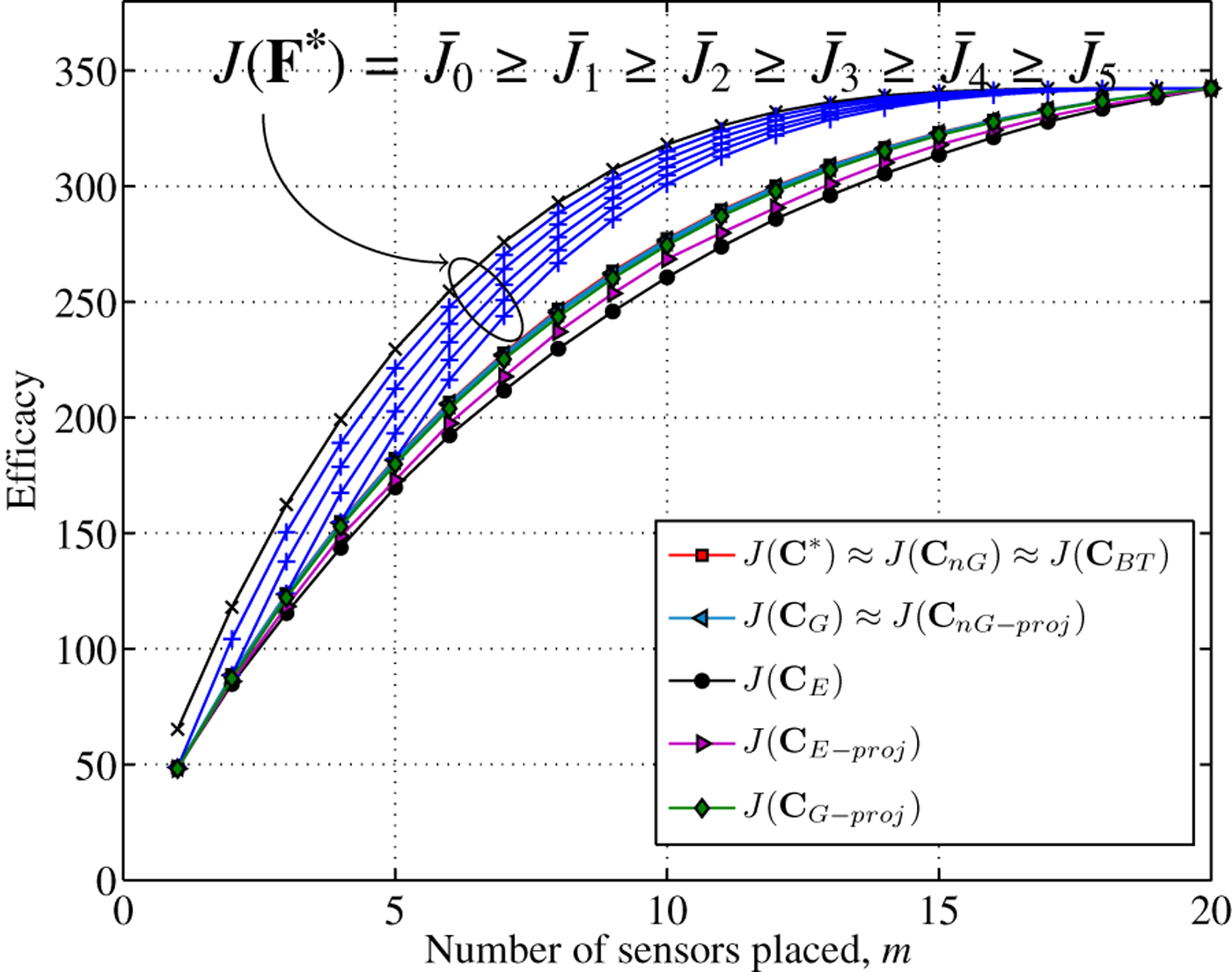
Fig. 1. n = 20: average efficacies of approximate solutions and the upper bound J(F*) compared to the average optimal efficacy J(C*).
We then considered the case for n = 50. For this case, we could not compute the optimal solution because of the prohibitive complexity when n = 50. In Fig. 2, we observe that the projection-based expedient algorithm performs better than the efficacy-based expedient algorithm for some values of m, whereas the latter performs better for other values of m. We also observe that the projection-based n-path greedy algorithm does not always perform better than the efficacy-based greedy algorithm. Therefore, we cannot make an a priori comparison between these algorithms. However, we note that the efficacy-based n-path greedy solution and the backtraced n-path solution perform better than the rest of the algorithms. The upper bound in this case is not tight. Table 1 shows a comparison of average execution time of different proposed algorithms on an Intel Core i3 @ 2.10 GHz machine with 4 GB RAM. From the table, we observe that the projection-based algorithms have similar average runtime as the efficacy-based algorithms.
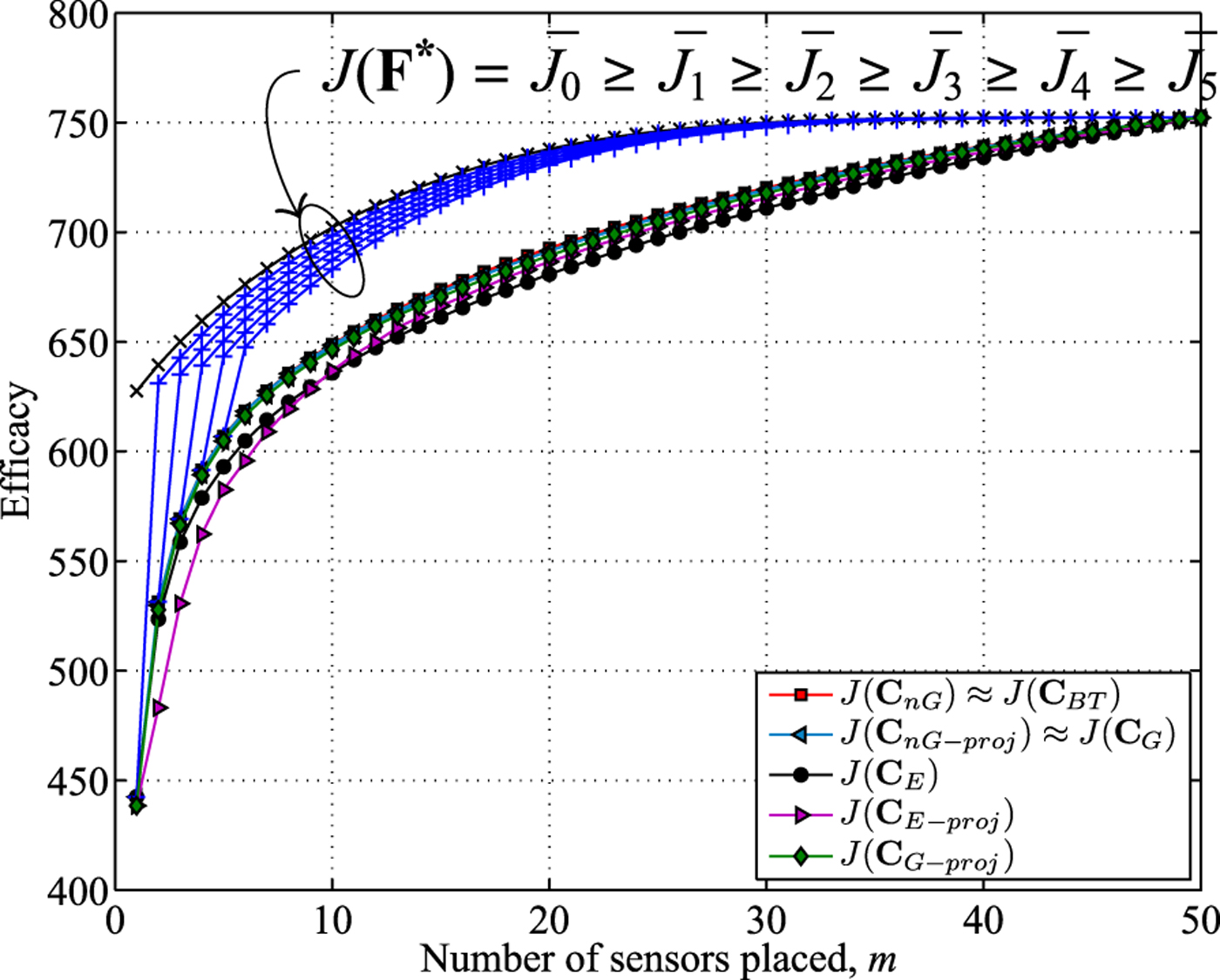
Fig. 2. n = 50: average efficacies of approximate solutions and the upper bound J(F*).
Table 1. Average runtime of proposed algorithms.
B) 5 × 5 grid model
Next, we apply the proposed algorithms to a 5 × 5 grid model where the variance between two points is given in (67). We increased the parameter β from 0.5 to 8.0 in three steps to evaluate the solutions. From Figs. 3–5, we observe that the projection-based expedient solution is not always monotonically increasing. Since the dimension of the upper bounding subspace F* increases as m is increased, the dimension of the subspace closest to F* also increases. As a result the solution subspace for (m + 1) sensors does not always contain the solution subspace for m sensors. Thus, the efficacy obtained by projection-based expedient algorithm is not always monotonic with increasing m.
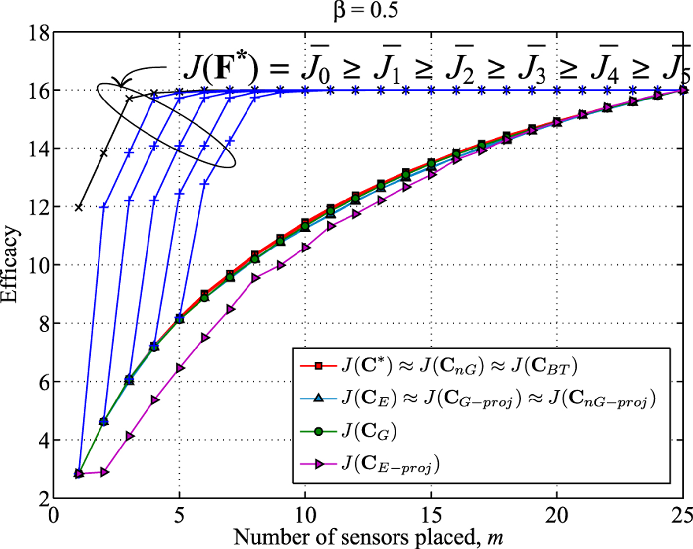
Fig. 3. β = 0.5: efficacies of approximate solutions and the upper bound J(F*) compared to the optimal efficacy J(C*).
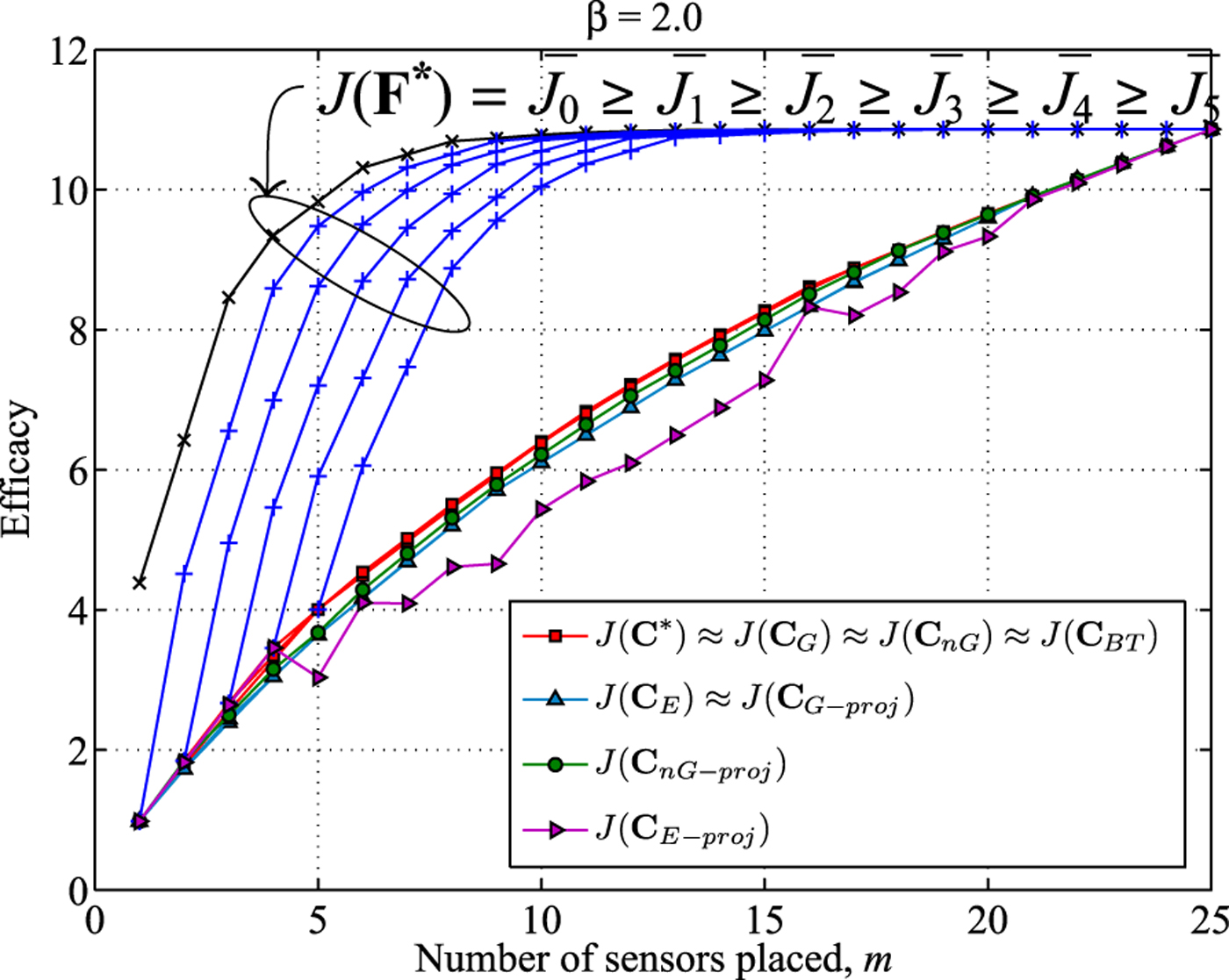
Fig. 4. β = 2.0: efficacies of approximate solutions and the upper bound J(F*) compared to the optimal efficacy J(C*).
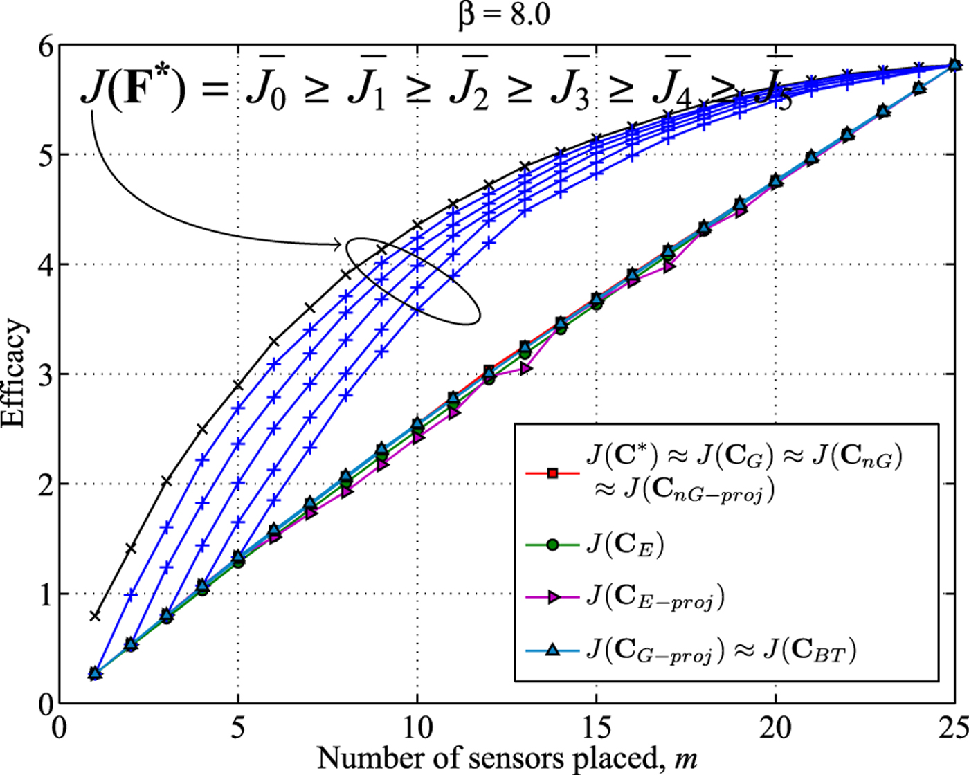
Fig. 5. β = 8.0: Efficacies of approximate solutions and the upper bound J(F*) compared to the optimal efficacy J(C*).
We also note that the projection-based greedy and the n -path greedy algorithm perform better than the efficacy-based expedient solution, but perform worse than the efficacy-based greedy solution in Fig. 3. But the projection-base n -path greedy performs better than efficacy-based greedy solution in Fig. 4, and performs as good as the efficacy-based n -path greedy and backtraced solutions in Fig. 5. The efficacy-based n -path greedy solution and the backtraced n -path solution are almost indistinguishable from the optimal solution in Figs. 3 and 4. In Fig. 5, the backtraced algorithm performs slightly worse than the efficacy-based n-path greedy algorithm. The family of upper bounds from Section IV is not tight in Figs. 3–5. However, the bounds get tighter as β increases.
C) IEEE 57-bus test system
We next apply the proposed sensor placement algorithms to the IEEE 57-bus test system [1]. Traditional state estimators (SE) in the power grid utilize the redundant measurements taken by supervisory control and data acquisition (SCADA) systems, and the states are estimated using iterative algorithms [Reference Abur and Expósito22]. With the advent of phasor technology, time synchronized measurements can be obtained using PMUs. The PMUs can directly measure the states at the PMU-installed buses, and the states of all the connected buses (given enough channels are available) [Reference Phadke and Thorp23]. Thus, the measurement model (1) can be used as the PMU measurement model for the state estimation problem in the power grid. The storage and computational costs of the SE approaches may be further reduced by assuming the voltage magnitudes and phase angles are independent [Reference Huang, Werner, Huang, Kashyap and Gupta24, Reference Monticelli25]. Thus, we consider two independent measurement models for PMU placement, one for voltage magnitudes and the other for phase angles. For simulation purposes, without loss of generality, we assume that the conventional measurements of the test bus system are available to us. We further assume that a sensor is always placed at the swing bus [Reference Phadke and Thorp23] and therefore, the swing bus is not considered in our sensor placement algorithms.
For each measurement model, we construct the sample covariance matrix Σ X by running traditional SE algorithms 1000 times. We used the iterative state estimator based on non-linear AC power flow equations in the MATPOWER software package [Reference Zimmerman, Murillo-Sánchez and Thomas26] for this purpose. Since the measurement noise in the traditional state estimator is Gaussian, the estimated state vectors are also Gaussian [Reference Li, Negi and Ilić9]. In the state estimation process, the standard deviations for voltage magnitudes, bus power injections, and line power flows measurements are 0.01, 0.015, and 0.02, respectively, in accordance with the setups in [Reference Zimmerman, Murillo-Sánchez and Thomas26]. The simulations results of our proposed algorithms and nested bounds for voltage magnitude measurement model and phase angle measurement model are shown in Figs. 6 and 7, respectively. Again due to the size of the system, the exhaustive search for optimal solution was not possible. But it is observed that, for both measurement models, all of the proposed solutions perform very close to each other.
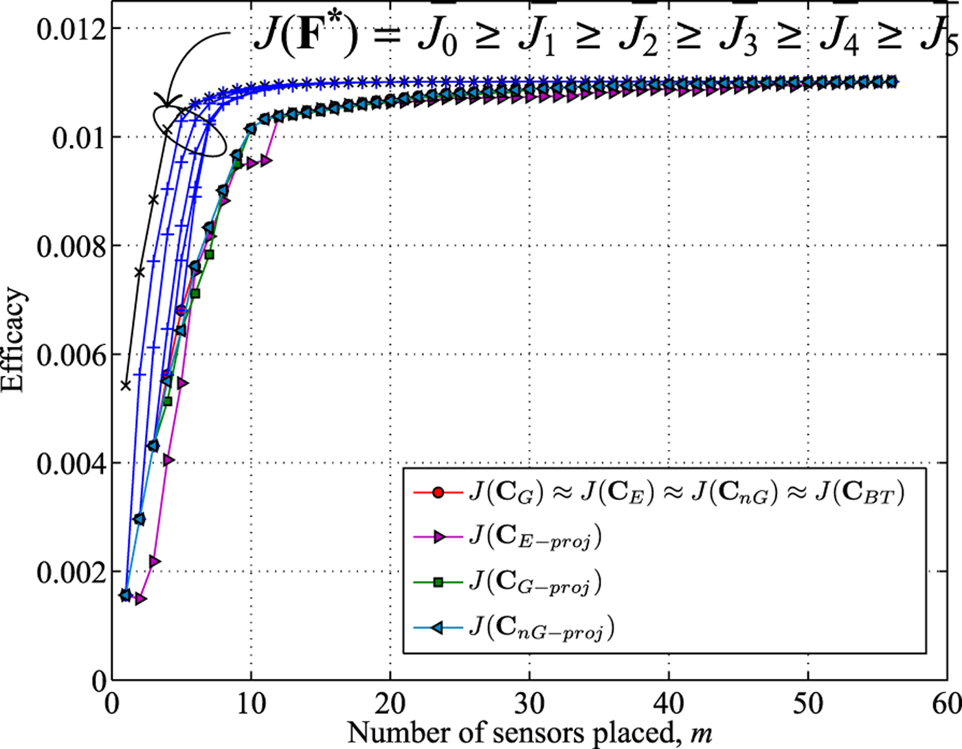
Fig. 6. IEEE 57-bus test case (voltage magnitudes): efficacies of approximate solutions and the upper bound J(F*).
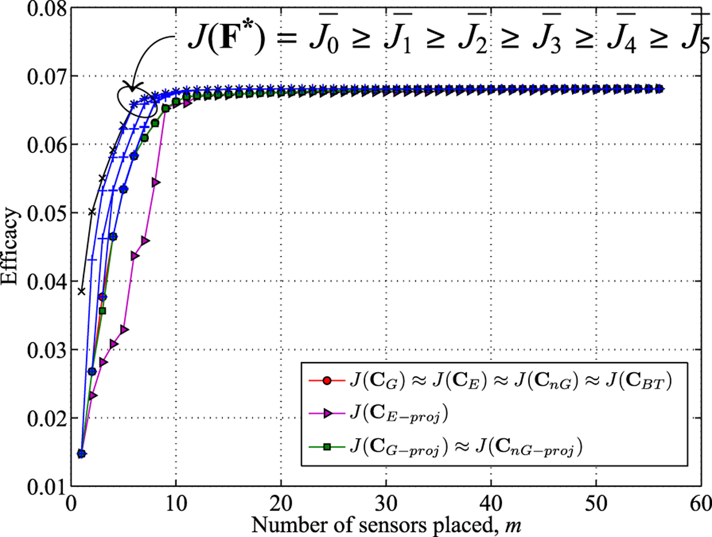
Fig. 7. IEEE 57-bus test case (phase angles): efficacies of approximate solutions and the upper bound J(F*).
VII. SUMMARY AND FURTHER DIRECTIONS
This paper considers the optimal placement of m sensors among n locations. The optimal solution involves solving an integer-programming problem and is NP-complete [Reference Brueni and Heath17]. We came up with a series of approximation algorithms, including a greedy algorithm and a dynamic programming-based algorithm, and their variations that have polynomial complexities. Through simulations we verified that their performances are close to the optimal solution. To further understand the performance of the optimal solution we come up with a series of nested upper bounds (using matrix pencils, generalized eigenvectors, and matrix manipulations) that give tighter upper bounds at increasing complexity. From these nested upper bounds, we found a new set of approximation algorithms that are based on finding projections of unit binary vectors on the subspace generated by the nested upper bounds.
There are many further directions for this research. We would like to come up with tighter upper bounds for the optimal performance. Through simulations we showed that many of the approximation algorithms perform quite well when compared to the optimal algorithm. It would be interesting to come up with tighter theoretical bounds. Algorithms can also be considered when there are additional constraints to the problem (e.g., sensors are not allowed at certain locations), for incremental cases (e.g., want to add some sensors given some sensors have already been placed, which is a generalization of the greedy algorithm), and for dynamic state estimation problems (important for state estimation for the electrical power grid).
In the simulation section, we had an example for an IEEE 57-bus test system. Approximation algorithms perform well and we could apply these algorithms for placement of meters at the distribution level for microgrid state estimation problems. The microgrid has specific local and hierarchical correlations that can be represented by graphs that for the most part are radial. In these cases, perhaps distributed algorithms (such as belief propagation) can be used to find good approximate solutions to the sensor placement problem.
ACKNOWLEDGEMENT
This work was supported in part by the NSF grants ECCS-098344, 1029081, DOE grant DE-OE0000394, and the University of Hawaii REIS project.
APPENDIX A: PROOF OF THEOREM 1
Proof: Using (18), for any
 ${\bf F} \in {\cal F}^{\lsqb m \times n\rsqb }$
, we have
${\bf F} \in {\cal F}^{\lsqb m \times n\rsqb }$
, we have
 $$J_{\left\langle {\bf A}\comma \, {\bf B} \right\rangle} \lpar {\bf F}\rpar = {\rm tr} \left\{\left[{\bf F} {\bf B} {\bf F}^{T} \right]^{-1} {\bf FAF}^{T} \right\}.$$
Let
 $${\bf G} = {\bf FBF}^T.$$
Since G is symmetric positive definite, there exists an m × m invertible matrix G 1/2 such that
 $${\bf G} = {\bf G}^{1/2}{\bf G}^{T/2}.$$
Define M of size m × n as
 $${\bf M} = {\bf G}^{-1/2} {\bf FV}^{-T}.$$
Combining Lemma A with (A.3)–(A.4) we have
 $${\bf MM}^T = {\bf I}_m.$$
Further applying Lemma A and (A.2)–(A.4), the efficacy now reads
 $$J_{\left\langle {\bf A}\comma \, {\bf B} \right\rangle} \lpar {\bf F}\rpar = {\rm tr} \left[{\bf G}^{-1} {\bf F} {\bf A} {\bf F}^{T} \right]$$
 $$= {\rm tr} \left[{\bf G}^{-1} {\bf F} {\bf V}^{-T} {\bf D} {\bf V}^{-1} {\bf F}^{T} \right]$$
 $$= {\rm tr} \left[{\bf G}^{-1} {\bf G}^{1/2} {\bf MDM}^{T} {\bf G}^{T/2} \right]$$
 $$= {\rm tr} \left[{\bf MDM}^{T} \right].$$
Under the constraint (A.5), the efficacy in (A.6) is maximized when M consists of the m eigenvectors of D that correspond to the m highest eigenvalues. Since D is diagonal, eigenvectors of D are the natural basis vectors. Therefore,
 $${\bf M}^{\ast} = \left[\matrix{{\bf I}_m & {\bf 0}} \right].$$
Thus, by substituting (A.10) into (A.6), the optimal efficacy J 〈A, B〉* becomes
 $$J_{\left\langle {\bf A}\comma \, {\bf B}\right\rangle}^{\ast} = {\rm tr} \left\{\left[\matrix{{\bf I}_m &{\bf 0}} \right]{\bf D} \left[\matrix{{\bf I}_m & {\bf 0}} \right]^T \right\}= \sum_{j = 1}^{m} \delta_j.$$
Now set
 ${\bf F} = {\bf M}^{\ast}{\bf V}^T = \left[\matrix{{\bf I}_m & {\bf 0}} \right]{\bf V}^T$
, and verify (using Lemma A) that this choice of F has efficacy J
〈A, B〉 (F) that equals to the maximal efficacy in (A.11). Consequently, the optimal argument must equal
${\bf F} = {\bf M}^{\ast}{\bf V}^T = \left[\matrix{{\bf I}_m & {\bf 0}} \right]{\bf V}^T$
, and verify (using Lemma A) that this choice of F has efficacy J
〈A, B〉 (F) that equals to the maximal efficacy in (A.11). Consequently, the optimal argument must equal
 $${\bf F}^{\ast}_{\left\langle {\bf A}\comma \, {\bf B} \right\rangle} = \left[\matrix{{\bf I}_m & {\bf 0}} \right]{\bf V}^T = \left[\matrix{\underline{v}_1 & \cdots & \underline{v}_m} \right]^T.$$
□
APPENDIX B: PROOF OF LEMMA B
Proof: For any
 ${\bf F} \in {\cal F}^{\lsqb \lpar m-k\rpar \times \lpar n-k\rpar \rsqb }$
, using (18) we express the efficacy as
${\bf F} \in {\cal F}^{\lsqb \lpar m-k\rpar \times \lpar n-k\rpar \rsqb }$
, using (18) we express the efficacy as
 $$\eqalign{J_{\left\langle {\bf A}\comma \, {\bf B} \right\rangle} \left(\left[\matrix{{\bf I}_k & {\bf 0}\cr {\bf 0} & {\bf F}} \right]\right)&= {\rm tr} \left\{\left(\left[\matrix{{\bf I}_k &{\bf 0}\cr {\bf 0} &{\bf F}} \right]{\bf B} \left[\matrix{{\bf I}_k&{\bf 0}\cr {\bf 0}&{\bf F}} \right]^{T}\right)^{-1} \right. \cr &\left. \quad \times \left[\matrix{{\bf I}_k&{\bf 0}\cr {\bf 0}&{\bf F}} \right]{\bf A} \left[\matrix{{\bf I}_k&{\bf 0}\cr {\bf 0}&{\bf F}} \right]^{T} \right\}.}$$
Using (37), (38), and (39), we express B in terms of P k , Q k and R k as
 $${\bf B} = \left[\matrix{{\bf P}_k & {\bf Q}_k \cr {\bf Q}_k^T & {\bf R}_k} \right].$$
Substituting B into (B.1) and using the partitioned matrix inversion lemma [Reference Abadir and Magnus27], we write (B.1) as
 $$\eqalign{&J_{\left\langle {\bf A}\comma \, {\bf B} \right\rangle} \left(\left[\matrix{ {\bf I}_k & {\bf 0}\cr {\bf 0} & {\bf F}} \right]\right)\cr &\quad = {\rm tr}\left\{{\bf A} \left[\matrix{ {\bf P}_k^{-1} & {\bf 0} \cr {\bf 0} & {\bf 0}} \right]\right\}+ {\rm tr} \left\{\left[\matrix{{\bf P}_k^{-1}{\bf Q}_k{\bf F}^{T} \cr -{\bf I}_{m-k}} \right]\right. \cr &\left. \qquad \times \left\{{\bf F} \left({\bf R}_k\, {-}\, {\bf Q}^{T}{\bf P}_k^{-1}{\bf Q}_k\right){\bf F}^{T}\right\}^{-1} \left[\matrix{{\bf P}_k^{-1}{\bf Q}_k{\bf F}^{T} \cr -{\bf I}_{m-k}} \right]^{T} \right. \cr &\left. \qquad \times \left[\matrix{ {\bf I}_k&{\bf 0}\cr {\bf 0}&{\bf F}} \right]{\bf A} \left[\matrix{ {\bf I}_k&{\bf 0}\cr {\bf 0}&{\bf F}} \right]^{T} \right\}.}$$
Using (34), (35), and (36), we simplify (B.3) as
 $$J_{\left\langle {\bf A}\comma {\bf B} \right\rangle} \left(\left[\matrix{ {\bf I}_k & {\bf 0}\cr {\bf 0} & {\bf F}} \right]\right)= t_k\, {+}\, {\rm tr} \left\{\left({\bf F} {\bf B}_k {\bf F}^T \right)^{-1} {\bf F} {\bf A}_k {\bf F}^T \right\}$$
 $$= t_k\, {+}\, J_{\left\langle {\bf A}_k\comma \, {\bf B}_k \right\rangle} \lpar {\bf F}\rpar.$$
Muhammad Sharif Uddin received his B.Sc. degree in Electrical and Electronic Engineering from Bangladesh University of Engineering and Technology, Dhaka, Bangladesh, in 2009. He is currently pursuing the Ph.D. degree in Electrical Engineering at the University of Hawaii at Manoa. His research interests include sensor networks, signal processing, machine learning, and smart grid applications.
Anthony Kuh received his B.S. degree in Electrical Engineering and Computer Science at the University of California, Berkeley in 1979, an M.S. degree in Electrical Engineering from Stanford University in 1980, and a Ph.D. degree in Electrical Engineering from Princeton University in 1987. Dr. Kuh previously worked at AT&T Bell Laboratories and has been on the faculty in Electrical Engineering at the University of Hawaii since 1986. He is currently a Professor in the Department and is also currently serving as the director of the Interdisciplinary Renewable Energy and Island Sustainability (REIS) Group. Previously, he served as the Department Chair of Electrical Engineering. Dr. Kuh's research is in the area of neural networks and machine learning, adaptive signal processing, sensor networks, communication networks, and renewable energy and smart grid applications. Dr. Kuh won a National Science Foundation Presidential Young Investigator Award, received a Distinguished Fulbright Scholar's Award working at Imperial College, London, and is an IEEE Fellow. He is currently serving as the IEEE Signal Processing Society Regions 1-6 Director at Large, on the Board of Governors of the Asia Pacific Signal and Information Processing Association, and as a senior editor of the IEEE Journal of Selected Topics in Signal Processing.
Aleksandar Kavcic received the Dipl. Ing. degree in Electrical Engineering from Ruhr-University, Bochum, Germany in 1993, and the Ph.D. degree in Electrical and Computer Engineering from Carnegie Mellon University in 1998. Currently, he is a Professor of Electrical Engineering at the University of Hawaii. Professor Kavcic received the IBM Partnership Award in 1999 and NSF CAREER Award in 2000. He is a co-recipient of the 2005 IEEE Best Paper Award in Signal Processing and Coding for Data Storage. He served as Associate Editor of the IEEE Transactions on Information Theory from 2001 to 2004, as Guest Editor of the IEEE Signal Processing Magazine in 2003–2004, and as Guest Editor of the IEEE Journal on Selected Areas in Communications in 2008–2009. From 2005 until 2007, he was the Chair of the DSTC of the IEEE Communications Society, and in 2014 was the general co-chair of the IEEE ISIT in Honolulu, Hawaii.
Toshihisa Tanaka received the B.E., M.E., and Ph.D. degrees from Tokyo Institute of Technology in 1997, 2000, and 2002, respectively. He joined the Department of Electrical and Electronic Engineering, Tokyo University of Agriculture and Technology, in 2004, where he is currently an Associate Professor. In 2005, he was a Royal Society Visiting Fellow at Imperial College London, UK. In 2011, he was a Visiting Faculty Member at University of Hawaii. He is a coeditor of Signal Processing Techniques for Knowledge Extraction and Information Fusion (Springer 2008). His research interests include image and signal processing, statistical signal processing and machine learning, biomedical signal processing, and adaptive systems.
Dr. Tanaka has served on the editorial board for several major international journals. He is a Past-Chair of the TC on Biomedical Signal Processing, APSIPA. He is a senior member of the IEEE, and a member of the IEICE and APSIPA.


 Open access