


Impact Statement
The use of graph neural networks wall models for compressible anisothermal flows has the potential to significantly enhance the accuracy and efficiency of large-eddy simulation in industrial settings. This innovation can lead to improvements in design optimization in various industries, notably in the transportation, aeronautics, and energy sectors, and thus contribute to global sustainability goals by helping to decarbonize these sectors.
1. Introduction
It is often computationally impractical to simulate all scales of motions in turbulent fluid flows. The computational requirements are less stringent if only the larger turbulent scales are resolved, and the smaller ones modeled. This is the basis of large-eddy simulation (LES). By modeling the effect of the more expensive small-scale motions, LESs enable the study of more complex flow configurations than allowed by direct computation. The LES of compressible anisothermal flow, in particular, is useful in many industrial applications, such as combustion chambers, high-pressure turbines, rocket engines, or heat exchangers (Chassaing et al., Reference Chassaing, Antonia, Anselmet, Joly and Sarkar2013). In these flows, the variations of density, viscosity, or heat conductivity with temperature are large and lead to a strong coupling between the fields of temperature and velocity. The near-wall profiles of velocity and temperature are influenced by this coupling (Huang et al., Reference Huang, Coleman and Bradshaw1995; Serra et al., Reference Serra, Toutant, Bataille and Zhou2012; Toutant and Bataille, Reference Toutant and Bataille2013). LES should thus accurately represent the interaction between temperature and turbulence. There are two ways to approach the simulation of wall-bounded compressible anisothermal flow. The first approach, hereafter referred to as wall-resolved large-eddy simulation (WRLES), resolves the large-scale turbulent structures in the entire boundary layer, including the viscous and conductive sublayers. Since the turbulent structures decrease in size near walls, this can be costly at high Reynolds numbers and for complex configurations. The second approach, hereafter referred to as wall-modeled large-eddy simulation (WMLES), models all turbulent structures in the viscous and conductive sublayers. This can be achieved using a wall model that imposes either the shear stress, conductive heat flux, slip velocity, or temperature at the wall as a boundary condition.
Various wall models have been proposed in the literature. Differential wall models can be devised by combining large-eddy simulation with Reynolds-average Navier–Stokes (RANS) near the walls. Hybrid methods based on an embedded grid, zonal methods, and seamless methods such as detached-eddy simulation may fall into this category (Cabot, Reference Cabot1995; Balaras et al., Reference Balaras, Benocci and Piomelli1996; Davidson and Peng, Reference Davidson and Peng2003; Temmerman et al., Reference Temmerman, Hadžiabdić, Leschziner and Hanjalić2005; Piomelli, Reference Piomelli2008). This type of approach can handle non-equilibrium effects (Kawai and Larsson, Reference Kawai and Larsson2013; Park and Moin, Reference Park and Moin2014) and may take into account the effects of compressibility and temperature variations, provided that relevant RANS models are used (Benarafa et al., Reference Benarafa, Cioni, Ducros and Sagaut2007; Rani et al., Reference Rani, Smith and Nix2009; Zhang et al., Reference Zhang, Vicquelin, Gicquel and Taine2013; Mettu and Subbareddy, Reference Mettu and Subbareddy2018; Iyer and Malik, Reference Iyer and Malik2019). However, the computational cost can be large as it requires a mesh that resolves the viscous and conductive sublayers for the RANS computation. To reduce computational costs, an integral wall model based on a parameterized velocity profile was introduced by Yang et al. (Reference Yang, Sadique, Mittal and Meneveau2015) for incompressible flows and extended to compressible anisothermal flows by Catchirayer et al. (Reference Catchirayer, Boussuge, Sagaut, Montagnac, Papadogiannis and Garnaud2018). The family of algebraic wall models includes some of the most widely used and classical wall models (Larsson et al., Reference Larsson, Kawai, Bodart and Bermejo-Moreno2016; Bose and Park, Reference Bose and Park2018). The simplest such model uses the incompressible law of the wall locally and instantaneously, following a statistical equilibrium assumption, to impose the wall shear stress (Deardorff, Reference Deardorff1970; Schumann, Reference Schumann1975). The approach may be adapted to the modeling of the conductive heat flux using a wall function for temperature (Kader and Yaglom, Reference Kader and Yaglom1972; Han and Reitz, Reference Han and Reitz1997; Nichols and Nelson, Reference Nichols and Nelson2004; Berni et al., Reference Berni, Cicalese and Fontanesi2017). The law of the wall for temperature fields has been analyzed by Huang et al. (Reference Huang, Coleman and Bradshaw1995). The article also introduced the semi-local scaling analysis, which is relevant for wall modeling (Patel et al., Reference Patel, Peeters, Boersma and Pecnik2015, Reference Patel, Boersma and Pecnik2016, Reference Patel, Boersma and Pecnik2017). The models for velocity and temperature should necessarily be coupled in flows with strong temperature variations, as for example was proposed by Cabrit and Nicoud (Reference Cabrit and Nicoud2009). This coupled wall model has been validated and compared to uncoupled wall modeling approaches and differential wall models in various physical configurations (Maestro et al., Reference Maestro, Cuenot and Selle2017; Kraus et al., Reference Kraus, Selle and Poinsot2018; Muto et al., Reference Muto, Daimon, Shimizu and Negishi2019, Reference Muto, Daimon, Negishi and Shimizu2021; Indelicato et al., Reference Indelicato, Lapenna, Remiddi and Creta2021; Potier et al., Reference Potier, Duchaine, Cuenot, Saucereau and Pichillou2022). Finally, machine-learning wall models have recently emerged following the development of machine-learning technologies in image classification, speech recognition, natural language processing as well as turbulence simulation and modeling (LeCun et al., Reference LeCun, Bengio and Hinton2015; Duraisamy et al., Reference Duraisamy, Iaccarino and Xiao2019; Brunton et al., Reference Brunton, Noack and Koumoutsakos2020). Data-driven wall-stress models were developed and assessed for various incompressible flow configurations, including fully developed wall turbulence and separated turbulent flows (Huang et al., Reference Huang, Yang and Kunz2019; Yang et al., Reference Yang, Zafar, Wang and Xiao2019; Lozano-Durán and Bae, Reference Lozano-Durán and Bae2020, Reference Lozano-Durán and Bae2022; Bhaskaran et al., Reference Bhaskaran, Kannan, Barr and Priebe2021; Radhakrishnan et al., Reference Radhakrishnan, Adu, Miró, Font, Calafell and Lehmkuhl2021; Zangeneh, Reference Zangeneh2021; Zhou et al., Reference Zhou, He and Yang2021; Bae and Koumoutsakos, Reference Bae and Koumoutsakos2022; Dupuy et al., Reference Dupuy, Odier and Lapeyre2023a). For complex configurations, Dupuy et al. (Reference Dupuy, Odier, Lapeyre and Papadogiannis2023b) introduced a machine-learning wall model that can directly operate on the unstructured grid of a LES, based on a graph neural network (GNN) architecture (Battaglia et al., Reference Battaglia, Hamrick, Bapst, Sanchez-Gonzalez, Zambaldi, Malinowski, Tacchetti, Raposo, Santoro, Faulkner, Gulcehre, Song, Ballard, Gilmer, Dahl, Vaswani, Allen, Nash, Langston, Dyer, Heess, Wierstra, Kohli, Botvinick, Vinyals, Li and Pascanu2018; Pfaff et al., Reference Pfaff, Fortunato, Sanchez-Gonzalez and Battaglia2020; Zhou et al., Reference Zhou, Cui, Hu, Zhang, Yang, Liu, Wang, Li and Sun2020). The relevance of the approach was demonstrated a priori and a posteriori for the modeling of the wall shear stress in incompressible isothermal flows.
In this article, the GNN wall modeling approach is extended to the modeling of the wall shear stress and wall conductive heat flux in compressible anisothermal flows. The objective is to assess the capability of graph neural network to address the wall modeling of complex anisothermal flows, as well as to evaluate the generalization capabilities of such models. The graph neural networks are based on an Encode-Process-Decode architecture (Battaglia et al., Reference Battaglia, Hamrick, Bapst, Sanchez-Gonzalez, Zambaldi, Malinowski, Tacchetti, Raposo, Santoro, Faulkner, Gulcehre, Song, Ballard, Gilmer, Dahl, Vaswani, Allen, Nash, Langston, Dyer, Heess, Wierstra, Kohli, Botvinick, Vinyals, Li and Pascanu2018) with no global features that ensure the spatial locality of the prediction. Due to the GNN architecture, the model is able to directly operate on unstructured meshes and can be applied in complex geometries with angles or curvature without a prior interpolation of the inputs. Moreover, the GNN architecture encodes the translational invariance of the prediction, is inherently biased toward locality and suited to massively parallel computation. The inputs of the model are augmented and scaled to ensure in addition the Galilean invariance of the model and the equivariance of the model under orthogonal transformations and to Mach number variations. Although the GNN approach is in principle not restrictive in terms of mesh elements, the present analysis is restricted to coarse tetrahedral meshes, as this type of mesh is commonly used to simulate complex industrial flows. The graph neural networks wall models are validated a priori, based on filtered numerical data from direct numerical simulations (DNS) and wall-resolved LESs, and a posteriori, based on wall-modeled LESs coupled with the GNN models. The models are trained and tested on coarse tetrahedral meshes in both cases. We use an uncoupled velocity-temperature algebraic wall model and the coupled velocity-temperature algebraic wall model of Cabrit and Nicoud (Reference Cabrit and Nicoud2009) as baseline wall models in both cases. The a priori database used to train and evaluate the models include six incompressible isothermal flows (two channel flows, a diffuser, two backward-facing steps, and a linear blade cascade) and five compressible anisothermal flows (two symmetrically cooled channel flows, two asymmetrically cooled/heated channels flows, and a cooled high-pressure turbine blade). In a posteriori tests, the model is first assessed for a channel flow to verify that the graph neural network model is able to perform at least as well as algebraic models devised for this type of simulation. The model is then validated a posteriori for the simulation of the high-pressure turbine blade VKI LS1989, specifically for test case MUR235 of Arts et al. (Reference Arts, Rouvroit and Rutherford1990), which features a complex physics that strongly departs from equilibrium wall modeling assumptions. It relies on the coupling strategy of Serhani et al. (Reference Serhani, Xing, Dupuy, Lapeyre and Staffelbach2022) to couple the massively parallel flow solver (Schönfeld and Rudgyard, Reference Schönfeld and Rudgyard1999) to the graph neural network in the wall-modeled LESs.
The article is organized as follows. The dataset and the preparation of the data for the machine-learning model are presented in Section 2. The strategies used to enforce the equivariances of the model are described in Section 3. The baseline wall models and the graph neural network wall model are described in Section 4. The a priori results are discussed in Section 5 and the a posteriori results in Section 6.
2. Database
Data-driven wall modeling hinges on the development of datasets that can specify the wall behavior of fluids. These datasets may either be based on high-fidelity experimental or numerical data, and should involve a large diversity of flow phenomena in order to build a model that can operate in a wide variety of configurations. Building such dataset is a challenging task, even if the problem is restricted to incompressible flows. The effect of compressibility and fluid-property variations adds several dimensions to the problem, for instance, the effect of the Prandtl number, the Mach number, the equation of state, or the viscosity law, such that fully specifying the problem is yet elusive. For practical purpose, small regions of the problem space, of practical interest, could however be described by such a dataset. The present study uses a dataset of 12 high-fidelity numerical simulations, 6 incompressible isothermal simulations, and 5 compressible anisothermal simulations. All compressible simulations involve an ideal gas, with properties close to that of air in terms of Prandtl number, assumed constant. The simulations were performed by various research groups using various CFD solvers and numerical methods. Demonstrating an ability to learn from such an heterogeneous database is crucial for the further development of machine-learning wall models with much larger datasets. The six incompressible isothermal simulations are the same as found in Dupuy et al. (Reference Dupuy, Odier, Lapeyre and Papadogiannis2023b), as summarized in Table 1: two fully developed channel flows at friction Reynolds number
 $ {\mathit{\operatorname{Re}}}_{\tau }=180 $
(CF1, (Agostini and Vincent, Reference Agostini and Vincent2020) and
$ {\mathit{\operatorname{Re}}}_{\tau }=180 $
(CF1, (Agostini and Vincent, Reference Agostini and Vincent2020) and
 $ {\mathit{\operatorname{Re}}}_{\tau }=950 $
(CF2, (Del Álamo and Jiménez, Reference Del Álamo and Jiménez2003; Lozano-Durán and Jiménez, Reference Lozano-Durán and Jiménez2014; Lozano-Durán and Jiménez, Reference Lozano-Durán and Jiménez2015); a three-dimensional diffuser corresponding to the geometry “Diffuser 1” of Cherry et al. (Reference Cherry, Elkins and Eaton2008) (3DD, (Ercoftac, 2022); a backward-facing step (BFS, (Pouech et al., Reference Pouech, Duchaine and Poinsot2019, Reference Pouech, Duchaine and Poinsot2021); a curved backward-facing step (APG, (Ercoftac, 2022); and a NACA 65–009 blade cascade on a flat plate such as studied experimentally by Ma et al. (Reference Ma, Ottavy, Lu, Francis and Gao2011) and Zambonini et al. (Reference Zambonini, Ottavy and Kriegseis2017) at an incidence angle of 4° and 7° (N65) (Dupuy et al., Reference Dupuy, Odier, Lapeyre and Papadogiannis2023b). The five compressible anisothermal simulations are the simulations of two fully developed asymmetrically cooled/heated channel flows at friction Reynolds number
$ {\mathit{\operatorname{Re}}}_{\tau }=950 $
(CF2, (Del Álamo and Jiménez, Reference Del Álamo and Jiménez2003; Lozano-Durán and Jiménez, Reference Lozano-Durán and Jiménez2014; Lozano-Durán and Jiménez, Reference Lozano-Durán and Jiménez2015); a three-dimensional diffuser corresponding to the geometry “Diffuser 1” of Cherry et al. (Reference Cherry, Elkins and Eaton2008) (3DD, (Ercoftac, 2022); a backward-facing step (BFS, (Pouech et al., Reference Pouech, Duchaine and Poinsot2019, Reference Pouech, Duchaine and Poinsot2021); a curved backward-facing step (APG, (Ercoftac, 2022); and a NACA 65–009 blade cascade on a flat plate such as studied experimentally by Ma et al. (Reference Ma, Ottavy, Lu, Francis and Gao2011) and Zambonini et al. (Reference Zambonini, Ottavy and Kriegseis2017) at an incidence angle of 4° and 7° (N65) (Dupuy et al., Reference Dupuy, Odier, Lapeyre and Papadogiannis2023b). The five compressible anisothermal simulations are the simulations of two fully developed asymmetrically cooled/heated channel flows at friction Reynolds number
 $ {\mathit{\operatorname{Re}}}_{\tau }=180 $
(AC1, (Dupuy et al., Reference Dupuy, Toutant and Bataille2018) and
$ {\mathit{\operatorname{Re}}}_{\tau }=180 $
(AC1, (Dupuy et al., Reference Dupuy, Toutant and Bataille2018) and
 $ {\mathit{\operatorname{Re}}}_{\tau }=395 $
(AC2, (Dupuy et al., Reference Dupuy, Toutant and Bataille2019), with a temperature ratio of 2 between the two walls; two fully developed symmetrically cooled channel flows at friction Reynolds number
$ {\mathit{\operatorname{Re}}}_{\tau }=395 $
(AC2, (Dupuy et al., Reference Dupuy, Toutant and Bataille2019), with a temperature ratio of 2 between the two walls; two fully developed symmetrically cooled channel flows at friction Reynolds number
 $ {\mathit{\operatorname{Re}}}_{\tau }=320 $
(SC1, Appendix A) and
$ {\mathit{\operatorname{Re}}}_{\tau }=320 $
(SC1, Appendix A) and
 $ {\mathit{\operatorname{Re}}}_{\tau }=1150 $
(SC2, Appendix A), with a temperature ratio between the bulk flow and the walls of 1.1 and 3 respectively; and a cooled high-pressure turbine blade which corresponds to the test case MUR235 of Arts et al. (Reference Arts, Rouvroit and Rutherford1990) (L89, (Dupuy et al., Reference Dupuy, Gicquel, Odier, Duchaine and Arts2020). The SC1 simulation aims to provide a case where the coupling between the velocity and temperature fields is small, while the SC2, AC1, and AC2 simulations provide cases where this coupling is strong. The channel flows simulations (CF1, CF2, AC1, AC2, SC1, SC2) provide data for fully developed attached turbulence, whereas the spatially inhomogeneous simulations (3DD, BFS, APG, N65, L89) provide data in non-equilibrium conditions, including regions with adverse pressure gradients, separated boundary layers, and laminar-turbulent transition. The N65 and L89 simulations feature laminar and transitional boundary layers on the blade surface. The 3DD simulation includes an intermittently laminar-separated region (Ohlsson et al., Reference Ohlsson, Schlatter, Fischer and Henningson2010). The numerical parameters of each simulation are summarized in Table 1.
$ {\mathit{\operatorname{Re}}}_{\tau }=1150 $
(SC2, Appendix A), with a temperature ratio between the bulk flow and the walls of 1.1 and 3 respectively; and a cooled high-pressure turbine blade which corresponds to the test case MUR235 of Arts et al. (Reference Arts, Rouvroit and Rutherford1990) (L89, (Dupuy et al., Reference Dupuy, Gicquel, Odier, Duchaine and Arts2020). The SC1 simulation aims to provide a case where the coupling between the velocity and temperature fields is small, while the SC2, AC1, and AC2 simulations provide cases where this coupling is strong. The channel flows simulations (CF1, CF2, AC1, AC2, SC1, SC2) provide data for fully developed attached turbulence, whereas the spatially inhomogeneous simulations (3DD, BFS, APG, N65, L89) provide data in non-equilibrium conditions, including regions with adverse pressure gradients, separated boundary layers, and laminar-turbulent transition. The N65 and L89 simulations feature laminar and transitional boundary layers on the blade surface. The 3DD simulation includes an intermittently laminar-separated region (Ohlsson et al., Reference Ohlsson, Schlatter, Fischer and Henningson2010). The numerical parameters of each simulation are summarized in Table 1.
Table 1. Numerical parameters of the numerical simulations are included in the training database
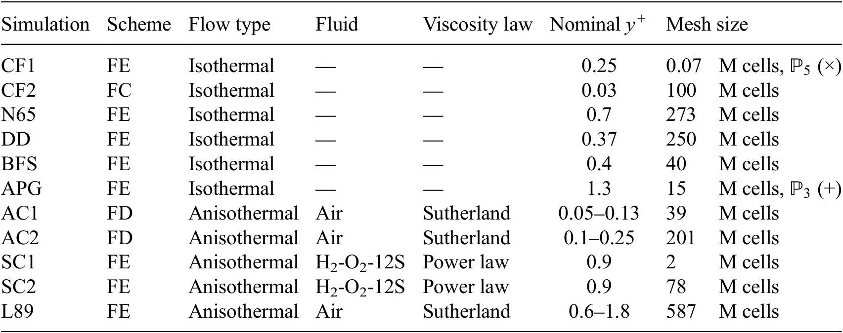
Note. The acronym FC denotes a Fourier-Chebyshev spectral method, FE denotes a finite-element method and FD denotes a finite-difference method.
 $ {\mathrm{\mathbb{P}}}_n $
indicates the use of a high-order method with polynomial order
$ {\mathrm{\mathbb{P}}}_n $
indicates the use of a high-order method with polynomial order
 $ n $
. The “nominal
$ n $
. The “nominal
 $ {y}^{+} $
” is the height of the first point off the wall, in wall units, in the channel (CF1, CF2, SC1, SC2), the boundary layer upstream of the blade (N65), the inlet duct flow (3DD), the boundary layer before the step (BFS, APG), the bottom (cold) and top (hot) walls (AC1, AC2), the blade surface on the pressure and suction sides (L89). An “isothermal” flow type implies that the temperature variations within the flow are negligible but does not imply an incompressible numerical method. In the case where a compressible numerical solver is used to simulate an incompressible isothermal flow, we do not report the fluid and viscosity law since it is not of practical relevance.
$ {y}^{+} $
” is the height of the first point off the wall, in wall units, in the channel (CF1, CF2, SC1, SC2), the boundary layer upstream of the blade (N65), the inlet duct flow (3DD), the boundary layer before the step (BFS, APG), the bottom (cold) and top (hot) walls (AC1, AC2), the blade surface on the pressure and suction sides (L89). An “isothermal” flow type implies that the temperature variations within the flow are negligible but does not imply an incompressible numerical method. In the case where a compressible numerical solver is used to simulate an incompressible isothermal flow, we do not report the fluid and viscosity law since it is not of practical relevance.
2.1. Data preparation
The fields in the numerical database are processed to prepare the data for the machine-learning wall models. The goal of this preprocessing step is to produce fields that are similar in some ways to the fields of a wall-modeled LES. Namely, the fields are filtered to attenuate large frequencies that cannot be resolved in a wall-modeled LES and resampled onto coarse tetrahedral meshes that could be used for WMLES computations. The present machine-learning methodology does not make any assumption regarding the nature of the function that should be learned by the model and can only operate in the range of mesh resolution that was seen during training. This operating range effectively determines the range of Reynolds number that can be addressed a posteriori at moderate computational cost. Since the exact mesh resolution required for unseen test cases is not known, it is important to consider a wide range of mesh refinements to train the model. For each simulation, 12 tetrahedral WMLES meshes with varying mesh resolution are generated using the mesh adaptation library MMG3D (Dobrzynski and Frey, Reference Dobrzynski and Frey2008; Dapogny et al., Reference Dapogny, Dobrzynski and Frey2014; Balarac et al., Reference Balarac, Basile, Bénard, Bordeu, Chapelier, Cirrottola, Caumon, Dapogny, Frey, Froehly, Ghigliotti, Laraufie, Lartigue, Legentil, Mercier, Moureau, Nardoni, Pertant and Zakari2021), with nominal edge length in the range
 $ 25\le {e}^{+}\le 80 $
, in wall units, where the classical wall-unit scaling is based on the friction velocity and the kinematic viscosity at the wall, namely
$ 25\le {e}^{+}\le 80 $
, in wall units, where the classical wall-unit scaling is based on the friction velocity and the kinematic viscosity at the wall, namely
 $ {e}^{+}={eu}_{\tau }/{\nu}_{\omega } $
, with
$ {e}^{+}={eu}_{\tau }/{\nu}_{\omega } $
, with
 $ e $
the nominal edge length,
$ e $
the nominal edge length,
 $ {u}_{\tau }={\left(\tau /{\rho}_{\omega}\right)}^{0.5} $
the friction velocity,
$ {u}_{\tau }={\left(\tau /{\rho}_{\omega}\right)}^{0.5} $
the friction velocity,
 $ \tau $
the wall shear stress,
$ \tau $
the wall shear stress,
 $ {\rho}_{\omega } $
the wall density, and
$ {\rho}_{\omega } $
the wall density, and
 $ {\nu}_{\omega } $
the wall kinematic viscosity. This range of
$ {\nu}_{\omega } $
the wall kinematic viscosity. This range of
 $ {e}^{+} $
implies that the first point off the wall of the WMLES mesh is typically within the logarithmic layer or the upper part of the buffer layer, in the case of a fully developed turbulent boundary layer. It is suitable for instance in turbomachinery-flow simulations (Leonard et al., Reference Leonard, Sanjose, Moreau and Duchaine2016; Dombard et al., Reference Dombard, Duchaine, Gicquel, Odier, Leroy, Buffaz, Le-Guyader, Démolis, Richard and Grosnickel2020; Odier et al., Reference Odier, Thacker, Harnieh, Staffelbach, Gicquel, Duchaine, Rosa and Müller2021). Indeed, while real turbomachines are typically not instrumented for boundary-layer measurements, experimental measurements, and high-fidelity LESs show that the friction Reynolds number based on boundary-layer thickness is in the range of 600–1000 in academic linear blade cascades with realistic operating conditions in terms of Reynolds and Mach numbers (Arts et al., Reference Arts, Rouvroit and Rutherford1990; Ma et al., Reference Ma, Ottavy, Lu, Francis and Gao2011; Gao et al., Reference Gao, Zambonini, Boudet, Ottavy, Lu and Shao2015; Zambonini et al., Reference Zambonini, Ottavy and Kriegseis2017; Dupuy et al., Reference Dupuy, Gicquel, Odier, Duchaine and Arts2020). However, this implies that the trained models are not applicable for cell sizes larger than
$ {e}^{+} $
implies that the first point off the wall of the WMLES mesh is typically within the logarithmic layer or the upper part of the buffer layer, in the case of a fully developed turbulent boundary layer. It is suitable for instance in turbomachinery-flow simulations (Leonard et al., Reference Leonard, Sanjose, Moreau and Duchaine2016; Dombard et al., Reference Dombard, Duchaine, Gicquel, Odier, Leroy, Buffaz, Le-Guyader, Démolis, Richard and Grosnickel2020; Odier et al., Reference Odier, Thacker, Harnieh, Staffelbach, Gicquel, Duchaine, Rosa and Müller2021). Indeed, while real turbomachines are typically not instrumented for boundary-layer measurements, experimental measurements, and high-fidelity LESs show that the friction Reynolds number based on boundary-layer thickness is in the range of 600–1000 in academic linear blade cascades with realistic operating conditions in terms of Reynolds and Mach numbers (Arts et al., Reference Arts, Rouvroit and Rutherford1990; Ma et al., Reference Ma, Ottavy, Lu, Francis and Gao2011; Gao et al., Reference Gao, Zambonini, Boudet, Ottavy, Lu and Shao2015; Zambonini et al., Reference Zambonini, Ottavy and Kriegseis2017; Dupuy et al., Reference Dupuy, Gicquel, Odier, Duchaine and Arts2020). However, this implies that the trained models are not applicable for cell sizes larger than
 $ {\Delta}^{+}=80 $
, which would make their use in flows with a very large friction Reynolds number (
$ {\Delta}^{+}=80 $
, which would make their use in flows with a very large friction Reynolds number (
 $ {10}^4 $
or above) impractical. It would in principle be possible to train the model on a wider range of mesh resolutions. However, it should be noted that this range would remain limited by the Reynolds number of the high-fidelity simulations in the training database. For instance, using a direct numerical simulations of a channel with a friction Reynolds number of 10,000 (Hoyas et al., Reference Hoyas, Oberlack, Alcántara-Ávila, Kraheberger and Laux2022), the present method could be used to train a model that can operate up to a cell size in the order of a thousand wall unit, but not an order of magnitude more.
$ {10}^4 $
or above) impractical. It would in principle be possible to train the model on a wider range of mesh resolutions. However, it should be noted that this range would remain limited by the Reynolds number of the high-fidelity simulations in the training database. For instance, using a direct numerical simulations of a channel with a friction Reynolds number of 10,000 (Hoyas et al., Reference Hoyas, Oberlack, Alcántara-Ávila, Kraheberger and Laux2022), the present method could be used to train a model that can operate up to a cell size in the order of a thousand wall unit, but not an order of magnitude more.
To filter the data, the instantaneous fields of the numerical database are first linearly interpolated on fine tetrahedral meshes. The resulting fields are used to compute the filtered variables on the coarse tetrahedral meshes. A surface filter is used for wall quantities while a volume filter is used outside the walls:
-
1. The surface filter (
 $ {\underset{\dot{\mkern6mu}}{-}}^S $
) is defined as(1)with
$$ {\overline{\phi}}^S\left({p}_0\right)=\sum \limits_{p\in {\mathfrak{w}}_{p_0}^S}{C}_{p_0}^S{S}_p{e}^{-\frac{{\boldsymbol{r}}_p-{\boldsymbol{r}}_{p_0}}{2{\left({\sigma}_{p_0}^S\right)}^2}}\phi (p), $$
$ {\overline{\phi}}^S\left({p}_0\right) $
a filtered variable on a point
$ {p}_0 $
of the target coarse mesh,
$ \phi (p) $
the corresponding unfiltered variable on a point
$ p $
of the source fine mesh,
$ {C}_{p_0}^S $
a normalization constant,
$ {S}_p $
the nodal area associated with node
$ p $
on the source fine mesh,
$ {\boldsymbol{r}}_p $
and
$ {\boldsymbol{r}}_{p_0} $
the position vector associated with point
$ p $
and
$ {p}_0 $
, respectively,
$ {\sigma}_{p_0}^S={\tilde{\Delta}}_{p_0}^S/\sqrt{12} $
the standard deviations of the surface Gaussian kernel,
$ {\tilde{\Delta}}_{p_0}^S={\tilde{S}}_{p_0}^{1/2} $
the local filter width,
$ {\tilde{S}}_{p_0} $
the nodal area of node
$ {p}_0 $
on the target coarse mesh and
$ {\mathfrak{w}}_{p_0}^S=\left\{p\in {\mathfrak{P}}_{\mathfrak{f}}:\left(\parallel {\boldsymbol{r}}_p-{\boldsymbol{r}}_{p_0}\parallel \le {\tilde{\Delta}}_{p_0}^S\right)\wedge \left({D}_{\mathfrak{W},p}=0\right)\right\} $
the isotropic window of the surface filter, where
$ {\mathfrak{P}}_{\mathfrak{f}} $
is the set of points of the source mesh and
$ {D}_{\mathfrak{W},p} $
the shortest distance between
$ p $
and the target walls
$ \mathfrak{W} $
.
$ {\underset{\dot{\mkern6mu}}{-}}^S $
) is defined as(1)with
$$ {\overline{\phi}}^S\left({p}_0\right)=\sum \limits_{p\in {\mathfrak{w}}_{p_0}^S}{C}_{p_0}^S{S}_p{e}^{-\frac{{\boldsymbol{r}}_p-{\boldsymbol{r}}_{p_0}}{2{\left({\sigma}_{p_0}^S\right)}^2}}\phi (p), $$
$ {\overline{\phi}}^S\left({p}_0\right) $
a filtered variable on a point
$ {p}_0 $
of the target coarse mesh,
$ \phi (p) $
the corresponding unfiltered variable on a point
$ p $
of the source fine mesh,
$ {C}_{p_0}^S $
a normalization constant,
$ {S}_p $
the nodal area associated with node
$ p $
on the source fine mesh,
$ {\boldsymbol{r}}_p $
and
$ {\boldsymbol{r}}_{p_0} $
the position vector associated with point
$ p $
and
$ {p}_0 $
, respectively,
$ {\sigma}_{p_0}^S={\tilde{\Delta}}_{p_0}^S/\sqrt{12} $
the standard deviations of the surface Gaussian kernel,
$ {\tilde{\Delta}}_{p_0}^S={\tilde{S}}_{p_0}^{1/2} $
the local filter width,
$ {\tilde{S}}_{p_0} $
the nodal area of node
$ {p}_0 $
on the target coarse mesh and
$ {\mathfrak{w}}_{p_0}^S=\left\{p\in {\mathfrak{P}}_{\mathfrak{f}}:\left(\parallel {\boldsymbol{r}}_p-{\boldsymbol{r}}_{p_0}\parallel \le {\tilde{\Delta}}_{p_0}^S\right)\wedge \left({D}_{\mathfrak{W},p}=0\right)\right\} $
the isotropic window of the surface filter, where
$ {\mathfrak{P}}_{\mathfrak{f}} $
is the set of points of the source mesh and
$ {D}_{\mathfrak{W},p} $
the shortest distance between
$ p $
and the target walls
$ \mathfrak{W} $
.
-
2. The volume filter (
$ \underset{\dot{\mkern6mu}}{-} $
) is defined as
(2)with
$$ \overline{\phi}\left({p}_0\right)=\sum \limits_{p\in {\mathfrak{w}}_{p_0}}{C}_{p_0}{V}_p{e}^{-\frac{{\boldsymbol{r}}_p-{\boldsymbol{r}}_{p_0}}{2{\left({\sigma}_{p_0}\right)}^2}}\phi (p), $$
$ {C}_{p_0} $
a normalization constant,
$ {V}_p $
the nodal volume associated with node
$ p $
on the source fine mesh,
$ {\sigma}_{p_0}={\tilde{\Delta}}_{p_0}/\sqrt{12} $
the standard deviations of the volume Gaussian kernel,
$ {\tilde{\Delta}}_{p_0}={\tilde{V}}_{p_0}^{1/3} $
the volume filter width,
$ {\tilde{V}}_{p_0} $
the nodal volume of node
$ {p}_0 $
on the target coarse mesh and
$ {\mathfrak{w}}_{p_0}=\left\{p\in {\mathfrak{P}}_{\mathfrak{f}}:\left(\parallel {\boldsymbol{r}}_p-{\boldsymbol{r}}_{p_0}\parallel \le {\tilde{\Delta}}_{p_0}\right)\wedge \left(|{D}_{\mathfrak{W},p}-{D}_{\mathfrak{W},{p}_0}|\le \frac{1}{2}{\tilde{\Delta}}_{p_0}\right)\right\} $
the window of the volume filter, restricted in the wall-normal direction. The volume Gaussian filter is corrected to compensate any bias on the mean profiles induced by the filter. The corrected filtered field may be expressed as
$ {\overline{\phi}}^{\ast }=\overline{\phi}+\left\langle \phi \right\rangle -\left\langle \overline{\phi}\right\rangle $
, where
$ \left\langle \cdot \right\rangle $
denotes a time average.
-


This filtering operation verifies the properties of (1) the conservation of constants
 $ {\overline{a}}^{\ast }=a $
, for any constant
$ {\overline{a}}^{\ast }=a $
, for any constant
 $ a $
; (2) linearity
$ a $
; (2) linearity
 $ {\overline{\phi +\psi}}^{\ast }={\overline{\phi}}^{\ast }+{\overline{\psi}}^{\ast } $
, for any
$ {\overline{\phi +\psi}}^{\ast }={\overline{\phi}}^{\ast }+{\overline{\psi}}^{\ast } $
, for any
 $ \phi $
and
$ \phi $
and
 $ \psi $
; and (3) DNS-convergence,
$ \psi $
; and (3) DNS-convergence,
 $ {\lim}_{{\tilde{\Delta}}_{p_0}\to 0}\overline{\phi}=\phi $
, that is, the filter has no effect in the limit of an arbitrarily small filter size. It should, however, be noted that the filter does not commute with spatial derivation, since it is a discrete approximation of a truncated Gaussian filter (Sagaut, Reference Sagaut2006).
$ {\lim}_{{\tilde{\Delta}}_{p_0}\to 0}\overline{\phi}=\phi $
, that is, the filter has no effect in the limit of an arbitrarily small filter size. It should, however, be noted that the filter does not commute with spatial derivation, since it is a discrete approximation of a truncated Gaussian filter (Sagaut, Reference Sagaut2006).
The filtered fields are partitioned to produce contiguous chunks of consistent size that can be used to train the model. The chunks only include nodes that are separated from the target walls
 $ \mathfrak{W} $
by
$ \mathfrak{W} $
by
 $ {N}_H=3 $
edges or less. The partitioning is performed using the library METIS (Karypis and Kumar, Reference Karypis and Kumar1998).
$ {N}_H=3 $
edges or less. The partitioning is performed using the library METIS (Karypis and Kumar, Reference Karypis and Kumar1998).
3. Scaling and data augmentation
To develop a model that can operate in a wide variety of flow configurations, it is critical to encode some prior physical knowledge of the flow dependencies in the learning process. Indeed, learning the wall behavior of fluids purely from data is only achievable using a dataset that includes a large diversity of physical phenomena and also encompasses a wide range of scales of length, velocity, temperature, or pressure. The present dataset only involves 10 configurations, which is undeniably too little to properly specify the problem along each of those dimensions purely from data. The present study combines input feature scaling and data augmentation to increase the generalizability of the model to other flows configurations. The approach is based on a low Mach number hypothesis that is only approximately verified in some real flows.
3.1. Mach-number equivariance
First, we give some theoretical background on the behavior of low Mach number flows, that will be relevant to construct the input features. We will show how, under some assumptions, modifying the scales of velocity, density, viscosity, and length does not change the underlying flow physics and thus should accordingly not alter the behavior of the model.
Consider a flow modeled using the compressible Navier–Stokes equations without body forces or heat sources and the ideal gas equation of state,
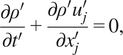
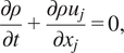 $$ \frac{\partial \rho }{\partial t}+\frac{\partial \rho {u}_j}{\partial {x}_j}=0, $$
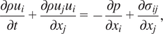 $$ \frac{\partial \rho {u}_i}{\partial t}+\frac{\partial \rho {u}_j{u}_i}{\partial {x}_j}=-\frac{\partial p}{\partial {x}_i}+\frac{\partial {\sigma}_{ij}}{\partial {x}_j}, $$
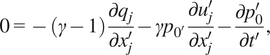
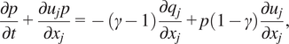 $$ \frac{\partial p}{\partial t}+\frac{\partial {u}_jp}{\partial {x}_j}=-\left(\gamma -1\right)\frac{\partial {q}_j}{\partial {x}_j}+p\left(1-\gamma \right)\frac{\partial {u}_j}{\partial {x}_j}, $$
 $$ p= r\rho T, $$
where
 $ \rho $
is the density,
$ \rho $
is the density,
 $ t $
the time,
$ t $
the time,
 $ p $
the pressure,
$ p $
the pressure,
 $ \gamma $
the adiabatic index of the fluid,
$ \gamma $
the adiabatic index of the fluid,
 $ r $
is the ideal gas-specific constant,
$ r $
is the ideal gas-specific constant,
 $ {u}_i $
the
$ {u}_i $
the
 $ i $
th component of velocity, and
$ i $
th component of velocity, and
 $ {x}_i $
the Cartesian coordinate in
$ {x}_i $
the Cartesian coordinate in
 $ i $
th direction. The shear-stress tensor
$ i $
th direction. The shear-stress tensor
 $ \sigma $
and the conductive heat flux
$ \sigma $
and the conductive heat flux
 $ \boldsymbol{q} $
are assumed to be of the form
$ \boldsymbol{q} $
are assumed to be of the form
 $ {\sigma}_{ij}=\mu (T)\left[\left({\partial}_j{u}_i+{\partial}_i{u}_j\right)-\left(2/3\right){\partial}_k{u}_k{\delta}_{ij}\right] $
and
$ {\sigma}_{ij}=\mu (T)\left[\left({\partial}_j{u}_i+{\partial}_i{u}_j\right)-\left(2/3\right){\partial}_k{u}_k{\delta}_{ij}\right] $
and
 $ {q}_j=-\lambda (T){\partial}_jT $
respectively, where the dynamic viscosity
$ {q}_j=-\lambda (T){\partial}_jT $
respectively, where the dynamic viscosity
 $ \mu (T) $
and the heat conductivity
$ \mu (T) $
and the heat conductivity
 $ \lambda (T) $
are functions of temperature. Dissipation has been neglected in the pressure evolution equation (5), as this term vanishes in the low Mach number limit (Paolucci, Reference Paolucci1982). The dynamic viscosity
$ \lambda (T) $
are functions of temperature. Dissipation has been neglected in the pressure evolution equation (5), as this term vanishes in the low Mach number limit (Paolucci, Reference Paolucci1982). The dynamic viscosity
 $ \mu (T) $
is monotonous increasing in terms of
$ \mu (T) $
is monotonous increasing in terms of
 $ T $
and separable,
$ T $
and separable,
 $ \mu (kT)={h}^{-1}(k)\mu (T) $
, which is for instance the case for a power law
$ \mu (kT)={h}^{-1}(k)\mu (T) $
, which is for instance the case for a power law
 $ \mu (T)={\mu}_0{\left(T/{T}_0\right)}^k $
. The thermal conductivity is given by
$ \mu (T)={\mu}_0{\left(T/{T}_0\right)}^k $
. The thermal conductivity is given by
 $ \lambda (T)=\mu (T){C}_p/\mathit{\Pr} $
, with
$ \lambda (T)=\mu (T){C}_p/\mathit{\Pr} $
, with
 $ {C}_p $
the isobaric heat capacity of the fluid and
$ {C}_p $
the isobaric heat capacity of the fluid and
 $ \mathit{\Pr} $
the Prandtl number of the fluid, both assumed constant. Suppose that this flow is characterized by a density scale
$ \mathit{\Pr} $
the Prandtl number of the fluid, both assumed constant. Suppose that this flow is characterized by a density scale
 $ {\rho}^b $
, a velocity scale
$ {\rho}^b $
, a velocity scale
 $ {u}^b $
, and a pressure scale
$ {u}^b $
, and a pressure scale
 $ {p}^b $
. The nondimensional numbers associated with the flow are the Reynolds number
$ {p}^b $
. The nondimensional numbers associated with the flow are the Reynolds number
 $ \mathit{\operatorname{Re}}={\rho}^b{u}^b{x}^b/\mu \left({T}^b\right) $
, the Prandtl number
$ \mathit{\operatorname{Re}}={\rho}^b{u}^b{x}^b/\mu \left({T}^b\right) $
, the Prandtl number
 $ \mathit{\Pr}=\mu \left({T}^b\right){C}_p/\lambda \left({T}^b\right) $
, and the Mach number
$ \mathit{\Pr}=\mu \left({T}^b\right){C}_p/\lambda \left({T}^b\right) $
, and the Mach number
 $ Ma={u}^b/{c}^b $
, with
$ Ma={u}^b/{c}^b $
, with
 $ {x}^b $
a length scale characterizing the geometry, and
$ {x}^b $
a length scale characterizing the geometry, and
 $ {c}^b=\sqrt{\gamma {rT}^b} $
the typical speed of sound.
$ {c}^b=\sqrt{\gamma {rT}^b} $
the typical speed of sound.
At the low Mach number limit, modifying the scales of the flows does not modify the flow in a nondimensional sense, provided that the Reynolds and Prandtl number are kept constant. Indeed, consider another similar flow with a different Mach number and different scales of length, velocity, and temperature but the same Reynolds and Prandtl number, as follows:
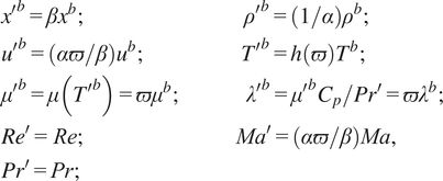 $$ {\displaystyle \begin{array}{l}{x^{\prime}}^b=\beta {x}^b;\hskip11.6em {\rho^{\prime}}^b=\left(1/\alpha \right){\rho}^b;\\ {}{u^{\prime}}^b=\left(\alpha \varpi /\beta \right){u}^b;\hskip7em {T^{\prime}}^b=h\left(\varpi \right){T}^b;\\ {}{\mu^{\prime}}^b=\mu \left({T^{\prime}}^b\right)={\varpi \mu}^b;\hskip4.8em {\lambda^{\prime}}^b={\mu^{\prime}}^b{C}_p/P{r}^{\prime }={\varpi \lambda}^b;\\ {}R{e}^{\prime }=\mathit{\operatorname{Re}};\hskip11em Ma^{\prime }=\left(\alpha \varpi /\beta \right) Ma,\\ {}P{r}^{\prime }=\mathit{\Pr};\end{array}} $$
where
 $ \alpha $
,
$ \alpha $
,
 $ \beta $
, and
$ \beta $
, and
 $ \varpi $
are constant scalars characterizing the transformation. At low Mach number, the nondimensionalized density and velocity are independent of the Mach number while the Mach number dependence of pressure cannot be neglected. Namely,
$ \varpi $
are constant scalars characterizing the transformation. At low Mach number, the nondimensionalized density and velocity are independent of the Mach number while the Mach number dependence of pressure cannot be neglected. Namely,
 $ u/{u}^b\approx {\hat{u}}_0 $
,
$ u/{u}^b\approx {\hat{u}}_0 $
,
 $ \rho /{\rho}^b\approx {\hat{\rho}}_0 $
and
$ \rho /{\rho}^b\approx {\hat{\rho}}_0 $
and
 $ p/{p}^b\approx {\hat{p}}_0+{Ma}^2{\hat{p}}_1 $
, where
$ p/{p}^b\approx {\hat{p}}_0+{Ma}^2{\hat{p}}_1 $
, where
 $ {\hat{u}}_0 $
,
$ {\hat{u}}_0 $
,
 $ {\hat{\rho}}_0 $
,
$ {\hat{\rho}}_0 $
,
 $ {\hat{p}}_0 $
, and
$ {\hat{p}}_0 $
, and
 $ {\hat{p}}_1 $
do not depend on the Mach number (Lions and Moulden, Reference Lions and Moulden1996; Meister, Reference Meister1999; Munz et al., Reference Munz, Dumbser and Zucchini2003). The zeroth-order nondimensionalized pressure
$ {\hat{p}}_1 $
do not depend on the Mach number (Lions and Moulden, Reference Lions and Moulden1996; Meister, Reference Meister1999; Munz et al., Reference Munz, Dumbser and Zucchini2003). The zeroth-order nondimensionalized pressure
 $ {\hat{p}}_0 $
can be shown to be constant in space by injecting these asymptotic developments into the Navier–Stokes equations. It is therefore useful to decompose pressure in a thermodynamical pressure
$ {\hat{p}}_0 $
can be shown to be constant in space by injecting these asymptotic developments into the Navier–Stokes equations. It is therefore useful to decompose pressure in a thermodynamical pressure
 $ {p}_0={p}^b{\hat{p}}_0 $
and a mechanical pressure
$ {p}_0={p}^b{\hat{p}}_0 $
and a mechanical pressure
 $ {p}_1=p-{p}_0={p}^b{Ma}^2{\hat{p}}_1 $
. Hence, the thermodynamical and mechanical pressures are given by
$ {p}_1=p-{p}_0={p}^b{Ma}^2{\hat{p}}_1 $
. Hence, the thermodynamical and mechanical pressures are given by
 $ {p}_0^{\prime }={p^{\prime}}^b{\hat{p}}_0=\left(h\left(\varpi \right)/\alpha \right){p}_0 $
and
$ {p}_0^{\prime }={p^{\prime}}^b{\hat{p}}_0=\left(h\left(\varpi \right)/\alpha \right){p}_0 $
and
 $ {p}_1^{\prime }={p^{\prime}}^b{\alpha}^2{Ma}^2{\hat{p}}_1=\left({\alpha \varpi}^2/{\beta}^2\right){p}_1 $
.
$ {p}_1^{\prime }={p^{\prime}}^b{\alpha}^2{Ma}^2{\hat{p}}_1=\left({\alpha \varpi}^2/{\beta}^2\right){p}_1 $
.
Based on these insights, let us consider the change of variables
 $ x=\left(1/\beta \right){x}^{\prime } $
,
$ x=\left(1/\beta \right){x}^{\prime } $
,
 $ t=\left(\alpha \varpi /{\beta}^2\right){t}^{\prime } $
,
$ t=\left(\alpha \varpi /{\beta}^2\right){t}^{\prime } $
,
 $ u={u}^{\prime}\beta /\left(\alpha \varpi \right) $
,
$ u={u}^{\prime}\beta /\left(\alpha \varpi \right) $
,
 $ \rho =\alpha {\rho}^{\prime } $
,
$ \rho =\alpha {\rho}^{\prime } $
,
 $ {p}_0=\left(\alpha /h\left(\varpi \right)\right){p}_0^{\prime } $
,
$ {p}_0=\left(\alpha /h\left(\varpi \right)\right){p}_0^{\prime } $
,
 $ {p}_1={p}_1^{\prime }{\beta}^2/\left({\alpha \varpi}^2\right) $
,
$ {p}_1={p}_1^{\prime }{\beta}^2/\left({\alpha \varpi}^2\right) $
,
 $ T=\left(1/h\left(\varpi \right)\right){T}^{\prime } $
,
$ T=\left(1/h\left(\varpi \right)\right){T}^{\prime } $
,
 $ \mu ={\mu}^{\prime }/\varpi $
, and
$ \mu ={\mu}^{\prime }/\varpi $
, and
 $ \lambda ={\lambda}^{\prime }/\varpi $
. Hereafter, we refer to this change of variable as a Mach-number transformation, since this change of variable modifies the Mach number of the flow. Introducing the change of variables in equations (3)–(6) leads to:
$ \lambda ={\lambda}^{\prime }/\varpi $
. Hereafter, we refer to this change of variable as a Mach-number transformation, since this change of variable modifies the Mach number of the flow. Introducing the change of variables in equations (3)–(6) leads to:
 $$ \frac{\partial {\rho}^{\prime }}{\partial {t}^{\prime }}+\frac{\partial {\rho}^{\prime }{u}_j^{\prime }}{\partial {x}_j^{\prime }}=0, $$
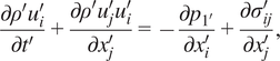 $$ \frac{\partial {\rho}^{\prime }{u}_i^{\prime }}{\partial {t}^{\prime }}+\frac{\partial {\rho}^{\prime }{u}_j^{\prime }{u}_i^{\prime }}{\partial {x}_j^{\prime }}=-\frac{\partial {p}_{1^{\prime }}}{\partial {x}_i^{\prime }}+\frac{\partial {\sigma}_{ij}^{\prime }}{\partial {x}_j^{\prime }}, $$
 $$ \frac{\partial {p}_1^{\prime }}{\partial {t}^{\prime }}+\frac{\partial {u}_j^{\prime }{p}_1^{\prime }}{\partial {x}_j^{\prime }}=-\left(\gamma -1\right)\frac{\alpha^2{\varpi}^2}{h\left(\varpi \right){\beta}^2}\frac{\partial {q}_j}{\partial {x}_j^{\prime }}+\left({p}_1^{\prime}\left(1-\gamma \right)-\gamma {p}_0^{\prime}\frac{\alpha^2{\varpi}^2}{h\left(\varpi \right){\beta}^2}\right)\frac{\partial {u}_j^{\prime }}{\partial {x}_j^{\prime }}-\frac{\alpha^2{\varpi}^2}{h\left(\varpi \right){\beta}^2}\frac{\partial {p}_0^{\prime }}{\partial {t}^{\prime }}, $$
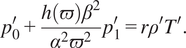 $$ {p}_0^{\prime }+\frac{h\left(\varpi \right){\beta}^2}{\alpha^2{\varpi}^2}{p}_1^{\prime }=r{\rho}^{\prime }{T}^{\prime }. $$
At the limit of a low Mach number, the terms involving
 $ {p}_1^{\prime } $
in equations (9) and (10) vanish and the system of equations (7)–(10) tends to the low Mach number equations of Paolucci (Reference Paolucci1982):
$ {p}_1^{\prime } $
in equations (9) and (10) vanish and the system of equations (7)–(10) tends to the low Mach number equations of Paolucci (Reference Paolucci1982):
 $$ \frac{\partial {\rho}^{\prime }}{\partial {t}^{\prime }}+\frac{\partial {\rho}^{\prime }{u}_j^{\prime }}{\partial {x}_j^{\prime }}=0, $$
 $$ \frac{\partial {\rho}^{\prime }{u}_i^{\prime }}{\partial {t}^{\prime }}+\frac{\partial {\rho}^{\prime }{u}_j^{\prime }{u}_i^{\prime }}{\partial {x}_j^{\prime }}=-\frac{\partial {p}_1^{\prime }}{\partial {x}_i^{\prime }}+\frac{\partial {\sigma}_{ij}^{\prime }}{\partial {x}_j^{\prime }}, $$
 $$ 0=-\left(\gamma -1\right)\frac{\partial {q}_j}{\partial {x}_j^{\prime }}-\gamma {p}_{0^{\prime }}\frac{\partial {u}_j^{\prime }}{\partial {x}_j^{\prime }}-\frac{\partial {p}_0^{\prime }}{\partial {t}^{\prime }}, $$
 $$ {p}_0^{\prime }=r{\rho}^{\prime }{T}^{\prime }. $$
This system of equations does not depend on any of the scalar parameters
 $ \alpha $
,
$ \alpha $
,
 $ \beta $
, or
$ \beta $
, or
 $ \varpi $
. Hence, the Mach-number transformation is parameterized by
$ \varpi $
. Hence, the Mach-number transformation is parameterized by
 $ \alpha $
,
$ \alpha $
,
 $ \beta $
, and
$ \beta $
, and
 $ \varpi $
does not modify the system of equations. It follows that the solution of the system of equations (11)–(14) with different scales of velocity, density, viscosity, and length can be deduced from such transformation.
$ \varpi $
does not modify the system of equations. It follows that the solution of the system of equations (11)–(14) with different scales of velocity, density, viscosity, and length can be deduced from such transformation.
To summarize, a relevant corollary with respect to the machine learning model is that under a Mach-number transformation of its the input features,
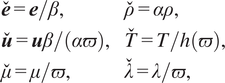 $$ {\displaystyle \begin{array}{ll}\overset{\check{}}{\boldsymbol{e}}=\boldsymbol{e}/\beta, & \overset{\check{}}{\rho }=\alpha \rho, \\ {}\overset{\check{}}{\boldsymbol{u}}=\boldsymbol{u}\beta /\left(\alpha \varpi \right),& \overset{\check{}}{T}=T/h\left(\varpi \right),\\ {}\overset{\check{}}{\mu }=\mu /\varpi, & \overset{\check{}}{\lambda }=\lambda /\varpi, \end{array}} $$
the model’s prediction should undergo the same transformation. Namely, the norm of the shear stress vector
 $ \tau =\Sigma \cdot {\boldsymbol{e}}_{\boldsymbol{n}}-\left({\boldsymbol{e}}_{\boldsymbol{n}}\cdot \Sigma \cdot {\boldsymbol{e}}_{\boldsymbol{n}}\right){\boldsymbol{e}}_{\boldsymbol{n}} $
, where
$ \tau =\Sigma \cdot {\boldsymbol{e}}_{\boldsymbol{n}}-\left({\boldsymbol{e}}_{\boldsymbol{n}}\cdot \Sigma \cdot {\boldsymbol{e}}_{\boldsymbol{n}}\right){\boldsymbol{e}}_{\boldsymbol{n}} $
, where
 $ \Sigma =\mu \left(\nabla \boldsymbol{u}+{\left(\nabla \boldsymbol{u}\right)}^T-\left(2/3\right)\left(\nabla \cdot \boldsymbol{u}\right){\mathbf{I}}_{\mathbf{d}}\right) $
is the viscous stress tensor and
$ \Sigma =\mu \left(\nabla \boldsymbol{u}+{\left(\nabla \boldsymbol{u}\right)}^T-\left(2/3\right)\left(\nabla \cdot \boldsymbol{u}\right){\mathbf{I}}_{\mathbf{d}}\right) $
is the viscous stress tensor and
 $ {\boldsymbol{e}}_{\boldsymbol{n}} $
a unit wall-normal vector, and the norm of the heat flux at the wall should undergo the transformation
$ {\boldsymbol{e}}_{\boldsymbol{n}} $
a unit wall-normal vector, and the norm of the heat flux at the wall should undergo the transformation
 $$ \hskip0.5em \overset{\check{}}{\tau }=\alpha \tau {\left(\beta /\left(\alpha \varpi \right)\right)}^2,\hskip1.00em \overset{\check{}}{q}= q\beta /\left(\varpi h\left(\varpi \right)\right). $$
This property will thereupon will be referred to as the Mach-number equivariance of the model. Particular cases of the Mach-number transformation are the
 $ \alpha $
-transformation,
$ \alpha $
-transformation,
 $ \beta $
-transformation, and
$ \beta $
-transformation, and
 $ \varpi $
-transformation, which respectively correspond to
$ \varpi $
-transformation, which respectively correspond to
 $ \beta =\varpi =1 $
,
$ \beta =\varpi =1 $
,
 $ \alpha =\varpi =1 $
, and
$ \alpha =\varpi =1 $
, and
 $ \alpha =\beta =1 $
. The equivariance of the model under a Mach-number transformation is not exact for real flows, including the flows in the numerical database, as it relies on several approximations, most notably that of a low Mach number and constant adiabatic index. It is nevertheless useful to introduce this approximate equivariance in the learning process to build with limited data a model that can generalize to flows with different scales of velocity, density, viscosity, and length. The a priori results should demonstrate that these approximations are not critical for the performance of the model.
$ \alpha =\beta =1 $
. The equivariance of the model under a Mach-number transformation is not exact for real flows, including the flows in the numerical database, as it relies on several approximations, most notably that of a low Mach number and constant adiabatic index. It is nevertheless useful to introduce this approximate equivariance in the learning process to build with limited data a model that can generalize to flows with different scales of velocity, density, viscosity, and length. The a priori results should demonstrate that these approximations are not critical for the performance of the model.
3.2. Strategies for equivariance enforcement
There are at least to two ways to leverage the equivariance of the model to a transformation
 $ \mathcal{P} $
within the training process: the invariant feature strategy and the data-augmentation strategy. In the invariant-feature strategy, the model is expressed in terms of invariant trainable functions by algorithmically constructing invariant features from the input data
$ \mathcal{P} $
within the training process: the invariant feature strategy and the data-augmentation strategy. In the invariant-feature strategy, the model is expressed in terms of invariant trainable functions by algorithmically constructing invariant features from the input data
 $ \boldsymbol{X} $
(Villar et al., Reference Villar, Storey-Fisher, Yao and Blum-Smith2021, Reference Villar, Yao, Hogg, Blum-Smith and Dumitrascu2022). One particular way to construct these invariant features is to use a reference to restrict the input space of the model. For instance, a privileged direction and an intrinsic velocity reference can be used to enforce rotational invariance and Galilean equivariance respectively. For machine-learning wall modeling, the wall may provide such references for the
$ \boldsymbol{X} $
(Villar et al., Reference Villar, Storey-Fisher, Yao and Blum-Smith2021, Reference Villar, Yao, Hogg, Blum-Smith and Dumitrascu2022). One particular way to construct these invariant features is to use a reference to restrict the input space of the model. For instance, a privileged direction and an intrinsic velocity reference can be used to enforce rotational invariance and Galilean equivariance respectively. For machine-learning wall modeling, the wall may provide such references for the
 $ \alpha $
- and
$ \alpha $
- and
 $ \varpi $
-transformations. In the data-augmentation strategy, the input space of the model is increased by using the transformation
$ \varpi $
-transformations. In the data-augmentation strategy, the input space of the model is increased by using the transformation
 $ \mathcal{P} $
to create modified copies of the training samples. For instance, arbitrary rotations and translations can be used to enforce rotational invariance and Galilean equivariance respectively. The two strategies are represented schematically in Figure 1. The invariant-feature strategy is generally more costly than the data augmentation in terms of training time. However, it adds a pre-processing and post-processing step to the model at inference time, which may hinder its implementation in a CFD code.
$ \mathcal{P} $
to create modified copies of the training samples. For instance, arbitrary rotations and translations can be used to enforce rotational invariance and Galilean equivariance respectively. The two strategies are represented schematically in Figure 1. The invariant-feature strategy is generally more costly than the data augmentation in terms of training time. However, it adds a pre-processing and post-processing step to the model at inference time, which may hinder its implementation in a CFD code.
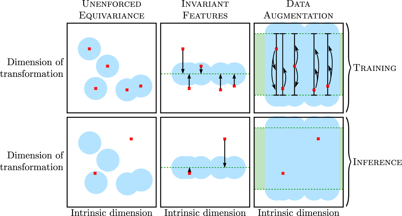
Figure 1. Schematic representation of the scaling and data augmentation strategies, where the input space is formally decomposed into the dimension of a transformation
 $ \mathcal{P} $
, with respect to which the model is assumed equivariant, and an intrinsic dimension, which represents of the physical content of the input data, invariant under
$ \mathcal{P} $
, with respect to which the model is assumed equivariant, and an intrinsic dimension, which represents of the physical content of the input data, invariant under
 $ \mathcal{P} $
. The red crosses represent different simulations seen during training or at inference time. The blue areas are the portion of input space seen during training, which for illustrative purpose is assumed to be a sphere in the feature space.
$ \mathcal{P} $
. The red crosses represent different simulations seen during training or at inference time. The blue areas are the portion of input space seen during training, which for illustrative purpose is assumed to be a sphere in the feature space.
In the present study, the equivariance of the model under an orthogonal transformation, a Galilean transformation, and the
 $ \alpha $
-,
$ \alpha $
-,
 $ \beta $
-, and
$ \beta $
-, and
 $ \varpi $
-transformations defined in Section 3.1 are considered. Since the walls are assumed to be isothermal, the dynamic viscosity is constant at the walls assuming that dynamic viscosity is only function of temperature. Accordingly, it is straightforward to define a
$ \varpi $
-transformations defined in Section 3.1 are considered. Since the walls are assumed to be isothermal, the dynamic viscosity is constant at the walls assuming that dynamic viscosity is only function of temperature. Accordingly, it is straightforward to define a
 $ \varpi $
-transformation that scales dynamic viscosity. In contrast, the wall density may vary due to variations of pressure and accordingly, it is difficult to equivocally select a particular value of the wall density to define an
$ \varpi $
-transformation that scales dynamic viscosity. In contrast, the wall density may vary due to variations of pressure and accordingly, it is difficult to equivocally select a particular value of the wall density to define an
 $ \alpha $
-transformation that scales density. Indeed, the density at each grid point is used for predictions at several wall locations. In light of the above, a strategy based on data augmentation has been selected to impose the equivariance of the model under a
$ \alpha $
-transformation that scales density. Indeed, the density at each grid point is used for predictions at several wall locations. In light of the above, a strategy based on data augmentation has been selected to impose the equivariance of the model under a
 $ \varpi $
-transformation while a strategy based on the scaling of input features has been selected to impose the equivariance of the model under an
$ \varpi $
-transformation while a strategy based on the scaling of input features has been selected to impose the equivariance of the model under an
 $ \alpha $
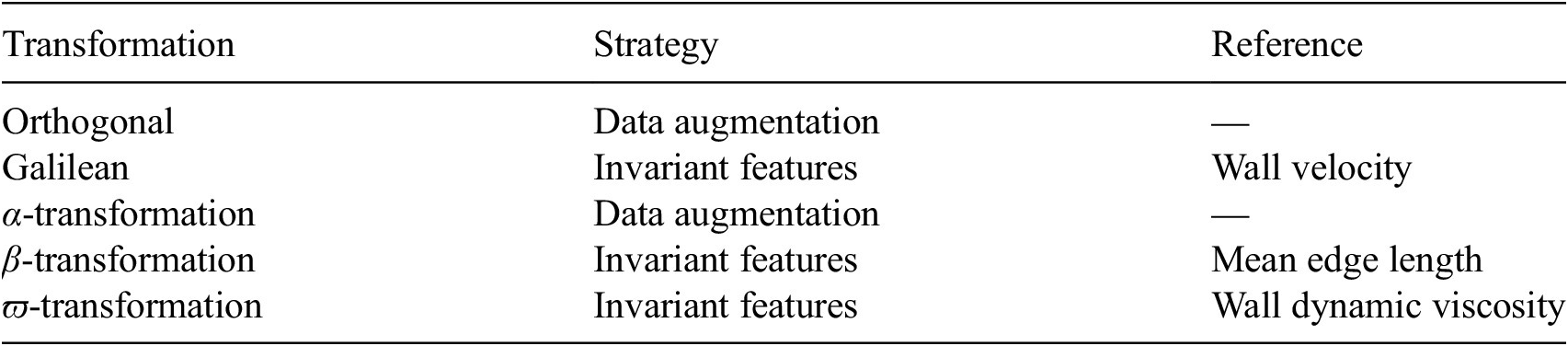
-transformation. Data augmentation is also used to ensure that the prediction of the model does not depend on the coordinate system. Table 2 summarizes the strategy used to enforce the equivariance of the model under each transformation considered:
$ \alpha $
-transformation. Data augmentation is also used to ensure that the prediction of the model does not depend on the coordinate system. Table 2 summarizes the strategy used to enforce the equivariance of the model under each transformation considered:
-
• Orthogonal equivariance is ensured by augmenting the dataset with arbitrary three-dimensional rotations and reflections of the axes.
-
• Galilean equivariance is ensured by expressing the input velocity relatively to the wall motion.
-
•
$ \alpha $
-equivariance is ensured by augmenting the dataset with arbitrary
$ \alpha $
-transformations, with
$ \alpha $
sampled from the log-uniform distribution with range
$ \left[{\rho}_{\mathrm{min}}/{\left\langle \rho \right\rangle}_{\mathfrak{W}},{\rho}_{\mathrm{max}}/{\left\langle \rho \right\rangle}_{\mathfrak{W}}\right] $
, where
$ {\left\langle \parallel \rho \parallel \right\rangle}_{\mathfrak{W}} $
is the mean wall density and where
$ \left[{\rho}_{\mathrm{min}},{\rho}_{\mathrm{max}}\right] $
is the desired density range of the model. -
•
$ \beta $
-equivariance is ensured by scaling the input data using the average edge length of the graph, denoted
$ {\left\langle \parallel \boldsymbol{e}\parallel \right\rangle}_{\mathfrak{G}} $
, that is by applying a
$ \beta $
-transformation with
$ \beta ={\left\langle \parallel \boldsymbol{e}\parallel \right\rangle}_{\mathfrak{G}} $
. -
•
$ \varpi $
-equivariance is ensured by scaling the input data using the wall dynamic viscosity
$ {\mu}_{\mathrm{wall}} $
, that is by applying a
$ \varpi $
-transformation with
$ \varpi ={\mu}_{\mathrm{wall}} $
.


Table 2. Strategies used to enforce the equivariance of the machine-learning model to various transformations, and references used to compute the scalings
For ease of interpretation, notice that the scaled input velocity may be expressed as
 $ \overset{\check{}}{\boldsymbol{u}}={\overset{\check{}}{\boldsymbol{u}}}^{+}{\left\langle \parallel {\boldsymbol{e}}^{+}\parallel \right\rangle}_{\mathfrak{G}}/\left({\alpha \rho}_{\mathrm{wall}}\right) $
, the scaled target wall shear stress as
$ \overset{\check{}}{\boldsymbol{u}}={\overset{\check{}}{\boldsymbol{u}}}^{+}{\left\langle \parallel {\boldsymbol{e}}^{+}\parallel \right\rangle}_{\mathfrak{G}}/\left({\alpha \rho}_{\mathrm{wall}}\right) $
, the scaled target wall shear stress as
 $ \overset{\check{}}{\tau }={\left\langle \parallel {\boldsymbol{e}}^{+}\parallel \right\rangle}_{\mathfrak{G}}^2/\left({\alpha \rho}_{\mathrm{wall}}\right) $
and the scaled wall heat flux
$ \overset{\check{}}{\tau }={\left\langle \parallel {\boldsymbol{e}}^{+}\parallel \right\rangle}_{\mathfrak{G}}^2/\left({\alpha \rho}_{\mathrm{wall}}\right) $
and the scaled wall heat flux
 $ \overset{\check{}}{q} $
is proportional to
$ \overset{\check{}}{q} $
is proportional to
 $ Cp\left(\left(\overset{\check{}}{T}-{\overset{\check{}}{T}}_{\mathrm{wall}}\right)/{\overset{\check{}}{T}}_{\mathrm{wall}}\right){\left\langle \parallel {\boldsymbol{e}}^{+}\parallel \right\rangle}_{\mathfrak{G}}/{T}^{+} $
, where
$ Cp\left(\left(\overset{\check{}}{T}-{\overset{\check{}}{T}}_{\mathrm{wall}}\right)/{\overset{\check{}}{T}}_{\mathrm{wall}}\right){\left\langle \parallel {\boldsymbol{e}}^{+}\parallel \right\rangle}_{\mathfrak{G}}/{T}^{+} $
, where
 $ {}^{+} $
denotes the classical wall-unit scaling, namely
$ {}^{+} $
denotes the classical wall-unit scaling, namely
 $ {e}^{+}={eu}_{\tau }/{\nu}_{\omega } $
,
$ {e}^{+}={eu}_{\tau }/{\nu}_{\omega } $
,
 $ {\boldsymbol{u}}^{+}=\boldsymbol{u}/{u}_{\tau } $
, and
$ {\boldsymbol{u}}^{+}=\boldsymbol{u}/{u}_{\tau } $
, and
 $ {T}^{+}={\rho}_{\omega }{C}_p{u}_{\tau}\left(T-{T}_{\mathrm{wall}}\right)/q $
. This scaling uniformizes the length scale of the various simulations included in the training database, but it does not negate differences in terms of mesh resolution, which implies that ideally a wide range of mesh resolution need to be included in the training dataset. Similarly, the scaling uniformizes the viscosity scale of the various simulations included in the training database, but it does not negate differences in terms of viscosity ratio between the wall and bulk flow, which implies that ideally a wide range of such viscosity ratio should be found in the training dataset.
$ {T}^{+}={\rho}_{\omega }{C}_p{u}_{\tau}\left(T-{T}_{\mathrm{wall}}\right)/q $
. This scaling uniformizes the length scale of the various simulations included in the training database, but it does not negate differences in terms of mesh resolution, which implies that ideally a wide range of mesh resolution need to be included in the training dataset. Similarly, the scaling uniformizes the viscosity scale of the various simulations included in the training database, but it does not negate differences in terms of viscosity ratio between the wall and bulk flow, which implies that ideally a wide range of such viscosity ratio should be found in the training dataset.
4. Wall modeling
This section presents the architecture of the graph neural network wall model and the algebraic wall models used as baselines.
4.1. Baseline wall models
Two algebraic wall models are used as baselines: an uncoupled velocity-temperature algebraic wall model and the coupled velocity-temperature algebraic wall model of Cabrit and Nicoud (Reference Cabrit and Nicoud2009).
The uncoupled algebraic wall model provides a boundary condition for the wall shear stress and the wall conductive heat flux without taking into account the coupling between the velocity and temperature profiles. Namely, the wall shear stress is obtained by solving the incompressible law of the wall,
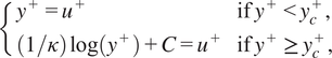 $$ \left\{\begin{array}{ll}{y}^{+}={u}^{+}& \mathrm{if}\;{y}^{+}<{y}_c^{+},\\ {}\left(1/\kappa \right)\log \left({y}^{+}\right)+C={u}^{+}& \mathrm{if}\;{y}^{+}\ge {y}_c^{+},\end{array}\right. $$
and the wall heat flux is obtained by solving the temperature law
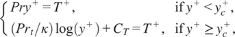 $$ \left\{\begin{array}{ll}{Pry}^{+}={T}^{+},& \mathrm{if}\;{y}^{+}<{y}_c^{+},\\ {}\left({\mathit{\Pr}}_t/\kappa \right)\log \left({y}^{+}\right)+{C}_T={T}^{+},& \mathrm{if}\;{y}^{+}\ge {y}_c^{+},\end{array}\right. $$
with
 $ \kappa =0.41 $
the von Kármán constant,
$ \kappa =0.41 $
the von Kármán constant,
 $ C=5.5 $
a scalar constant,
$ C=5.5 $
a scalar constant,
 $ {\mathit{\Pr}}_t=0.85 $
the turbulent Prandtl number and
$ {\mathit{\Pr}}_t=0.85 $
the turbulent Prandtl number and
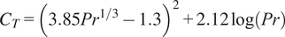 $$ {C}_T={\left(3.85{\mathit{\Pr}}^{1/3}-1.3\right)}^2+2.12\log \left(\mathit{\Pr}\right) $$
a function of the Prandtl number (Kader, Reference Kader1981). The threshold
 $ {y}_c^{+}=11.445 $
is a critical value of the scaled first point height separating the viscous and inertial sublayers. The scaled wall distance is
$ {y}_c^{+}=11.445 $
is a critical value of the scaled first point height separating the viscous and inertial sublayers. The scaled wall distance is
 $ {y}^{+}={yu}_{\tau }/{\nu}_{\omega } $
, the scaled temperature
$ {y}^{+}={yu}_{\tau }/{\nu}_{\omega } $
, the scaled temperature
 $ {T}^{+}=\left(T-{T}_{\omega}\right)/{T}_{\tau } $
and the scaled velocity
$ {T}^{+}=\left(T-{T}_{\omega}\right)/{T}_{\tau } $
and the scaled velocity
 $ {u}^{+}=u/{u}_{\tau } $
. The wall shear stress and conductive heat flux are solved sequentially from equations (17) then (18) and the friction velocity and friction temperature definitions, namely
$ {u}^{+}=u/{u}_{\tau } $
. The wall shear stress and conductive heat flux are solved sequentially from equations (17) then (18) and the friction velocity and friction temperature definitions, namely
 $ \tau ={\rho}_{\omega }{u}_{\tau}^2 $
and
$ \tau ={\rho}_{\omega }{u}_{\tau}^2 $
and
 $ {q}_{\omega }={\rho}_{\omega }{C}_p{u}_{\tau }{T}_{\tau } $
. The uncoupled algebraic model does not take into account the effect of the temperature variations to determine the wall shear stress. It is commonly used and accurate in flows with a negligible coupling between the fields of velocity and temperature, for example, when the temperature variations are not large.
$ {q}_{\omega }={\rho}_{\omega }{C}_p{u}_{\tau }{T}_{\tau } $
. The uncoupled algebraic model does not take into account the effect of the temperature variations to determine the wall shear stress. It is commonly used and accurate in flows with a negligible coupling between the fields of velocity and temperature, for example, when the temperature variations are not large.
The coupled algebraic wall model of Cabrit and Nicoud (Reference Cabrit and Nicoud2009) is an algebraic model that takes into account the coupling between the fields of velocity and temperature. In the case of a compressible non-reacting flow, the coupled wall model of Cabrit and Nicoud (Reference Cabrit and Nicoud2009) may be expressed by the following system of equations.
-
• Velocity equation:
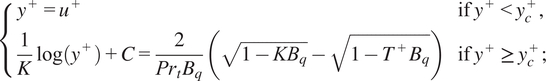 $$ \left\{\begin{array}{ll}{y}^{+}={u}^{+}& \mathrm{if}\;{y}^{+}<{y}_c^{+},\\ {}\frac{1}{K}\log \left({y}^{+}\right)+C=\frac{2}{{\mathit{\Pr}}_t{B}_q}\left(\sqrt{1-{KB}_q}-\sqrt{1-{T}^{+}{B}_q}\right)& \mathrm{if}\;{y}^{+}\ge {y}_c^{+};\end{array}\right. $$
-
• Temperature equation:
 $$ {\mathit{\Pr}}_t{u}^{+}+K={T}^{+}; $$
with
 $ {B}_q={T}_{\tau }/{T}_{\omega } $
the anisothermicity factor, and
$ {B}_q={T}_{\tau }/{T}_{\omega } $
the anisothermicity factor, and
 $ K $
a function of the Prandtl number, given by
$ K $
a function of the Prandtl number, given by
 $$ K={C}_T-{\mathit{\Pr}}_tC+\left(\frac{{\mathit{\Pr}}_t}{\kappa }-2.12\right)\left(1-2\log (20)\right), $$
where
 $ {C}_T $
is defined in equation (19). To solve this system of equations, a candidate friction velocity is first computed by injecting
$ {C}_T $
is defined in equation (19). To solve this system of equations, a candidate friction velocity is first computed by injecting
 $ {y}^{+}={yu}_{\tau }/{\nu}_{\omega } $
and
$ {y}^{+}={yu}_{\tau }/{\nu}_{\omega } $
and
 $ {T}^{+}=\left(T-{T}_{\omega}\right)/{T}_{\tau } $
in equation (2
1). This candidate value is discarded if the corresponding scaled first point height
$ {T}^{+}=\left(T-{T}_{\omega}\right)/{T}_{\tau } $
in equation (2
1). This candidate value is discarded if the corresponding scaled first point height
 $ {y}^{+} $
is less than
$ {y}^{+} $
is less than
 $ {y}_c^{+} $
, in which case
$ {y}_c^{+} $
, in which case
 $ {u}_{\tau } $
is solved using (20). In any case, the friction temperature
$ {u}_{\tau } $
is solved using (20). In any case, the friction temperature
 $ {T}_{\tau } $
is then computed by injecting
$ {T}_{\tau } $
is then computed by injecting
 $ {u}^{+}=u/{u}_{\tau } $
in equation (22). The wall shear stress and conductive heat flux are deduced from the friction velocity and temperature definitions, namely
$ {u}^{+}=u/{u}_{\tau } $
in equation (22). The wall shear stress and conductive heat flux are deduced from the friction velocity and temperature definitions, namely
 $ \tau ={\rho}_{\omega }{u}_{\tau}^2 $
and
$ \tau ={\rho}_{\omega }{u}_{\tau}^2 $
and
 $ {q}_{\omega }={\rho}_{\omega }{C}_p{u}_{\tau }{T}_{\tau } $
. The coupled algebraic model of Cabrit and Nicoud (Reference Cabrit and Nicoud2009) takes into account the effect of the temperature variations to determine the wall shear stress. It is relevant for fully developed turbulent boundary layers with large temperature variations.
$ {q}_{\omega }={\rho}_{\omega }{C}_p{u}_{\tau }{T}_{\tau } $
. The coupled algebraic model of Cabrit and Nicoud (Reference Cabrit and Nicoud2009) takes into account the effect of the temperature variations to determine the wall shear stress. It is relevant for fully developed turbulent boundary layers with large temperature variations.
4.2. Graph neural network wall model
A graph neural network is a class of artificial neural network designed to process graph-structured data, that is a set of nodes and edges along with, optionally, node-valued or edge-valued fields. In the present work, the “graph” corresponds to the numerical fields of an unstructured-mesh simulation. The nodes of the graph are given by the nodes of the mesh. The edges of the graph are given by the edges of the mesh, or in other words the mesh connectivity. The present graph neural network wall model uses the Encode-Process-Decode architecture of Battaglia et al. (Reference Battaglia, Hamrick, Bapst, Sanchez-Gonzalez, Zambaldi, Malinowski, Tacchetti, Raposo, Santoro, Faulkner, Gulcehre, Song, Ballard, Gilmer, Dahl, Vaswani, Allen, Nash, Langston, Dyer, Heess, Wierstra, Kohli, Botvinick, Vinyals, Li and Pascanu2018) and Dupuy et al. (Reference Dupuy, Odier, Lapeyre and Papadogiannis2023b), represented schematically in Figure 2. This architecture has been selected for its ability to directly operate on the unstructured data of the simulation, without requiring the prior interpolation of the inputs. The method is owing to this property easily applicable in LESs of complex geometries, with angles, corners, or curvature. Furthermore, the architecture implicitly makes some physical assumptions that are relevant for the modeling of the wall shear stress or wall heat flux. Namely, the prediction is invariant under a translation of the computational domain and biased toward locality, meaning that the model will more easily use nearby spatial locations for its prediction than far-away locations. The model will be trained to operate on mesh-based data, and produce a field of the wall shear stress or the wall conductive heat flux. To this end, it will leverage the inherent spatial relationships and dependencies found in the training database. Note that while the present approach does not incorporate specific physical laws or equations as in the case of physics-informed neural networks (PINN, (Raissi et al., Reference Raissi, Perdikaris and Karniadakis2019), it is not purely data-based since it is combined with scaling and data augmentation techniques presented in Section 3.2 to improve the generalizability of the model to other scales of length, velocity, temperature or pressure, and encode relevant physical equivariances. Due to this, the model will encode the physical assumptions of Galilean invariance, orthogonal equivariance that is the equivariance under a rotation or reflection of the computational domain, and Mach-number equivariance that is the equivariance under a change of scale that can be made under the assumption of a low Mach number. We accordingly assume that the effect of the Mach number on the boundary layer is not too large, which excludes hypersonic flows from the domain of applicability of the method. Finally, we assume that the Prandtl number of the flow is constant and that the variations of adiabatic index can be neglected for the temperature range of the flow.
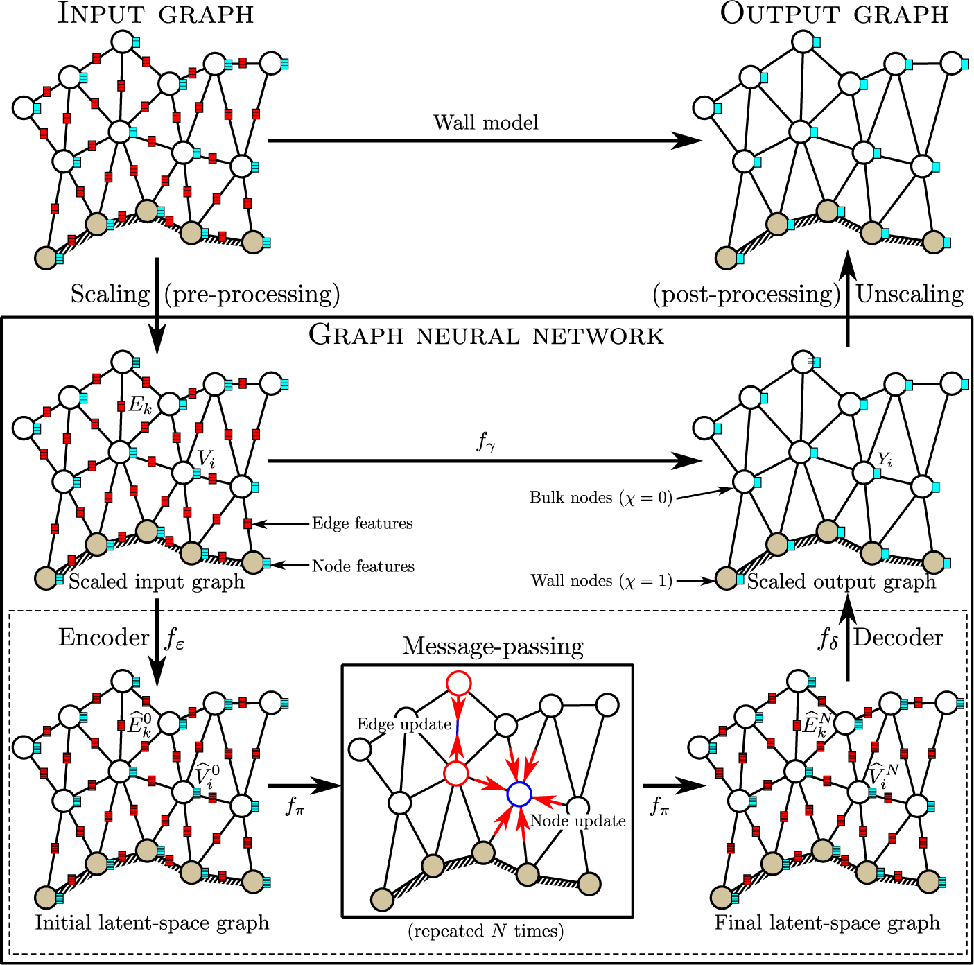
Figure 2. Graphical representation of the Encode-Process-Decode architecture. The scaling (pre-processing) and unscaling (post-processing) steps correspond to the transformations as listed in Table 2.
The model architecture may be described as follows. The input of the model
 $ \boldsymbol{X} $
is first encoded into a latent space, processed iteratively by
$ \boldsymbol{X} $
is first encoded into a latent space, processed iteratively by
 $ N $
identical message-passing steps, and finally decoded back to physical space to produce the output
$ N $
identical message-passing steps, and finally decoded back to physical space to produce the output
 $ \boldsymbol{Y} $
:
$ \boldsymbol{Y} $
:
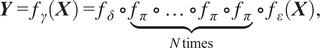 $$ \boldsymbol{Y}={f}_{\gamma}\left(\boldsymbol{X}\right)={f}_{\delta}\hskip0.35em \circ \hskip0.35em \underset{N\;\mathrm{times}}{\underbrace{f_{\pi}\hskip0.35em \circ \hskip0.35em \dots \hskip0.35em \circ \hskip0.35em {f}_{\pi}\hskip0.35em \circ \hskip0.35em {f}_{\pi }}}\hskip0.35em \circ \hskip0.35em {f}_{\varepsilon}\left(\boldsymbol{X}\right), $$
where
 $ {f}_{\varepsilon } $
,
$ {f}_{\varepsilon } $
,
 $ {f}_{\pi } $
, and
$ {f}_{\pi } $
, and
 $ {f}_{\delta } $
are learned functions associated respectively with the encoding, processing, and decoding steps. The model input
$ {f}_{\delta } $
are learned functions associated respectively with the encoding, processing, and decoding steps. The model input
 $ \boldsymbol{X} $
is represented as a symmetric directed graph valued at both edges and nodes. Namely, it is an ordered pair
$ \boldsymbol{X} $
is represented as a symmetric directed graph valued at both edges and nodes. Namely, it is an ordered pair
 $ \boldsymbol{X}=\left(\boldsymbol{V},\boldsymbol{E}\right) $
, where
$ \boldsymbol{X}=\left(\boldsymbol{V},\boldsymbol{E}\right) $
, where
 $ \boldsymbol{V} $
is the vector of the input features at the nodes of the graph and
$ \boldsymbol{V} $
is the vector of the input features at the nodes of the graph and
 $ \boldsymbol{E} $
the vector of the input features at the edges of the graph. The encoder
$ \boldsymbol{E} $
the vector of the input features at the edges of the graph. The encoder
 $ {f}_{\varepsilon } $
is a set of two multilayer perceptrons
$ {f}_{\varepsilon } $
is a set of two multilayer perceptrons
 $ {f}_{\varepsilon}^V $
and
$ {f}_{\varepsilon}^V $
and
 $ {f}_{\varepsilon}^E $
that upscale the features at each edge or node independently. Specifically, the encoded feature
$ {f}_{\varepsilon}^E $
that upscale the features at each edge or node independently. Specifically, the encoded feature
 $ {\hat{V}}_i^0 $
at node
$ {\hat{V}}_i^0 $
at node
 $ {v}_i $
is given by
$ {v}_i $
is given by
 $ {\hat{V}}_i^0={f}_{\varepsilon}^V\left({V}_i\right) $
and the encoded feature
$ {\hat{V}}_i^0={f}_{\varepsilon}^V\left({V}_i\right) $
and the encoded feature
 $ {\hat{E}}_k^0 $
at edge
$ {\hat{E}}_k^0 $
at edge
 $ {e}_k $
is given by
$ {e}_k $
is given by
 $ {\hat{E}}_k^0={f}_{\varepsilon}^E\left({E}_k\right) $
, where
$ {\hat{E}}_k^0={f}_{\varepsilon}^E\left({E}_k\right) $
, where
 $ {V}_i $
the input feature at node
$ {V}_i $
the input feature at node
 $ {v}_i $
and
$ {v}_i $
and
 $ {E}_k $
the input feature at edge
$ {E}_k $
the input feature at edge
 $ {e}_k $
. The processor is the core part of the prediction. It consists of the successive application of message-passing steps, which propagate the information through the edges and nodes of the graph. Namely, the message-passing function
$ {e}_k $
. The processor is the core part of the prediction. It consists of the successive application of message-passing steps, which propagate the information through the edges and nodes of the graph. Namely, the message-passing function
 $ {f}_{\pi } $
is a set of two multilayer perceptrons
$ {f}_{\pi } $
is a set of two multilayer perceptrons
 $ {f}_{\pi}^V $
and
$ {f}_{\pi}^V $
and
 $ {f}_{\pi}^E $
with residual connections that updates features at an edge from the nodes it contains and the features at a node from edges pointing to it. Specifically, the updated features at iteration
$ {f}_{\pi}^E $
with residual connections that updates features at an edge from the nodes it contains and the features at a node from edges pointing to it. Specifically, the updated features at iteration
 $ n $
are given by
$ n $
are given by
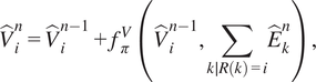 $$ {\hat{V}}_i^n={\hat{V}}_i^{n-1}+{f}_{\pi}^V\left({\hat{V}}_i^{n-1},\sum \limits_{k\mid R(k)=i}{\hat{E}}_k^n\right), $$
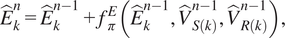 $$ {\hat{E}}_k^n={\hat{E}}_k^{n-1}+{f}_{\pi}^E\left({\hat{E}}_k^{n-1},{\hat{V}}_{S(k)}^{n-1},{\hat{V}}_{R(k)}^{n-1}\right), $$
where each edge
 $ {e}_k $
is assumed to point from node
$ {e}_k $
is assumed to point from node
 $ {v}_{S(k)} $
to node
$ {v}_{S(k)} $
to node
 $ {v}_{R(k)} $
. The same message-passing operations are learned and applied everywhere in the graph. The decoder
$ {v}_{R(k)} $
. The same message-passing operations are learned and applied everywhere in the graph. The decoder
 $ {f}_{\delta } $
is a multilayer perceptron that operates on node features only. The decoded output of the model at node
$ {f}_{\delta } $
is a multilayer perceptron that operates on node features only. The decoded output of the model at node
 $ {v}_i $
is given by
$ {v}_i $
is given by
 $ {Y}_i={f}_{\delta}\left({\hat{V}}_i^N\right) $
. Following Dupuy et al. (Reference Dupuy, Odier, Lapeyre and Papadogiannis2023b), the size of the latent space is
$ {Y}_i={f}_{\delta}\left({\hat{V}}_i^N\right) $
. Following Dupuy et al. (Reference Dupuy, Odier, Lapeyre and Papadogiannis2023b), the size of the latent space is
 $ {d}_L=128 $
at both nodes and edges and the number of processing steps is
$ {d}_L=128 $
at both nodes and edges and the number of processing steps is
 $ N=4 $
in the present study. This value implies that edge and node features that are within a distance up to
$ N=4 $
in the present study. This value implies that edge and node features that are within a distance up to
 $ N=4 $
neighbors away from a given target wall node will influence the prediction. This value was found to be sufficient to discriminate non-equilibrium regions in Dupuy et al. (Reference Dupuy, Odier, Lapeyre and Papadogiannis2023b). The multilayer perceptrons
$ N=4 $
neighbors away from a given target wall node will influence the prediction. This value was found to be sufficient to discriminate non-equilibrium regions in Dupuy et al. (Reference Dupuy, Odier, Lapeyre and Papadogiannis2023b). The multilayer perceptrons
 $ {f}_{\varepsilon}^V $
,
$ {f}_{\varepsilon}^V $
,
 $ {f}_{\varepsilon}^E $
,
$ {f}_{\varepsilon}^E $
,
 $ {f}_{\pi}^V $
, and
$ {f}_{\pi}^V $
, and
 $ {f}_{\pi}^E $
are composed of
$ {f}_{\pi}^E $
are composed of
 $ {n}_{\mathrm{\ell}}=2 $
layers while the multilayer perceptron
$ {n}_{\mathrm{\ell}}=2 $
layers while the multilayer perceptron
 $ {f}_{\delta}^V $
is composed of
$ {f}_{\delta}^V $
is composed of
 $ {n}_{\mathrm{\ell}}+1 $
hidden layers. Each layer is composed of
$ {n}_{\mathrm{\ell}}+1 $
hidden layers. Each layer is composed of
 $ {d}_L $
neural units with a rectified linear unit
$ {d}_L $
neural units with a rectified linear unit
 $ \sigma (x)=\max \left(0,x\right) $
as activation function and is followed by layer normalization (Ba et al., Reference Ba, Kiros and Hinton2016), except for the last layer of the multilayer perceptron
$ \sigma (x)=\max \left(0,x\right) $
as activation function and is followed by layer normalization (Ba et al., Reference Ba, Kiros and Hinton2016), except for the last layer of the multilayer perceptron
 $ {f}_{\delta}^V $
which is linear. The weights of the multilayer perceptrons are learned using the Adam optimizer (Kingma and Ba, Reference Kingma and Ba2015) with a base learning rate of 0.001.
$ {f}_{\delta}^V $
which is linear. The weights of the multilayer perceptrons are learned using the Adam optimizer (Kingma and Ba, Reference Kingma and Ba2015) with a base learning rate of 0.001.
Two graph neural network wall models are trained in order to model the wall shear stress and the wall conductive heat flux respectively. In both cases, the following features are included in the input
 $ \mathbf{X} $
of the model:
$ \mathbf{X} $
of the model:
-
• At the nodes: the three components of the velocity vector, the density, the dynamic viscosity, and a target boundary mask
$ \chi $
equal to 1 on the target wall nodes
$ \mathfrak{W} $
and 0 otherwise; -
• At the edges: the three components of the edge displacement vector, and the length of the edge.


To provide the geometric information of the mesh to the model, we preferred to give the displacement vector of the edges, instead of the node coordinates, because it implies that the input graph will be the same if the geometry is translated, ensuring the translational invariance of the prediction. The angle or distance to the wall is not given to the model as an input. However, it is possible for the model to reconstruct the distance to the wall of an information at a given node, based on the displacement vectors of the various edges connecting the point to the wall. The rationale is to alleviate the need to manually define robust geometrical metrics that can adapt to any complex geometry, and instead opts to let the network learn the optimal way to extract the necessary information itself. The loss function is the mean squared error (MSE) between the output of the model and the reference wall shear stress or wall conductive heat flux, that is either
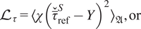 $$ {\mathrm{\mathcal{L}}}_{\tau }={\left\langle \chi {\left({\overset{\check{}}{\overline{\tau}}}_{\mathrm{ref}}^S-Y\right)}^2\right\rangle}_{\mathfrak{A}},\mathrm{or} $$
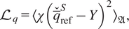 $$ {\mathrm{\mathcal{L}}}_q={\left\langle \chi {\left({\overset{\check{}}{\overline{q}}}_{\mathrm{ref}}^S-Y\right)}^2\right\rangle}_{\mathfrak{A}}, $$
with
 $ {\left\langle \cdot \right\rangle}_{\mathfrak{A}} $
an average across graph nodes and samples. All the input and reference output variables are scaled and/or augmented as described in Section 3.2. To minimize the loss, the learned function has to be resilient to a change of the mesh. Indeed, the training databases prepared in Section 2.1 aggregates various meshes with different resolutions for a given simulation, and the different geometries associated with the different configurations. Furthermore, there are variations present within a given tetrahedral mesh as well. An accurate prediction of the wall shear stress or wall conductive heat flux thus entails being robust to mesh modifications. This will be confirmed in a priori tests.
$ {\left\langle \cdot \right\rangle}_{\mathfrak{A}} $
an average across graph nodes and samples. All the input and reference output variables are scaled and/or augmented as described in Section 3.2. To minimize the loss, the learned function has to be resilient to a change of the mesh. Indeed, the training databases prepared in Section 2.1 aggregates various meshes with different resolutions for a given simulation, and the different geometries associated with the different configurations. Furthermore, there are variations present within a given tetrahedral mesh as well. An accurate prediction of the wall shear stress or wall conductive heat flux thus entails being robust to mesh modifications. This will be confirmed in a priori tests.
5. A priori results
An a priori assessment of the graph neural network wall models is first performed, using filtered wall-resolved simulations to assess the machine-learning procedure. Two machine-learning models are investigated:
-
• a graph neural network wall model, hereafter referred to as the Full GNN model, that is trained on the incompressible channel flows (CF1, CF2), the three-dimensional diffuser (3DD), the NACA 65-009 blade cascade at an incidence angle of 4° (N65) and the cooled/heated channel flows (AC1, AC2, SC1, SC2); and
-
• a graph neural network wall model, hereafter referred to as the ACSC GNN model, that is trained only on the asymmetrically cooled/heated and symmetrically cooled channel flows (AC1, AC2, SC1, SC2).
For each simulation in the training simulation, a subset of the data is isolated for validation purpose. The simulations that are not included in the training or validation dataset are referred to as test simulations. For the Full GNN model, the test simulations are the BFS and APG simulations in the incompressible isothermal case, and the L89 simulation in the compressible anisothermal case. For the ACSC GNN model, the test simulations are all the incompressible isothermal simulations, and the L89 simulation in the compressible anisothermal case.
The coefficient of determination between the reference wall shear stress or wall conductive heat flux and the model prediction
 $ Y $
gives an overview of the model performance (Table 3). It is defined for the wall shear stress model as
$ Y $
gives an overview of the model performance (Table 3). It is defined for the wall shear stress model as
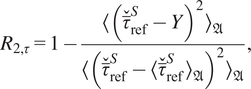 $$ {R}_{2,\tau }=1-\frac{{\left\langle {\left({\overset{\check{}}{\overline{\tau}}}_{\mathrm{ref}}^S-Y\right)}^2\right\rangle}_{\mathfrak{A}}}{{\left\langle {\left({\overset{\check{}}{\overline{\tau}}}_{\mathrm{ref}}^S-{\left\langle {\overset{\check{}}{\overline{\tau}}}_{\mathrm{ref}}^S\right\rangle}_{\mathfrak{A}}\right)}^2\right\rangle}_{\mathfrak{A}}}, $$
and for the conductive heat flux model as
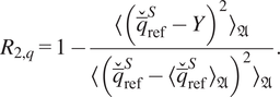 $$ {R}_{2,q}=1-\frac{{\left\langle {\left({\overset{\check{}}{\overline{q}}}_{\mathrm{ref}}^S-Y\right)}^2\right\rangle}_{\mathfrak{A}}}{{\left\langle {\left({\overset{\check{}}{\overline{q}}}_{\mathrm{ref}}^S-{\left\langle {\overset{\check{}}{\overline{q}}}_{\mathrm{ref}}^S\right\rangle}_{\mathfrak{A}}\right)}^2\right\rangle}_{\mathfrak{A}}}. $$
Table 3. Coefficient of determination between the prediction of the graph neural network wall model and the reference for the wall shear stress prediction and the wall heat flux prediction in each dataset
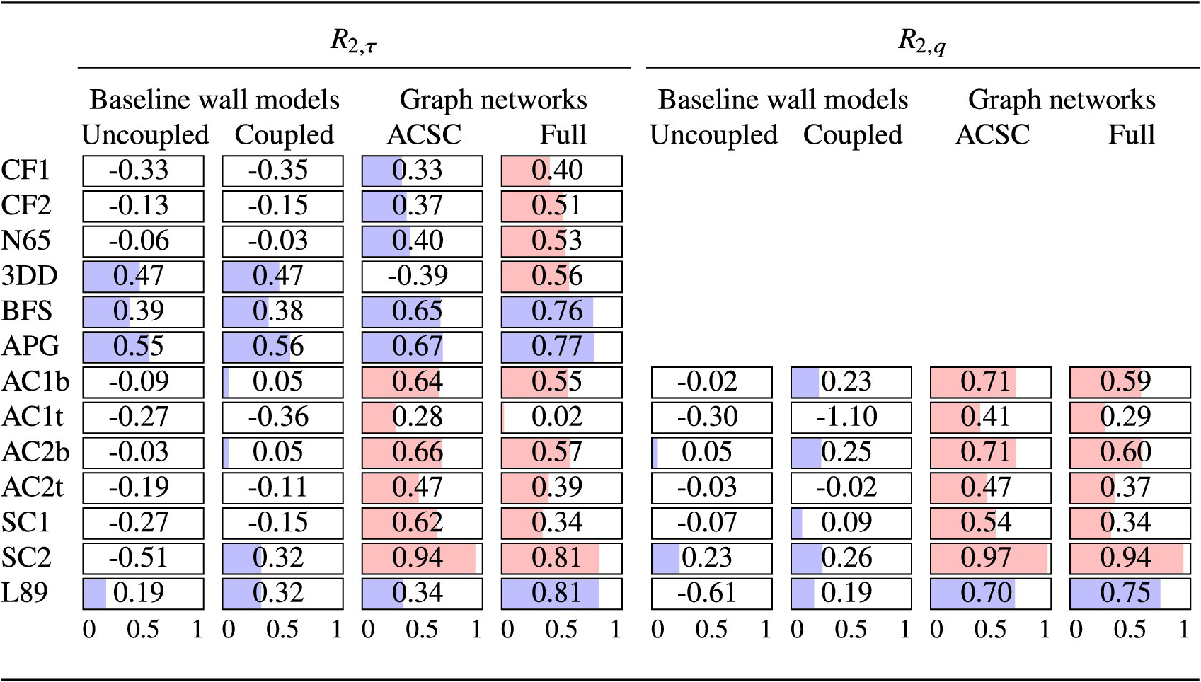
Note. The datasets AC1 and AC2 are split respectively into AC1b and AC2b, corresponding to the bottom (cold) wall, and AC1t and AC2t, corresponding to the top (hot) wall. The cells are tinted in red if the simulation was included in the training or validation dataset of the corresponding model and are tinted in blue otherwise, that is for test simulations. It should be noted that the value of the coefficient of determination associated with two different simulations cannot be directly compared, as an identical value of
 $ {R}_2 $
may provide a satisfactory performance for a given simulation but not for another.
$ {R}_2 $
may provide a satisfactory performance for a given simulation but not for another.
It should be emphasized that the coefficient of determination is an imperfect measure of the model performance, as it also depends on the underlying distribution of the data and cannot easily be compared between different datasets. For instance, if two datasets are artificially combined to form an unique dataset, the resulting coefficient of determination can be larger than the coefficient of determination associated with each dataset, taken separately. Hence, an identical value of
 $ {R}_2 $
may provide a satisfactory performance for a given simulation but not for another. However, the values of determination coefficient can readily be compared across different models for a given simulation, since the dataset is fixed. Based on the coefficient of determination, the validation performance of the ACSC model is satisfactory, as the model is significantly more accurate than the baseline algebraic models in the training simulations AC1, AC2, SC1, and SC2. Although no incompressible isothermal simulation was included in the training dataset, the ACSC model generalizes well to an incompressible isothermal channel flow (case CF1 or CF2). This is confirmed by the
$ {R}_2 $
may provide a satisfactory performance for a given simulation but not for another. However, the values of determination coefficient can readily be compared across different models for a given simulation, since the dataset is fixed. Based on the coefficient of determination, the validation performance of the ACSC model is satisfactory, as the model is significantly more accurate than the baseline algebraic models in the training simulations AC1, AC2, SC1, and SC2. Although no incompressible isothermal simulation was included in the training dataset, the ACSC model generalizes well to an incompressible isothermal channel flow (case CF1 or CF2). This is confirmed by the
 $ {u}^{+}\left({y}^{+}\right) $
scatter plots in Figure 3a,b, in which it may be seen that the predictions of the ACSC model are scatter around Reichardt’s law in the incompressible isothermal channels. Reichardt’s profile in Figure 3 is given by the following analytical expression of the incompressible law of the wall (Reichardt, Reference Reichardt1951):
$ {u}^{+}\left({y}^{+}\right) $
scatter plots in Figure 3a,b, in which it may be seen that the predictions of the ACSC model are scatter around Reichardt’s law in the incompressible isothermal channels. Reichardt’s profile in Figure 3 is given by the following analytical expression of the incompressible law of the wall (Reichardt, Reference Reichardt1951):
 $$ {u}^{+}\left({y}^{+}\right)=\frac{1}{\kappa}\log \left(1+\kappa {y}^{+}\right)+7.8\left[1-\exp \left(\frac{-{y}^{+}}{11}\right)-\frac{y^{+}}{11}\exp \left(\frac{-{y}^{+}}{3}\right)\right], $$
with
 $ \kappa =0.41 $
the von Kármán constant. In the cooled/heated channels, the model prediction deviates from Reichardt’s law due to the effect of the large temperature variations on the velocity profile, which is consistent with the behavior of the reference filtered data (Figure 3g–j). Similarly, the reference mean temperature profile may in the cooled/heated channels deviate from Kader’s law (Kader, Reference Kader1981)
$ \kappa =0.41 $
the von Kármán constant. In the cooled/heated channels, the model prediction deviates from Reichardt’s law due to the effect of the large temperature variations on the velocity profile, which is consistent with the behavior of the reference filtered data (Figure 3g–j). Similarly, the reference mean temperature profile may in the cooled/heated channels deviate from Kader’s law (Kader, Reference Kader1981)
 $$ {T}^{+}\left({y}^{+}\right)=\mathit{\Pr}\hskip0.1em {y}^{+}\exp \left(-\frac{0.01{\left({Pry}^{+}\right)}^4}{1+5{\mathit{\Pr}}^3{y}^{+}}\right)+\left[2.12\log \left(1+{y}^{+}\right)+{C}_T\right]\exp \left(-\frac{1+5{\mathit{\Pr}}^3{y}^{+}}{0.01{\left({Pry}^{+}\right)}^4}\right), $$
where
 $ {C}_T $
is defined in equation (19), due to the effect of the coupling between velocity and temperature. This is well reproduced by the ACSC model in the simulations AC1, AC2, SC1, and SC2 (Figure 4a–d). This is confirmed by the scatter plots in Figure 6a–d, which show a good overall agreement between the model prediction and the reference value in those simulations. However, the ACSC model may only operate on channel flows and lead to a poor performance in non-equilibrium configurations for which it has not been trained. For instance, the mean prediction of the ACSC model in the incompressible isothermal test case BFS does not reproduce the spatial variations found in the reference filtered data (Figure 7a). Nevertheless, the predictions of the ACSC model in the non-equilibrium simulations BFS, APG, and L89 are at least as accurate as the algebraic coupled or uncoupled wall models, which are also intended for equilibrium flow configurations. In particular, the mean wall shear stress prediction of the ACSC model is more accurate than that of the algebraic models throughout the domain in the APG simulation (Figure 7b). Moreover, the mean conductive heat flux prediction of the ACSC model in the L89 simulation is significantly more accurate than that of the algebraic models on both the pressure side (
$ {C}_T $
is defined in equation (19), due to the effect of the coupling between velocity and temperature. This is well reproduced by the ACSC model in the simulations AC1, AC2, SC1, and SC2 (Figure 4a–d). This is confirmed by the scatter plots in Figure 6a–d, which show a good overall agreement between the model prediction and the reference value in those simulations. However, the ACSC model may only operate on channel flows and lead to a poor performance in non-equilibrium configurations for which it has not been trained. For instance, the mean prediction of the ACSC model in the incompressible isothermal test case BFS does not reproduce the spatial variations found in the reference filtered data (Figure 7a). Nevertheless, the predictions of the ACSC model in the non-equilibrium simulations BFS, APG, and L89 are at least as accurate as the algebraic coupled or uncoupled wall models, which are also intended for equilibrium flow configurations. In particular, the mean wall shear stress prediction of the ACSC model is more accurate than that of the algebraic models throughout the domain in the APG simulation (Figure 7b). Moreover, the mean conductive heat flux prediction of the ACSC model in the L89 simulation is significantly more accurate than that of the algebraic models on both the pressure side (
 $ {s}_1<0 $
) and the suction side (
$ {s}_1<0 $
) and the suction side (
 $ {s}_1>0 $
) of the blade, although the mean wall shear stress prediction is not more accurate (Figure 7c). This shows that the graph neural network wall model can generalize to non-equilibrium flows at least as well as the two algebraic models investigated, but to a very limited extent as only cooled/heated channel flows were included in the training dataset for the ACSC model. To improve the capability of the model, it is necessary to include a more varied physics in the training dataset.
$ {s}_1>0 $
) of the blade, although the mean wall shear stress prediction is not more accurate (Figure 7c). This shows that the graph neural network wall model can generalize to non-equilibrium flows at least as well as the two algebraic models investigated, but to a very limited extent as only cooled/heated channel flows were included in the training dataset for the ACSC model. To improve the capability of the model, it is necessary to include a more varied physics in the training dataset.
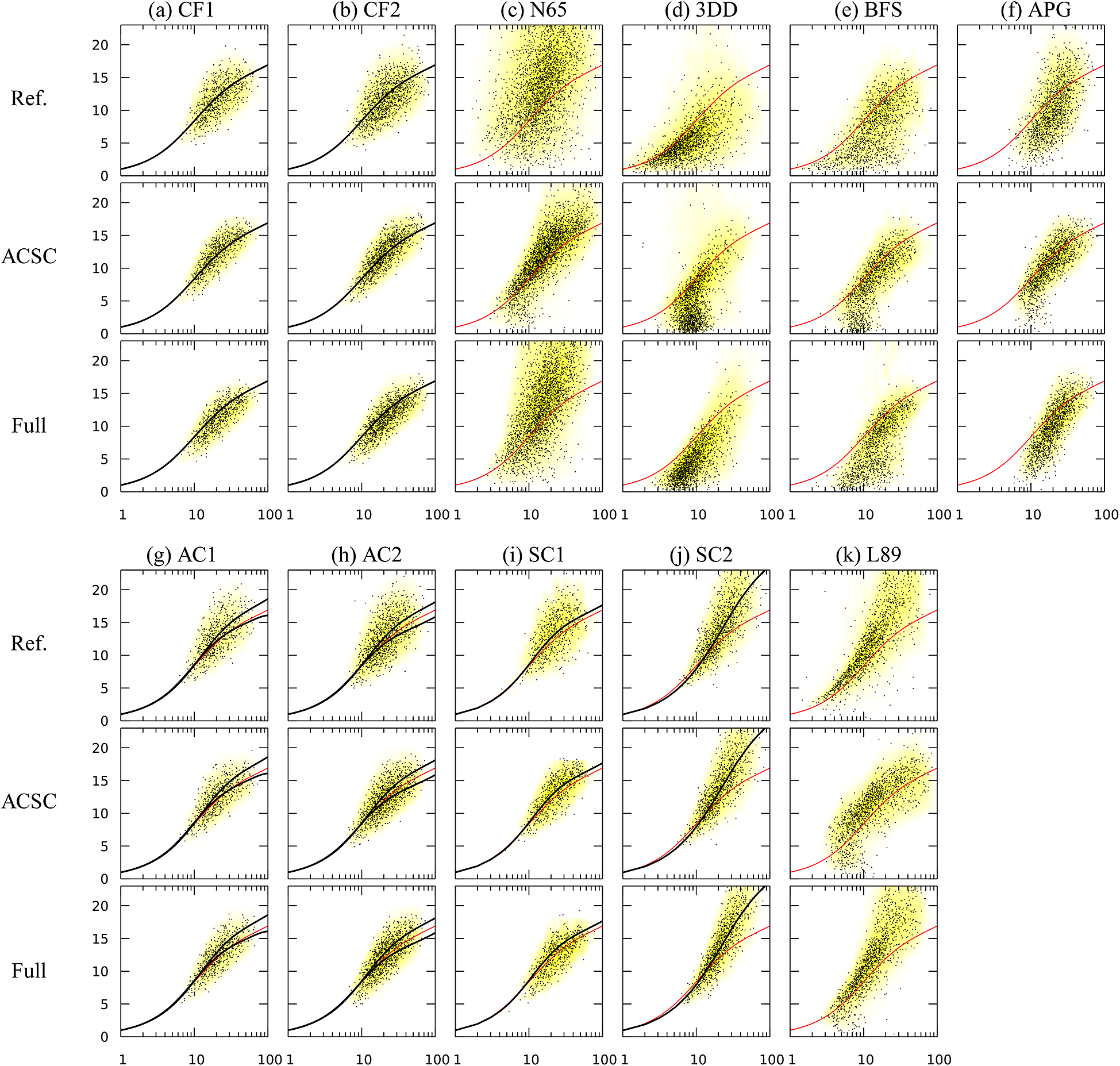
Figure 3.
Scaled wall-tangential velocity
 $ {u}^{+} $
as a function of the scaled distance to the wall
$ {u}^{+} $
as a function of the scaled distance to the wall
 $ {y}^{+} $
in each dataset using the local reference wall shear stress (top), the prediction of the ACSC model (center), and the prediction of the Full model (bottom) to compute the wall unit scaling (
$ {y}^{+} $
in each dataset using the local reference wall shear stress (top), the prediction of the ACSC model (center), and the prediction of the Full model (bottom) to compute the wall unit scaling (
 $ {}^{+} $
). The red line is Reichardt’s law, given by equation (31). The black line is the mean profile of the reference simulation. It is given only when applicable that is in spatially homogeneous simulations. Two mean profiles are given in the case AC1 and AC2, one for the top (hot) wall and one for the bottom (cold) wall.
$ {}^{+} $
). The red line is Reichardt’s law, given by equation (31). The black line is the mean profile of the reference simulation. It is given only when applicable that is in spatially homogeneous simulations. Two mean profiles are given in the case AC1 and AC2, one for the top (hot) wall and one for the bottom (cold) wall.
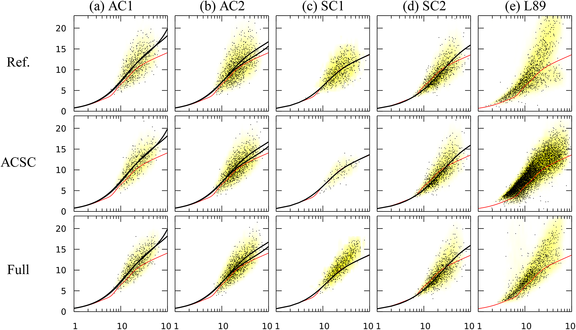
Figure 4.
Scaled temperature
 $ {T}^{+} $
as a function of the scaled distance to the wall
$ {T}^{+} $
as a function of the scaled distance to the wall
 $ {y}^{+} $
in each dataset using the local reference wall shear stress (top), the prediction of the ACSC model (center), and the prediction of the Full model (bottom) to compute the wall unit scaling (
$ {y}^{+} $
in each dataset using the local reference wall shear stress (top), the prediction of the ACSC model (center), and the prediction of the Full model (bottom) to compute the wall unit scaling (
 $ {}^{+} $
). The red line is Kader’s law, given by equation ((32). The black line is the mean profile of the reference simulation. It is given only when applicable that is in spatially homogeneous simulations. Two mean profiles are given in the case AC1 and AC2, one for the top (hot) wall and one for the bottom (cold) wall.
$ {}^{+} $
). The red line is Kader’s law, given by equation ((32). The black line is the mean profile of the reference simulation. It is given only when applicable that is in spatially homogeneous simulations. Two mean profiles are given in the case AC1 and AC2, one for the top (hot) wall and one for the bottom (cold) wall.
The Full model, trained on a combination of cooled/heated channels and equilibrium and non-equilibrium incompressible isothermal flows, is able to handle a wider range of flow configurations. The coefficients of determination of the Full model on the cooled/heated channels are slightly lower than those of the ACSC model, fitted specifically to these simulations. The validation performance of the Full model in the training simulations AC1, AC2, SC1, and SC2 remains satisfactory. Indeed, the prediction of the model is scattered around the mean velocity profile (Figure 3g,h,j) and the mean temperature profile (Figure 4a,b,d) of the simulations AC1, AC2, and SC2. In the simulation SC1, which features a low coupling between velocity and temperature, the Full model deviates too much from Kader’s law (32) in the
 $ {T}^{+}\left({y}^{+}\right) $
scatter plot. The Full model also provides relevant predictions in the incompressible isothermal channels CF1 and CF2 (Figure 3a,b). Finally, the Full model can accurately predict the wall shear stress in non-equilibrium flow configurations. In particular, the behavior in the
$ {T}^{+}\left({y}^{+}\right) $
scatter plot. The Full model also provides relevant predictions in the incompressible isothermal channels CF1 and CF2 (Figure 3a,b). Finally, the Full model can accurately predict the wall shear stress in non-equilibrium flow configurations. In particular, the behavior in the
 $ {u}^{+}\left({y}^{+}\right) $
scatter plots of the training simulations N65 and 3DD (Figure 3c,d) and the test simulations BFS, APG, and L89 (Figure 3e,f,k) is qualitatively well reproduced by the Full model, although a non-negligible amount of variance is not captured. Figures 5c–e,g,k and 6e show that the agreement between the model prediction and the reference value is greater in these non-homogeneous configurations than either the algebraic coupled or uncoupled wall models or the ACSC model. Figure 7 demonstrates that, overall, the Full model captures well the spatial variations of mean wall shear stress in the test simulations BFS and APG and the spatial variations of both wall shear stress and conductive heat flux in the simulation L89. In the three cases, the Full model provides a clear improvement compared to both the algebraic wall models and the ACSC model. Overall, these a priori results suggest that the Full model can, within a reasonable range of flow configurations, take into account both non-equilibrium effects, such as flow separation, and the effect of large temperature variations on the wall shear stress and conductive heat flux prediction. The performance of the trained model on the test simulations, for geometries and meshes not seen during training, also proves the model is robust to variations of the mesh.
$ {u}^{+}\left({y}^{+}\right) $
scatter plots of the training simulations N65 and 3DD (Figure 3c,d) and the test simulations BFS, APG, and L89 (Figure 3e,f,k) is qualitatively well reproduced by the Full model, although a non-negligible amount of variance is not captured. Figures 5c–e,g,k and 6e show that the agreement between the model prediction and the reference value is greater in these non-homogeneous configurations than either the algebraic coupled or uncoupled wall models or the ACSC model. Figure 7 demonstrates that, overall, the Full model captures well the spatial variations of mean wall shear stress in the test simulations BFS and APG and the spatial variations of both wall shear stress and conductive heat flux in the simulation L89. In the three cases, the Full model provides a clear improvement compared to both the algebraic wall models and the ACSC model. Overall, these a priori results suggest that the Full model can, within a reasonable range of flow configurations, take into account both non-equilibrium effects, such as flow separation, and the effect of large temperature variations on the wall shear stress and conductive heat flux prediction. The performance of the trained model on the test simulations, for geometries and meshes not seen during training, also proves the model is robust to variations of the mesh.
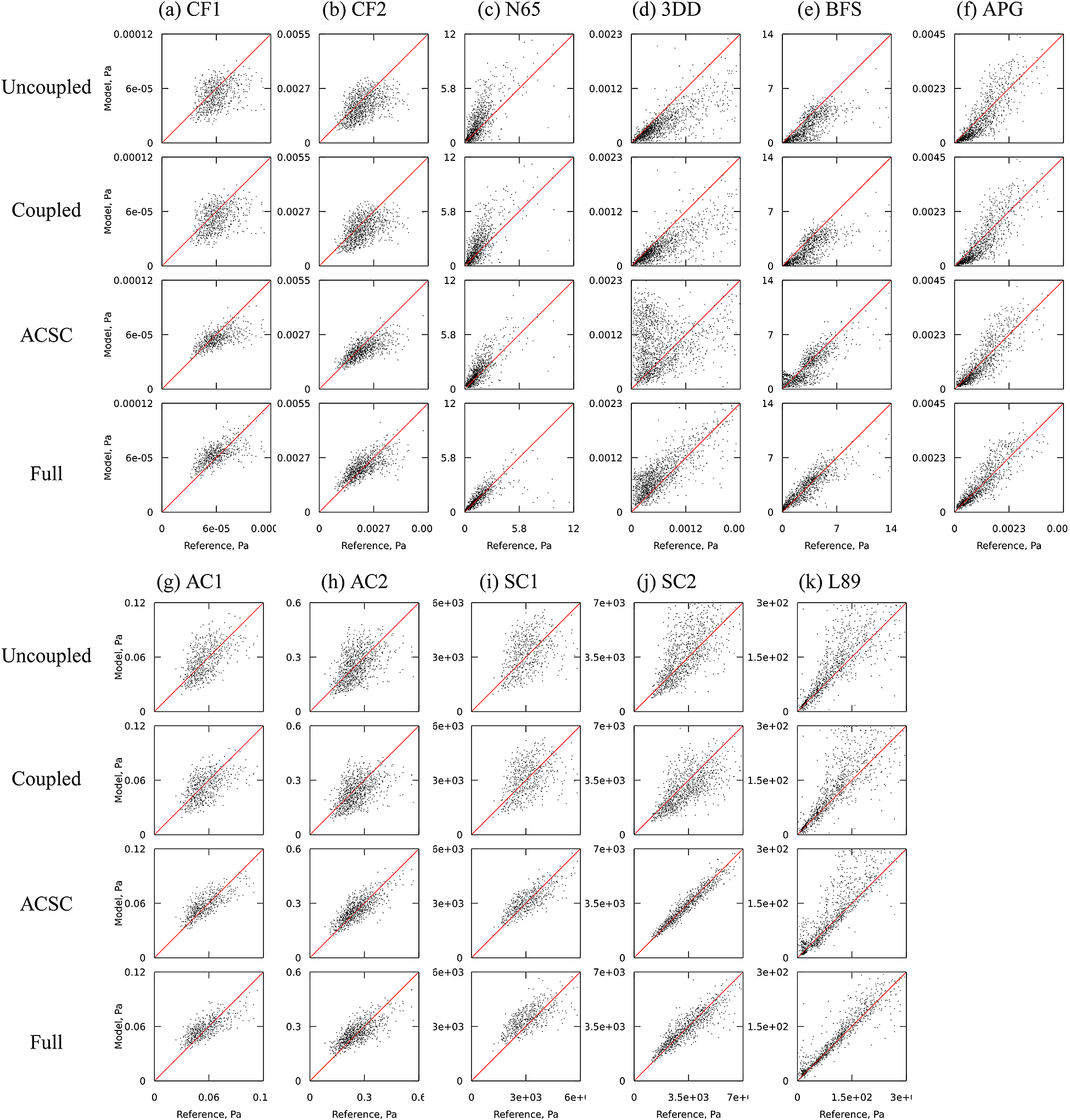
Figure 5. Scatter plot between the target wall shear stress and the prediction of the uncoupled algebraic wall model, the coupled algebraic wall model, the ACSC model, and the Full model. The red line is identity.
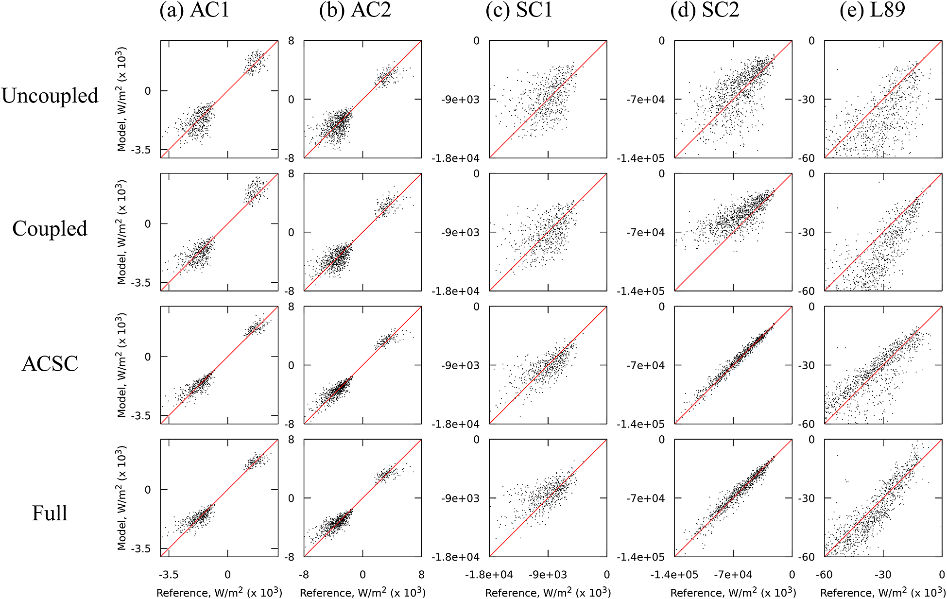
Figure 6. Scatter plot between the target wall conductive heat flux and the prediction of the uncoupled algebraic wall model, the coupled algebraic wall model, the ACSC model, and the Full model. The red line is identity.
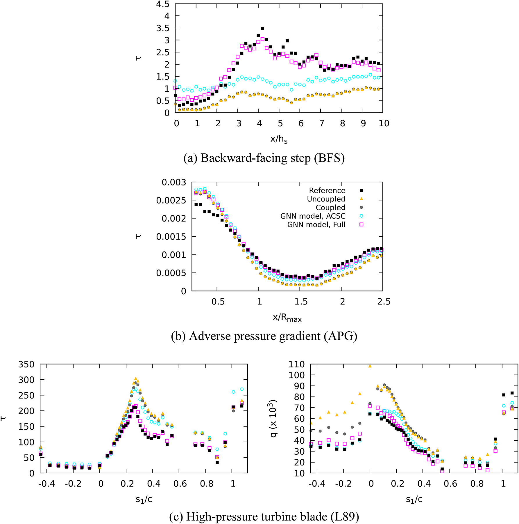
Figure 7.
Average prediction of the baseline wall models and the graph neural network wall models in different test cases. The average is performed in both time and spanwise directions in the BFS simulation, the APG simulation, and the L89 simulation. Both
 $ \tau $
and
$ \tau $
and
 $ q $
are given in dimensional units, namely respectively Pa and W/m
2.
$ q $
are given in dimensional units, namely respectively Pa and W/m
2.
6. A posteriori tests
The graph-based wall modeling approach has been assessed a posteriori in several configurations: two symmetrically cooled channel flows (SC2 and SC3) and a cooled high-pressure turbine blade (L89). The SC2 case aims to validate the ability of the graph neural network wall model to generalize from a priori tests to a posteriori tests, as this is not trivial in LESs particularly for machine-learning models (Sagaut, Reference Sagaut2006). The SC3 simulation aims to confirm the ability of the graph neural network wall model to generalize for a different fully developed channel flow not seen during training. The L89 case aims to demonstrate the ability of the graph neural network wall model to generalize to a complex test configuration that was not included in the training or validation dataset, and a challenging physics that strongly departs from asumptions of a fully developed equilibrium boundary layer.
6.1. Numerical method
In all simulations, the flow is modeled as a continuous medium in local thermodynamic equilibrium using the compressible LES equations and the ideal gas law. These equations may be expressed as follows:
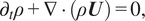 $$ {\partial}_t\rho +\nabla \cdot \left(\rho \boldsymbol{U}\right)=0, $$
 $$ {\partial}_t\left(\rho \boldsymbol{U}\right)+\nabla \cdot \left(\rho \boldsymbol{U}\otimes \boldsymbol{U}\right)=-\nabla P+\nabla \cdot \mathtt{S}, $$
 $$ {\partial}_t\left(\rho E\right)+\nabla \cdot \left(\rho \boldsymbol{U}H\right)=-\nabla \cdot \boldsymbol{Q}-\nabla \cdot \left(\boldsymbol{U}P\right)+\nabla \cdot \left(\boldsymbol{U}\cdot \mathtt{S}\right), $$
 $$ P= r\rho T, $$
where
 $ \rho $
is the density of the fluid,
$ \rho $
is the density of the fluid,
 $ t $
is the time,
$ t $
is the time,
 $ \boldsymbol{U} $
is the velocity,
$ \boldsymbol{U} $
is the velocity,
 $ \boldsymbol{x} $
is the Cartesian coordinate,
$ \boldsymbol{x} $
is the Cartesian coordinate,
 $ P $
is the pressure,
$ P $
is the pressure,
 $ \boldsymbol{Q} $
is the conductive heat flux,
$ \boldsymbol{Q} $
is the conductive heat flux,
 $ E $
is the total energy per unit mass,
$ E $
is the total energy per unit mass,
 $ H=E+P/\rho $
is the total enthalpy per unit mass, and
$ H=E+P/\rho $
is the total enthalpy per unit mass, and
 $ r $
is the specific ideal gas constant. The temperature is computed using tabulated data from Stull and Prophet (Reference Stull and Prophet1971) based on the internal energy
$ r $
is the specific ideal gas constant. The temperature is computed using tabulated data from Stull and Prophet (Reference Stull and Prophet1971) based on the internal energy
 $ e=E-\frac{1}{2}{U}_i{U}_i $
. No external body forces or volumetric heat sources are taken into account. The viscous stress tensor and conductive heat flux are computed assuming a Newtonian fluid under Stokes’ hypothesis and Fourier’s law, while subgrid-scale stresses are modeled using an eddy-viscosity model. The stress tensor
$ e=E-\frac{1}{2}{U}_i{U}_i $
. No external body forces or volumetric heat sources are taken into account. The viscous stress tensor and conductive heat flux are computed assuming a Newtonian fluid under Stokes’ hypothesis and Fourier’s law, while subgrid-scale stresses are modeled using an eddy-viscosity model. The stress tensor
 $ \Sigma $
is given by:
$ \Sigma $
is given by:
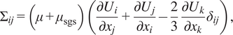 $$ {\Sigma}_{ij}=\left(\mu +{\mu}_{\mathrm{sgs}}\right)\left(\frac{\partial {U}_i}{\partial {x}_j}+\frac{\partial {U}_j}{\partial {x}_i}-\frac{2}{3}\frac{\partial {U}_k}{\partial {x}_k}{\delta}_{ij}\right), $$
where
 $ \mu $
is the dynamic viscosity of the fluid,
$ \mu $
is the dynamic viscosity of the fluid,
 $ {\mu}_{\mathrm{sgs}} $
the subgrid-scale viscosity, and
$ {\mu}_{\mathrm{sgs}} $
the subgrid-scale viscosity, and
 $ {\delta}_{ij} $
denotes the Kronecker delta. The conductive heat flux is computed assuming Fourier’s law and an eddy-diffusivity subgrid-scale contribution:
$ {\delta}_{ij} $
denotes the Kronecker delta. The conductive heat flux is computed assuming Fourier’s law and an eddy-diffusivity subgrid-scale contribution:
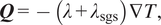 $$ \boldsymbol{Q}=-\left(\lambda +{\lambda}_{\mathrm{sgs}}\right)\nabla T, $$
where
 $ T $
is the fluid temperature and
$ T $
is the fluid temperature and
 $ \lambda $
the thermal conductivity of the fluid, computed using a constant Prandtl number assumption. The subgrid-scale conductivity
$ \lambda $
the thermal conductivity of the fluid, computed using a constant Prandtl number assumption. The subgrid-scale conductivity
 $ {\lambda}_{\mathrm{sgs}}={C}_p{\mu}_{\mathrm{sgs}}/{\mathit{\Pr}}_{\mathrm{sgs}} $
is computed assuming a constant subgrid-scale Prandtl number
$ {\lambda}_{\mathrm{sgs}}={C}_p{\mu}_{\mathrm{sgs}}/{\mathit{\Pr}}_{\mathrm{sgs}} $
is computed assuming a constant subgrid-scale Prandtl number
 $ {\mathit{\Pr}}_{\mathrm{sgs}} $
. The isobaric heat capacity
$ {\mathit{\Pr}}_{\mathrm{sgs}} $
. The isobaric heat capacity
 $ {C}_p $
is computed from tabulated data (Stull and Prophet, Reference Stull and Prophet1971).
$ {C}_p $
is computed from tabulated data (Stull and Prophet, Reference Stull and Prophet1971).
The numerical simulations are performed by coupling the numerical resolution of equations (33)–(36) via the compressible, unstructured, massively parallel flow solver AVBP (Schönfeld and Rudgyard, Reference Schönfeld and Rudgyard1999), to the graph neural network wall model inference. The coupling, implemented via a message passing interface (MPI), is described in Dupuy et al. (Reference Dupuy, Odier, Lapeyre and Papadogiannis2023b). At each time step, data is extracted from the LES fields to create near-wall graphs and sent to the graph neural network for inference. The inference is executed exclusively on graphics processing units (GPUs), concurrently to parts of the LES schemes ran on CPUs. The calculation is distributed across multiple GPUs using a specific GPU partitioning that is separate from the CPU partitioning. To make sure that the model prediction is not influenced by the partitioning, the GPU partitions are overlapped by the number of message-passing steps
 $ N $
of the model. This overlap ensures that each partition includes the receptive field required for the prediction of the wall shear stress and wall heat flux. The predictions are then sent back to the main flow solver to set the boundary conditions in the momentum and energy transport equations.
$ N $
of the model. This overlap ensures that each partition includes the receptive field required for the prediction of the wall shear stress and wall heat flux. The predictions are then sent back to the main flow solver to set the boundary conditions in the momentum and energy transport equations.
6.2. Symmetrically cooled channel flows
This section addresses the wall-modeled LES of symmetrically cooled channel flows. We first consider the simulation SC2, included in the training database. The operating conditions of the wall-modeled simulations are the same as in the wall-resolved simulation (Appendix A), namely, the temperature ratio between the bulk flow and the walls is 3 and the friction Reynolds number is
 $ {\mathit{\operatorname{Re}}}_{\tau }=1150 $
. In the wall-modeled LESs, the size of the domain is
$ {\mathit{\operatorname{Re}}}_{\tau }=1150 $
. In the wall-modeled LESs, the size of the domain is
 $ 14h\times 2h\times 5.2h $
, with
$ 14h\times 2h\times 5.2h $
, with
 $ h $
the half-height. The WMLES mesh contains 8 million tetrahedral cells. The average height of the first point off the wall, in wall units, is
$ h $
the half-height. The WMLES mesh contains 8 million tetrahedral cells. The average height of the first point off the wall, in wall units, is
 $ {y}^{+}=40 $
. As in the wall-resolved simulation, the convective scheme is a two-step Taylor–Galerkin scheme with third-order spatial and temporal accuracy (Colin and Rudgyard, Reference Colin and Rudgyard2000) and the diffusive scheme is a centered second-order scheme. The subgrid-scale viscosity model is the Smagorinsky model (Smagorinsky, Reference Smagorinsky1963).
$ {y}^{+}=40 $
. As in the wall-resolved simulation, the convective scheme is a two-step Taylor–Galerkin scheme with third-order spatial and temporal accuracy (Colin and Rudgyard, Reference Colin and Rudgyard2000) and the diffusive scheme is a centered second-order scheme. The subgrid-scale viscosity model is the Smagorinsky model (Smagorinsky, Reference Smagorinsky1963).
Wall-modeled LESs using the baseline uncoupled and coupled algebraic models, the ACSC and Full graph neural network wall models are compared in Figure 8. Namely, the profiles of mean streamwise velocity, mean temperature, standard deviation of streamwise velocity, and standard deviation of temperature are provided using the classical wall scaling (
 $ + $
). The uncoupled algebraic model leads to a mean temperature profile that is farther from the reference mean temperature profile than the other investigated models, since it neglects the effect of the large temperature variations. The uncoupled algebraic model and the two graph neural network wall models lead to profiles that are close to one another. The profiles obtained using the Full model are slightly closer to the reference wall-resolved profiles of temperature and velocity. With the Full model, the mean temperature profile is very close to the reference profile above
$ + $
). The uncoupled algebraic model leads to a mean temperature profile that is farther from the reference mean temperature profile than the other investigated models, since it neglects the effect of the large temperature variations. The uncoupled algebraic model and the two graph neural network wall models lead to profiles that are close to one another. The profiles obtained using the Full model are slightly closer to the reference wall-resolved profiles of temperature and velocity. With the Full model, the mean temperature profile is very close to the reference profile above
 $ {y}^{+}=200 $
while the slope of the profile is overestimated closer to the wall. The mean velocity profile is shifted upward compared to the reference profile in the logarithmic region. This behavior is alike the logarithmic layer mismatch that is classically obtained in wall-modeled LES, due to numerical and subgrid-modeling errors in the first few grid points (Kawai and Larsson, Reference Kawai and Larsson2012; Larsson et al., Reference Larsson, Kawai, Bodart and Bermejo-Moreno2016; Bose and Park, Reference Bose and Park2018). This is confirmed by the simulation of an incompressible channel in the absence of thermal effects (Appendix B). The magnitude of the peak standard deviation of streamwise velocity is well predicted by all wall-modeled LESs (Figure 8), but its height is overestimated compared to the reference wall-resolved simulation. The peak standard deviation of temperature is also farther from the wall than in the reference, and its magnitude is underestimated by around 10%. Both the standard deviation of streamwise velocity and temperature are overestimated in the bulk of the channel in all wall-modeled LESs. For all turbulence statistics investigated, the profiles obtained with the two graph neural network wall models and with the baseline coupled algebraic model are very similar. To assess the influence of the subgrid-scale model on this conclusion, we performed simulations of the cooled channel SC2 using the Sigma subgrid-scale model (Nicoud et al., Reference Nicoud, Baya Toda, Cabrit, Bose and Lee2011). The simulations with the Sigma model exhibit a more pronounced logarithmic-layer mismatch compared to the simulations with the Smagorinsky model (Figure 9). This is consistent with studies from the literature, which have found that, in wall-modeled simulations, the Smagorinsky model provides a more accurate wall shear stress prediction than the Sigma model in a channel flow (Blanchard et al., Reference Blanchard, Odier, Gicquel, Cuenot and Nicoud2021). The profiles obtained with the Full graph neural network wall model and the baseline coupled algebraic model are similar to the Smagorinsky model. This confirms that, for the simulation of the symmetrically cooled channel flow SC2 included in the training database, the graph neural network wall models can operate in an a posteriori configuration and reach parity performance with a state-of-the-art algebraic model.
$ {y}^{+}=200 $
while the slope of the profile is overestimated closer to the wall. The mean velocity profile is shifted upward compared to the reference profile in the logarithmic region. This behavior is alike the logarithmic layer mismatch that is classically obtained in wall-modeled LES, due to numerical and subgrid-modeling errors in the first few grid points (Kawai and Larsson, Reference Kawai and Larsson2012; Larsson et al., Reference Larsson, Kawai, Bodart and Bermejo-Moreno2016; Bose and Park, Reference Bose and Park2018). This is confirmed by the simulation of an incompressible channel in the absence of thermal effects (Appendix B). The magnitude of the peak standard deviation of streamwise velocity is well predicted by all wall-modeled LESs (Figure 8), but its height is overestimated compared to the reference wall-resolved simulation. The peak standard deviation of temperature is also farther from the wall than in the reference, and its magnitude is underestimated by around 10%. Both the standard deviation of streamwise velocity and temperature are overestimated in the bulk of the channel in all wall-modeled LESs. For all turbulence statistics investigated, the profiles obtained with the two graph neural network wall models and with the baseline coupled algebraic model are very similar. To assess the influence of the subgrid-scale model on this conclusion, we performed simulations of the cooled channel SC2 using the Sigma subgrid-scale model (Nicoud et al., Reference Nicoud, Baya Toda, Cabrit, Bose and Lee2011). The simulations with the Sigma model exhibit a more pronounced logarithmic-layer mismatch compared to the simulations with the Smagorinsky model (Figure 9). This is consistent with studies from the literature, which have found that, in wall-modeled simulations, the Smagorinsky model provides a more accurate wall shear stress prediction than the Sigma model in a channel flow (Blanchard et al., Reference Blanchard, Odier, Gicquel, Cuenot and Nicoud2021). The profiles obtained with the Full graph neural network wall model and the baseline coupled algebraic model are similar to the Smagorinsky model. This confirms that, for the simulation of the symmetrically cooled channel flow SC2 included in the training database, the graph neural network wall models can operate in an a posteriori configuration and reach parity performance with a state-of-the-art algebraic model.
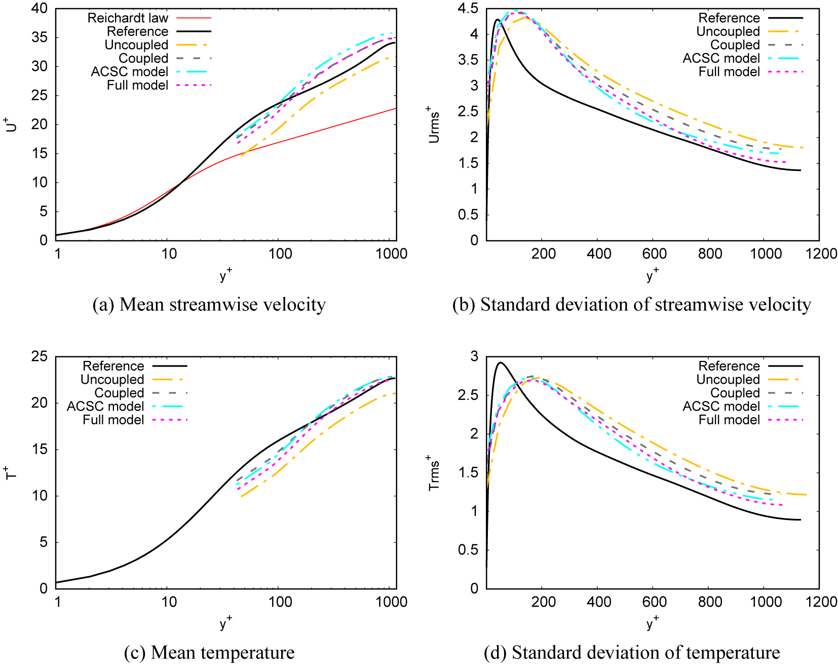
Figure 8. Mean streamwise velocity, standard deviation of streamwise velocity, mean temperature, and standard deviation of temperature in large-eddy simulations of the symmetrically cooled channel flow SC2 with algebraic wall models and graph neural network wall models. The wall-resolved simulation presented in Appendix A is given for comparison.
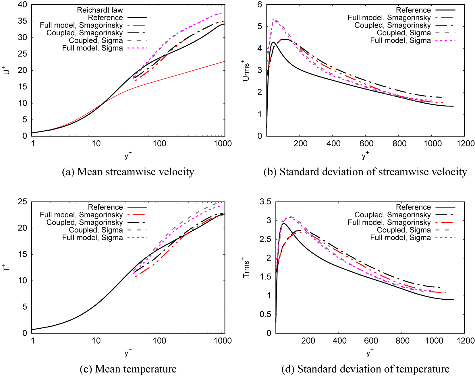
Figure 9. Mean streamwise velocity, standard deviation of streamwise velocity, mean temperature, and standard deviation of temperature in large-eddy simulations of the symmetrically cooled channel flow SC2 with algebraic wall models and graph neural network wall models, using the Smagorinsky and Sigma subgrid-scale models. The wall-resolved simulation presented in Appendix A is given for comparison.
The graph neural network wall models are now assessed for the wall-modeled LES of the symmetrically cooled channel flow SC3, not included in the training database. As described in Appendix A, the flow SC3 is similar to the flow SC2 but uses air as working fluid. In particular, the dynamic viscosity law, the ideal gas specific constant, and the scales of velocity, density, and pressure are modified compared to the case SC2. The mass flow rate is adjusted in order to preserve a similar mean friction Reynolds number to the simulation SC2. The computation domain, the mesh, and the numerical method used in the wall-modeled LESs are identical to those used for the simulation SC2. The numerical results are given in Figure 10. Similar to the SC2 simulation, the uncoupled algebraic model leads to a more inaccurate mean temperature profile than the coupled algebraic model, which is better suited to flows with large temperature variations. The Full model and the coupled algebraic model lead to very similar profiles for all turbulence statistics investigated. The mean velocity profile is as in the SC2 case overestimated in the logarithmic region but, as opposed to the SC2 case, the mean temperature profile is also overestimated in this region. Moreover, the standard deviation of both streamwise velocity and temperature is overestimated in the center of the channel but as in the SC2 simulation its peak magnitude is reasonably well predicted (less than 10% error). The wall-modeled LES with the ACSC model lead to a less accurate mean velocity profile than the simulation with the Full model. Overall, the Full model seems able to generalize to a symmetrically cooled channel flow, even for a different working fluid than seen during training. To provide a more quantitative assessment of the accuracy of the wall models, Table 4 reports the mean wall shear stress and conductive heat flux of each wall-modeled LES. The Full graph neural network wall model is slightly more accurate than the coupled algebraic model for the prediction of the mean wall shear stress in the SC2 and SC3 simulations, but slightly less accurate for the prediction of the wall conductive heat flux in the SC3 simulation.
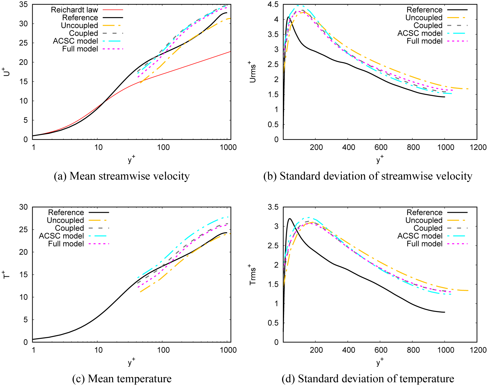
Figure 10. Mean streamwise velocity, standard deviation of streamwise velocity, mean temperature, and standard deviation of temperature in large-eddy simulations of the symmetrically cooled channel flow SC3 with algebraic wall models and graph neural network wall models. The wall-resolved simulation presented in Appendix A is given for comparison.
Table 4.
Mean nondimensionalized wall shear stress
 $ \tau /\left(\rho {u}_c^2\right)={\left({u}_{\tau }/{u}_c\right)}^2 $
, where
$ \tau /\left(\rho {u}_c^2\right)={\left({u}_{\tau }/{u}_c\right)}^2 $
, where
 $ {u}_c $
is the centerline velocity, in large-eddy simulations of a channel flow at the friction Reynolds numbers
$ {u}_c $
is the centerline velocity, in large-eddy simulations of a channel flow at the friction Reynolds numbers
 $ {\mathit{\operatorname{Re}}}_{\tau }=395 $
,
$ {\mathit{\operatorname{Re}}}_{\tau }=395 $
,
 $ {\mathit{\operatorname{Re}}}_{\tau }=950 $
, and
$ {\mathit{\operatorname{Re}}}_{\tau }=950 $
, and
 $ {\mathit{\operatorname{Re}}}_{\tau }=2000 $
with an algebraic wall stress model and a machine-learning wall model
$ {\mathit{\operatorname{Re}}}_{\tau }=2000 $
with an algebraic wall stress model and a machine-learning wall model
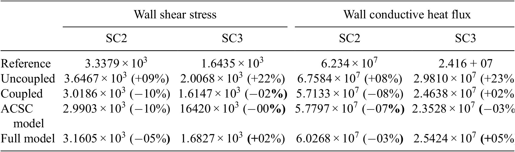
Overall, these results demonstrate that the Full model is able to reproduce a level of accuracy that is similar to that of the coupled algebraic model for the simulation of a cooled channel with large temperature variations. This confirms the ability of the graph neural network wall modeling approach to generalize from a priori training to an a posteriori testing configuration for this particular flow. In the next section, we will assess to which extent the graph neural network wall modeling approach can provide an improvement for a more complex simulation that is known to be difficult to simulate using an algebraic model devised for anisothermal fully developed turbulent boundary layers.
6.3. High-pressure turbine blade
This section addresses the wall-modeled LES of the high-pressure turbine blade L89, not included in the training dataset. The L89 blade configuration is an experimental configuration instrumented for boundary-layer measurements with realistic operating conditions in terms of Reynolds and Mach numbers. It is thus in many ways representative of real turbomachinery flow, for which similar measurements are typically not available. The simulation reproduces the test case MUR235 of Arts et al. (Reference Arts, Rouvroit and Rutherford1990). This test case features a complex physics compared to the symmetrically cooled channel flow, that involves transitional and fully turbulent boundary layers with large temperature variations. In the literature, the LES of the test case MUR235, characterized by a large inlet turbulence intensity of 6%, has been found to be particularly challenging compared to other test cases of the VKI LS1989-MUR series (Arts et al., Reference Arts, Rouvroit and Rutherford1990). For instance, an accurate prediction is the wall heat flux on the suction side of the blade is more easily obtained for the MUR129 than the MUR235 test case (Collado Morata et al., Reference Collado Morata, Gourdain, Duchaine and Gicquel2012; Gourdain et al., Reference Gourdain, Gicquel and Collado Morata2012; Segui et al., Reference Segui, Gicquel, Duchaine and de Laborderie2017; Dupuy et al., Reference Dupuy, Gicquel, Odier, Duchaine and Arts2020. Accurate predictions have not been obtained with the resolution of a wall-modeled LES in the literature. This suggests the present MUR235 test case is relevant to assess the performance of wall models in a flow with complex boundary layer dynamics, and can be used as a benchmark for the development of wall models.
The operating conditions of the simulation are reported in Table 5. The flow is representative of a typical high-pressure turbine in terms of Mach and Reynolds numbers. Although the inlet temperature is low compared to the typical temperature downstream of a combustion chamber, the temperature ratio between the inlet flow and the blade is realistic. The blade profile is given by the reinterpolated manufacturing coordinates of Wheeler et al. (Reference Wheeler, Sandberg, Sandham, Pichler, Michelassi and Laskowski2016) to ensure a smooth surface curvature. The chord
 $ c $
is
$ c $
is
 $ 67.647 $
mm. The computational domain is periodic in the spanwise and pitchwise directions to model an infinite linear cascade of two-dimensional linearly extruded blade profiles. The origin of the Cartesian coordinate system (
$ 67.647 $
mm. The computational domain is periodic in the spanwise and pitchwise directions to model an infinite linear cascade of two-dimensional linearly extruded blade profiles. The origin of the Cartesian coordinate system (
 $ x $
,
$ x $
,
 $ y $
,
$ y $
,
 $ z $
) is placed at the leading edge of the blade, where
$ z $
) is placed at the leading edge of the blade, where
 $ x $
is the axial coordinate,
$ x $
is the axial coordinate,
 $ y $
the pitchwise coordinate, and
$ y $
the pitchwise coordinate, and
 $ z $
the spanwise coordinate. The curvilinear coordinate
$ z $
the spanwise coordinate. The curvilinear coordinate
 $ {s}_1 $
follows the blade profile and is zero at the leading edge, positive on the suction side of the blade, and negative on the pressure side of the blade (Figure 12). The inlet is located at
$ {s}_1 $
follows the blade profile and is zero at the leading edge, positive on the suction side of the blade, and negative on the pressure side of the blade (Figure 12). The inlet is located at
 $ {x}_{\mathrm{inlet}}=-0.81c $
and the outlet at
$ {x}_{\mathrm{inlet}}=-0.81c $
and the outlet at
 $ {x}_{\mathrm{outlet}}=1.48c $
. The spanwise length of the domain is set
$ {x}_{\mathrm{outlet}}=1.48c $
. The spanwise length of the domain is set
 $ 0.148c $
as this value is consistent with the literature (Bhaskaran and Lele, Reference Bhaskaran and Lele2010; Fransen et al., Reference Fransen, Collado Morata, Duchaine, Gourdain, Gicquel, Vial and Bonneau2011; Pichler et al., Reference Pichler, Kopriva, Laskowski, Michelassi and Sandberg2016) and the sensitivity analysis of Collado Morata et al. (Reference Collado Morata, Gourdain, Duchaine and Gicquel2012). A wall-resolved simulation of the case on a mesh containing 587 million cells, performed by Dupuy et al. (Reference Dupuy, Gicquel, Odier, Duchaine and Arts2020), is used as a reference. In addition, the experimental data of Arts et al. (Reference Arts, Rouvroit and Rutherford1990) is used when available. The WMLES mesh contains 47 million tetrahedral cells in total. The mesh is more refined close to the blade surface and near the trailing edge on the suction side (Figure 11, left). The distribution of the height of the first cell off the wall along the blade surface is given in Figure 11 (right). Convective and diffusion are both discretized using second-order accurate schemes (Lax and Wendroff, Reference Lax and Wendroff1960).
$ 0.148c $
as this value is consistent with the literature (Bhaskaran and Lele, Reference Bhaskaran and Lele2010; Fransen et al., Reference Fransen, Collado Morata, Duchaine, Gourdain, Gicquel, Vial and Bonneau2011; Pichler et al., Reference Pichler, Kopriva, Laskowski, Michelassi and Sandberg2016) and the sensitivity analysis of Collado Morata et al. (Reference Collado Morata, Gourdain, Duchaine and Gicquel2012). A wall-resolved simulation of the case on a mesh containing 587 million cells, performed by Dupuy et al. (Reference Dupuy, Gicquel, Odier, Duchaine and Arts2020), is used as a reference. In addition, the experimental data of Arts et al. (Reference Arts, Rouvroit and Rutherford1990) is used when available. The WMLES mesh contains 47 million tetrahedral cells in total. The mesh is more refined close to the blade surface and near the trailing edge on the suction side (Figure 11, left). The distribution of the height of the first cell off the wall along the blade surface is given in Figure 11 (right). Convective and diffusion are both discretized using second-order accurate schemes (Lax and Wendroff, Reference Lax and Wendroff1960).
Table 5. Operating point conditions of the MUR235 test cases (Arts et al., Reference Arts, Rouvroit and Rutherford1990)
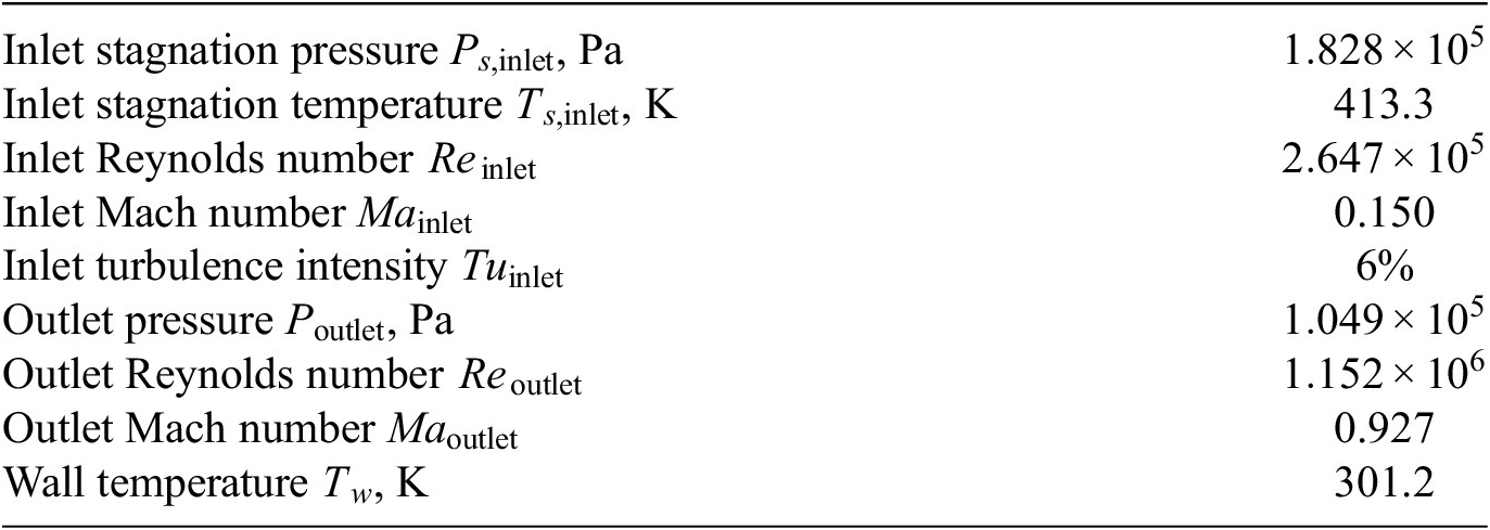
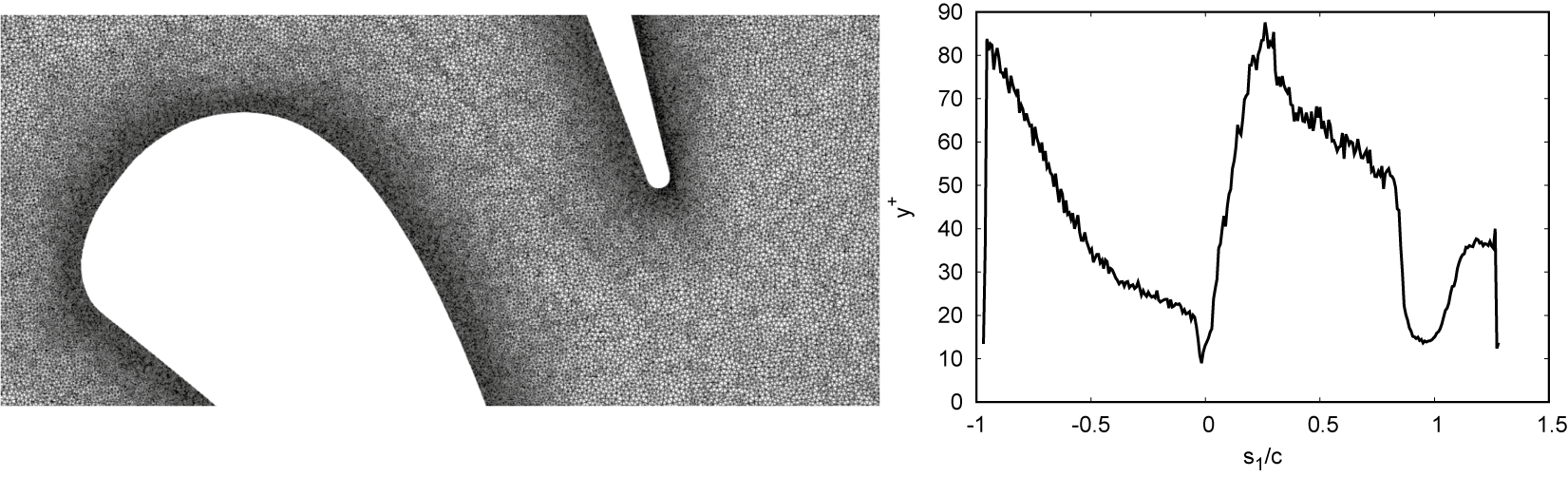
Figure 11. Left: Side view of the mesh, on the slice
 $ z/c=0.037 $
. Right: Height of the first cell off the wall along the blade surface, in wall units.
$ z/c=0.037 $
. Right: Height of the first cell off the wall along the blade surface, in wall units.
Wall-modeled LESs using the baseline uncoupled and coupled algebraic models, the ACSC and Full graph neural network wall models are performed using the Sigma (Nicoud et al., Reference Nicoud, Baya Toda, Cabrit, Bose and Lee2011) subgrid-scale viscosity model. The intensity of the incident turbulence in the wall-modeled LES is comparable to that of the reference high-fidelity simulation. Indeed, the turbulence intensity of the resolved scales,
 $ Tu $
, defined as
$ Tu $
, defined as
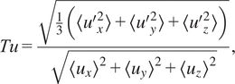 $$ Tu=\frac{\sqrt{\frac{1}{3}\left(\left\langle {u^{\prime}}_x^2\right\rangle +\left\langle {u^{\prime}}_y^2\right\rangle +\left\langle {u^{\prime}}_z^2\right\rangle \right)}}{\sqrt{{\left\langle {u}_x\right\rangle}^2+{\left\langle {u}_y\right\rangle}^2+{\left\langle {u}_z\right\rangle}^2}}, $$
is 5% near the leading edge in the wall-modeled simulations, compared to 5.6% in the reference high-fidelity simulation. The instantaneous visualizations given in Figure 12 (center) show that the wall-modeled LES reproduces the main flow phenomena associated with the case. The trailing-edge flow is associated with both vortex shedding and the generation of a series of acoustic waves impinging on the suction side of the blade. Furthermore, there is a series of shocks quasi-normal to the blade on the suction side. The shocks induce a rapid transition of the suction-side boundary layer from a transitional state to a fully turbulent state (Dupuy et al., Reference Dupuy, Gicquel, Odier, Duchaine and Arts2020. This rapid turbulence transition is associated with a large increase of the wall shear stress in the region downstream of the shocks (
 $ {s}_1/c>0.96 $
). Figure 13a compares the distribution of the wall shear stress along the blade surface in the different simulations. The baseline uncoupled algebraic model, coupled algebraic model, and the ACSC graph neural network wall model lead to very similar wall shear stress profiles. In the three simulations, the wall shear stress is overestimated on the pressure side near the trailing edge and on the suction side until the shocks. In addition, the increase in wall shear stress associated with the shocks occurs further downstream in all wall-modeled LESs than in the reference high-fidelity simulation, even though the shocks location is accurately predicted. The simulation with the Full graph neural network wall model leads to a more accurate wall shear stress distribution. In particular, the wall shear stress is accurate throughout the pressure side of the blade and the peak wall shear stress after the strongly accelerating region near the leading edge of the blade (
$ {s}_1/c>0.96 $
). Figure 13a compares the distribution of the wall shear stress along the blade surface in the different simulations. The baseline uncoupled algebraic model, coupled algebraic model, and the ACSC graph neural network wall model lead to very similar wall shear stress profiles. In the three simulations, the wall shear stress is overestimated on the pressure side near the trailing edge and on the suction side until the shocks. In addition, the increase in wall shear stress associated with the shocks occurs further downstream in all wall-modeled LESs than in the reference high-fidelity simulation, even though the shocks location is accurately predicted. The simulation with the Full graph neural network wall model leads to a more accurate wall shear stress distribution. In particular, the wall shear stress is accurate throughout the pressure side of the blade and the peak wall shear stress after the strongly accelerating region near the leading edge of the blade (
 $ {s}_1/c=0.3 $
) is not overestimated. These findings are affected by the selection of the subgrid-scale model. Indeed, the quasi-normal shocks on suction side of the blade do not provoke the expected turbulent transition of the boundary layer using the Smagorinsky model. This halts the generation of acoustic waves at the trailing edge of the blade (Figure 12, bottom). Accordingly, the rapid increase in wall shear stress near the trailing edge of the blade (
$ {s}_1/c=0.3 $
) is not overestimated. These findings are affected by the selection of the subgrid-scale model. Indeed, the quasi-normal shocks on suction side of the blade do not provoke the expected turbulent transition of the boundary layer using the Smagorinsky model. This halts the generation of acoustic waves at the trailing edge of the blade (Figure 12, bottom). Accordingly, the rapid increase in wall shear stress near the trailing edge of the blade (
 $ {s}_1/c>0.96 $
) is not reproduced with either the baseline algebraic model or the graph neural network wall model with the Smagorinsky model (Figure 14a). On the rest of the blade, the predictions are relatively similar to those obtained using the Sigma model. Namely, the Full graph neural network wall model predicts more accurately the wall shear stress on the pressure side compared to the coupled algebraic model, and the peak wall shear stress after the strongly accelerating region near
$ {s}_1/c>0.96 $
) is not reproduced with either the baseline algebraic model or the graph neural network wall model with the Smagorinsky model (Figure 14a). On the rest of the blade, the predictions are relatively similar to those obtained using the Sigma model. Namely, the Full graph neural network wall model predicts more accurately the wall shear stress on the pressure side compared to the coupled algebraic model, and the peak wall shear stress after the strongly accelerating region near
 $ {s}_1/c=0.3 $
on the suction side. Thus, the Full model is able to leverage the non-equilibrium configurations of the training database to improve the wall shear stress prediction in these regions, which are not fully turbulent.
$ {s}_1/c=0.3 $
on the suction side. Thus, the Full model is able to leverage the non-equilibrium configurations of the training database to improve the wall shear stress prediction in these regions, which are not fully turbulent.
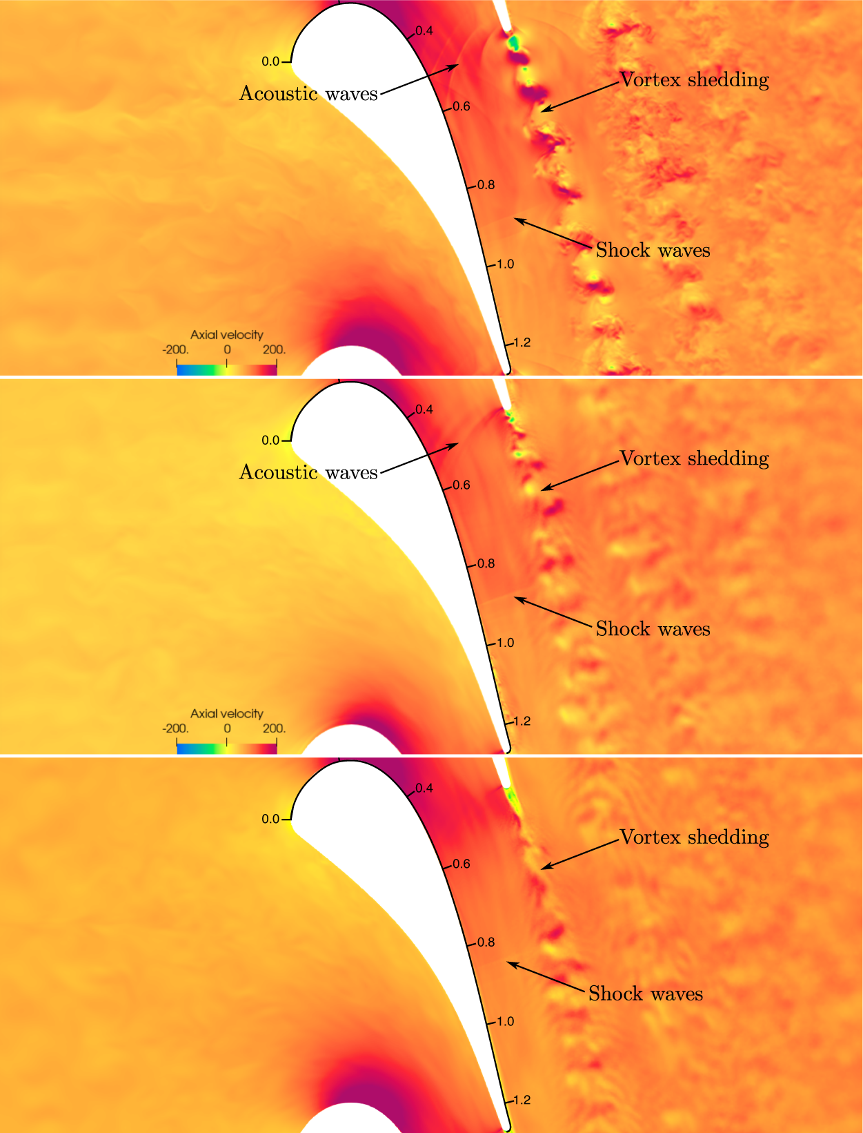
Figure 12.
Instantaneous field of axial velocity in the reference high-fidelity simulation of Dupuy et al. (Reference Dupuy, Gicquel, Odier, Duchaine and Arts2020) (top), the wall-modeled large-eddy simulation using the Sigma model (center), and the wall-modeled large-eddy simulation using the Smagorinsky model (bottom) on the plane
 $ z/c=0.037 $
. The curvilinear abscissa
$ z/c=0.037 $
. The curvilinear abscissa
 $ {s}_1/c $
along the blade is given in the figures for reference.
$ {s}_1/c $
along the blade is given in the figures for reference.
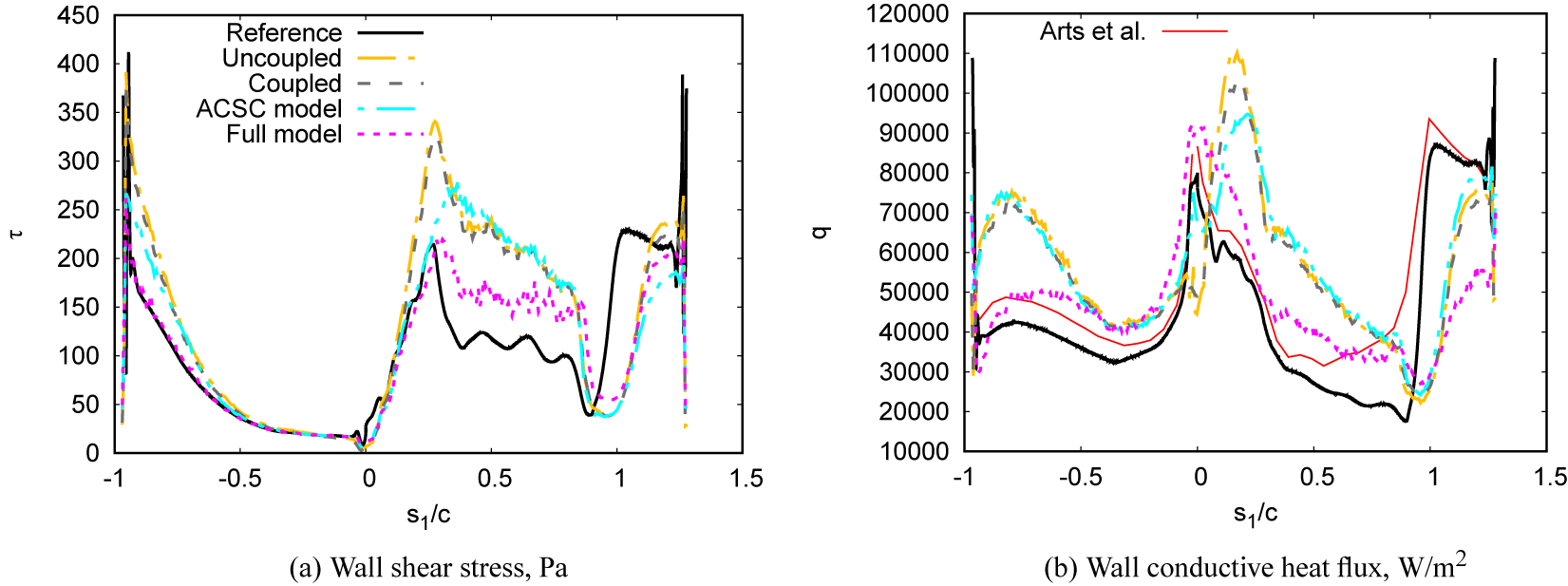
Figure 13. Wall shear stress and conductive heat flux along the blade surface using the Sigma model.
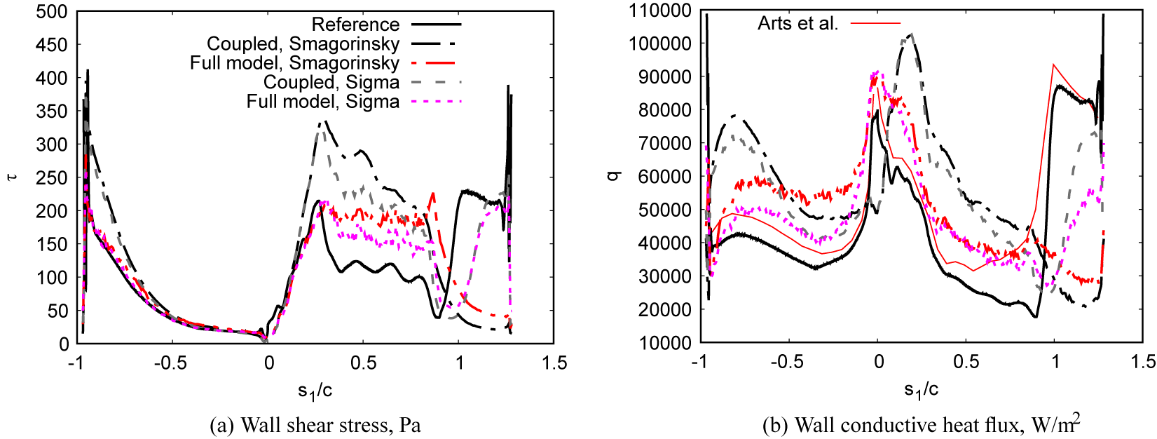
Figure 14. Wall shear stress and conductive heat flux along the blade surface, using the Smagorinsky and Sigma subgrid-scale models.
With regard to the wall heat flux prediction, Figures 13b and 14b, the Full model also improves the prediction compared to the baseline uncoupled algebraic model, coupled algebraic model, and the ACSC graph neural network wall model. With both the Sigma and Smagorinsky models, the peak wall heat flux location correctly occurs at the leading edge with the Full model, whereas it occurs further downstream, below
 $ {s}_1/c=0.2 $
, in the other wall-modeled LESs. In addition, the wall heat flux is significantly less overestimated on the suction side of the blade, in the transitional region before the shocks
$ {s}_1/c=0.2 $
, in the other wall-modeled LESs. In addition, the wall heat flux is significantly less overestimated on the suction side of the blade, in the transitional region before the shocks
 $ {s}_1/c<0.9 $
. The wall heat flux prediction is also improved on the pressure side of the blade, below
$ {s}_1/c<0.9 $
. The wall heat flux prediction is also improved on the pressure side of the blade, below
 $ {s}_1/c<-0.5 $
, especially using the Sigma subgrid-scale model. However, the simulation with the Full model leads to a large underestimation of the wall heat flux downstream of the shocks on the suction side, using the Sigma model, whereas the other wall-modeled LESs provide a more accurate prediction in that region. The deficiency is related to the incompressible isothermal simulation included in the training dataset for the Full model, since the ACSC model lead to a more accurate prediction in that region (Figure 13b). Overall, the results are nevertheless promising for the prospect of graph neural network wall modeling, since outside of this region the wall heat flux distribution on the blade surface is fairly well predicted compared to the reference simulation, providing a level of accuracy that is not trivial to reproduce even in a wall-resolved simulation (Collado Morata et al., Reference Collado Morata, Gourdain, Duchaine and Gicquel2012; Gourdain et al., Reference Gourdain, Gicquel and Collado Morata2012; Segui et al., Reference Segui, Gicquel, Duchaine and de Laborderie2017; Dupuy et al., Reference Dupuy, Gicquel, Odier, Duchaine and Arts2020). Machine-learning wall modeling provides a framework that has the potential to take into account both non-equilibrium effects and variable-density effects in complex geometries, and this ability could be progessively refined and improved over time following the developments of larger numerical training databases.
$ {s}_1/c<-0.5 $
, especially using the Sigma subgrid-scale model. However, the simulation with the Full model leads to a large underestimation of the wall heat flux downstream of the shocks on the suction side, using the Sigma model, whereas the other wall-modeled LESs provide a more accurate prediction in that region. The deficiency is related to the incompressible isothermal simulation included in the training dataset for the Full model, since the ACSC model lead to a more accurate prediction in that region (Figure 13b). Overall, the results are nevertheless promising for the prospect of graph neural network wall modeling, since outside of this region the wall heat flux distribution on the blade surface is fairly well predicted compared to the reference simulation, providing a level of accuracy that is not trivial to reproduce even in a wall-resolved simulation (Collado Morata et al., Reference Collado Morata, Gourdain, Duchaine and Gicquel2012; Gourdain et al., Reference Gourdain, Gicquel and Collado Morata2012; Segui et al., Reference Segui, Gicquel, Duchaine and de Laborderie2017; Dupuy et al., Reference Dupuy, Gicquel, Odier, Duchaine and Arts2020). Machine-learning wall modeling provides a framework that has the potential to take into account both non-equilibrium effects and variable-density effects in complex geometries, and this ability could be progessively refined and improved over time following the developments of larger numerical training databases.
For completeness, it is useful to discuss the computational cost associated with such machine-learning wall models. The present model has not been developed with computational cost as a primary concern. For instance, the wall shear stress and the wall conductive heat flux are presently predicted by sequentially applying two independent neural networks, although they certainly share common features or representations in the hidden layers. Moreover, the hyperparameters of each network have been selected without considering computational cost and, as a result, we did not attempt to prune the networks to reduce computational overhead. The present graph neural network wall model has been benchmarked, for the wall-modeled simulation of the LS89 blade. The tests are performed on the Jean–Zay super-computing cluster, which as many other recent super-computing clusters has a hybrid architecture. The hybrid nodes contain 40 CPU cores (Intel Cascade Lake 6248 2.5 GHz) and 4 GPUs (Nvidia Tesla V100 SXM2 32GB). The wall-modeled simulations exploit these hybrid resources by executing the graph neural network prediction exclusively on the GPUS, concurrently to parts of the LES schemes, as discussed in Serhani et al. (Reference Serhani, Xing, Dupuy, Lapeyre and Staffelbach2022). In that context, we may defined the deep-learning overhead as the additional cost induced by the use of the graph neural network wall model on a given hybrid node, which may be calculated by considering the cost of the graph neural network prediction and related to communications, from which is subtracted the cost of overlapped LES computations. Figure 15 gives the overhead of the model for 2–16 hybrid nodes. The deep learning overhead ranges from 25 to 30% of the total iteration cost. Moving forward, further developments should consider computational cost in the model development.
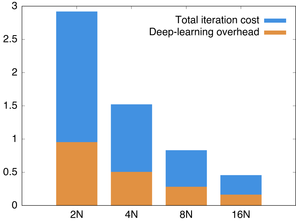
Figure 15. Overhead of the graph neural network wall model per iteration for 2, 4, 6, and 16 hybrid nodes.
7. Conclusion
Using a graph neural network to model the wall behavior of fluids requires an effort to encode some of the flow dependencies in the model architecture or the training process as it would require a considerable effort to build a dataset sufficiently diverse to comprehensively specify the wall behavior of fluids. The present graph neural network architecture implicitly makes an assumption of spatial locality and encodes the invariance of the model under a translation of the mesh. Furthermore, the selection, scaling, and augmentation of the input features forces the model to be equivariant under Galilean transformations, orthogonal transformations, and Mach number transformations. While a large amount of training data is still required, these assumptions allow the model to operate for a large range of scales of density, viscosity, length, velocity, temperature, or pressure. The procedure has been assessed by training the model on both incompressible isothermal and compressible anisothermal flows, for the modeling of the wall shear stress and the wall conductive heat flux. The a priori results demonstrated the capability of the model to generalize to both incompressible isothermal and compressible anisothermal simulations not seen during training. The a posteriori results confirmed the ability of the graph neural network wall model to generalize from a priori training to an a posteriori test for a fully developed channel flow with large temperature variations, as the model was able to reach a level of accuracy comparable to a state-of-the-art algebraic model. Finally, The wall-modeled LES of the high-pressure turbine blade VKI LS1989, for the test case MUR235 of the VKI LS1989-MUR series, showed that the model could leverage the non-equilibrium configurations of the training database to provide a more accurate prediction than the baseline algebraic wall models devised for equilibrium turbulent flow configurations in a complex flow with large temperature variations and compressibility effects. In particular, the model is able to predict fairly well the wall heat flux distribution on the surface of the blade, which is a challenging quantity to predict even in a wall-resolved simulation. The further development of graph neural networks for wall modeling is thus promising for the LES, and has the potential to improve the accuracy and efficiency of simulations of complex industrial flows.
Acknowledgments
This work was granted access to the computer resources of IDRIS under the allocation A0122A06074 made by GENCI. We are indebted to the European Union’s Horizon 2020 research and innovation programme (grant agreement n° 814837) for producing and making openly available some of the data used in this work. We are grateful to L. Agostini and P. Vincent for providing us the data for the channel-flow simulation at
 $ {\mathit{\operatorname{Re}}}_{\tau }=180 $
, to O. Lehmkuhl and A. Miró for providing us the data for the three-dimensional diffuser simulation, to F. C. Massa and A. Colombo for providing us the data for the adverse-pressure-gradient simulation, to F. Bataille and A. Toutant for providing us the data for the asymmetrically cooled/heated channel flow simulations, to L. Potier and R. Costes for providing us the data for the symmetrically cooled channel flow simulations, and to D. Papadogiannis for providing us the data for the NACA 65-009 blade cascade simulation which has been performed under the PRACE project CornerLES.
$ {\mathit{\operatorname{Re}}}_{\tau }=180 $
, to O. Lehmkuhl and A. Miró for providing us the data for the three-dimensional diffuser simulation, to F. C. Massa and A. Colombo for providing us the data for the adverse-pressure-gradient simulation, to F. Bataille and A. Toutant for providing us the data for the asymmetrically cooled/heated channel flow simulations, to L. Potier and R. Costes for providing us the data for the symmetrically cooled channel flow simulations, and to D. Papadogiannis for providing us the data for the NACA 65-009 blade cascade simulation which has been performed under the PRACE project CornerLES.
Author contribution
Conceptualization: D.D., N.O., C.L.; Data curation: D.D.; Data visualization: D.D.; Investigation: D.D.; Methodology: D.D., N.O., C.L.; Supervision: N.O., C.L.; Writing—original draft: D.D.; Writing—review and editing: D.D., N.O., C.L. All authors approved the final submitted draft.
Competing interest
The authors declare that they have no conflict of interest.
Data availability statement
The data that support the findings of this study are available from the corresponding author upon reasonable request.
Funding statement
This project has not received any external funding.
Ethical standard
The research meets all ethical guidelines, including adherence to the legal requirements of the study country.
A. Wall-resolved simulation of the SC1, SC2, and SC3 cases
This section presents the wall-resolved simulations of the symmetrically cooled channel flows (SC1, SC2, SC3). These simulations are used to train the graph neural network wall model (Section 4.2) and for a priori and a posteriori tests (Sections 5 and 6). In the three simulations, the fluid is a mixture, hereafter referred to as H2-O2-12S, composed of 8 species (H2, H, O2, OH, O, H2O, HO2, and H2O2) which are products of H2/O2 combustion. Since no chemical reactions are taken into account, the mixture behaves as a single-component fluid. The ideal gas-specific constant of the mixture is
 $ r=480.949 $
J kg−1 K−1. The dynamic viscosity of the mixture follows a power law
$ r=480.949 $
J kg−1 K−1. The dynamic viscosity of the mixture follows a power law
 $ \mu (T)=1.82\times {10}^{-5}{\left(T/300\right)}^{0.715} $
Pas. Heat conductivity is computed as
$ \mu (T)=1.82\times {10}^{-5}{\left(T/300\right)}^{0.715} $
Pas. Heat conductivity is computed as
 $ \lambda =\mu {C}_p/\mathit{\Pr} $
, with
$ \lambda =\mu {C}_p/\mathit{\Pr} $
, with
 $ \mathit{\Pr}=0.706 $
the Prandtl number of the mixture, assumed constant, and where the isobaric heat capacity
$ \mathit{\Pr}=0.706 $
the Prandtl number of the mixture, assumed constant, and where the isobaric heat capacity
 $ {C}_p $
is computed from tabulated data (Stull and Prophet, Reference Stull and Prophet1971). The cases SC2 and SC3 both involve a large temperature ratio of 3 between the bulk flow and the channel walls. Since the thermophysical properties of the fluid are thermo-dependent, the temperature variations generate a strong coupling between the fields of temperature and velocity. To validate the numerical method, a channel with less temperature variations (SC1) is simulated. Indeed, given the low-temperature ratio of 1.1 between the bulk flow and the channel walls in the SC1 simulation, the mean profiles of velocity and temperature are close to those of an incompressible channel with a passive scalar.
$ {C}_p $
is computed from tabulated data (Stull and Prophet, Reference Stull and Prophet1971). The cases SC2 and SC3 both involve a large temperature ratio of 3 between the bulk flow and the channel walls. Since the thermophysical properties of the fluid are thermo-dependent, the temperature variations generate a strong coupling between the fields of temperature and velocity. To validate the numerical method, a channel with less temperature variations (SC1) is simulated. Indeed, given the low-temperature ratio of 1.1 between the bulk flow and the channel walls in the SC1 simulation, the mean profiles of velocity and temperature are close to those of an incompressible channel with a passive scalar.
The geometry of the SC1 and SC2 simulations is a rectangular parallelepiped of size
 $ 3.5h\times 2h\times 1.3h $
, where
$ 3.5h\times 2h\times 1.3h $
, where
 $ h=2\times {10}^{-4} $
m is the half-height of the channel (Figure A1). The bottom (
$ h=2\times {10}^{-4} $
m is the half-height of the channel (Figure A1). The bottom (
 $ y=-h $
) and top (
$ y=-h $
) and top (
 $ y=h $
) boundaries are walls with a constant and uniform imposed temperature of
$ y=h $
) boundaries are walls with a constant and uniform imposed temperature of
 $ {T}_1=2863 $
K in the case SC1 and
$ {T}_1=2863 $
K in the case SC1 and
 $ {T}_2=1050 $
K in the case SC2. The flow between the two walls is periodic in the streamwise (
$ {T}_2=1050 $
K in the case SC2. The flow between the two walls is periodic in the streamwise (
 $ x $
) and spanwise (
$ x $
) and spanwise (
 $ z $
) directions. The small dimensions of the computational domain were selected in order to reduce the computational cost of the wall-resolved simulations and are probably sufficient to obtain accurate first- and second-order turbulence statistics (Lozano-Durán and Jiménez, Reference Lozano-Durán and Jiménez2014. Source terms are added in the momentum conservation equation and energy conservation equation in order to counteract the wall friction/conduction and prevent the flow from vanishing. The source term in the momentum conservation equation, constant and uniform, leads to a friction Reynolds number
$ z $
) directions. The small dimensions of the computational domain were selected in order to reduce the computational cost of the wall-resolved simulations and are probably sufficient to obtain accurate first- and second-order turbulence statistics (Lozano-Durán and Jiménez, Reference Lozano-Durán and Jiménez2014. Source terms are added in the momentum conservation equation and energy conservation equation in order to counteract the wall friction/conduction and prevent the flow from vanishing. The source term in the momentum conservation equation, constant and uniform, leads to a friction Reynolds number
 $ {\mathit{\operatorname{Re}}}_{\tau, 1}=320 $
in the case SC1 and
$ {\mathit{\operatorname{Re}}}_{\tau, 1}=320 $
in the case SC1 and
 $ {\mathit{\operatorname{Re}}}_{\tau, 2}=1150 $
in the case SC2. In the energy conservation equation, the source term targets a bulk temperature
$ {\mathit{\operatorname{Re}}}_{\tau, 2}=1150 $
in the case SC2. In the energy conservation equation, the source term targets a bulk temperature
 $ {T}_b=3150 $
K in both cases, where
$ {T}_b=3150 $
K in both cases, where
 $ {T}_b $
is defined as
$ {T}_b $
is defined as
 $ {T}_b={\int}_{-h}^h\left\langle \rho {u}_xT\right\rangle dy/{\int}_{-h}^h\left\langle \rho {u}_x\right\rangle dy $
. The Mach number of the simulations is low (below 0.3). The Cartesian orthogonal mesh is uniform in the streamwise and spanwise direction and follows a hyperbolic tangent law in the wall-normal direction. The same mesh resolution is used in the simulations SC1 and SC2. Namely, the cell size in wall units is
$ {T}_b={\int}_{-h}^h\left\langle \rho {u}_xT\right\rangle dy/{\int}_{-h}^h\left\langle \rho {u}_x\right\rangle dy $
. The Mach number of the simulations is low (below 0.3). The Cartesian orthogonal mesh is uniform in the streamwise and spanwise direction and follows a hyperbolic tangent law in the wall-normal direction. The same mesh resolution is used in the simulations SC1 and SC2. Namely, the cell size in wall units is
 $ \Delta {x}^{+}=8 $
in the streamwise direction,
$ \Delta {x}^{+}=8 $
in the streamwise direction,
 $ \Delta {z}^{+}=4 $
in the spanwise direction and ranges from
$ \Delta {z}^{+}=4 $
in the spanwise direction and ranges from
 $ \Delta {y}^{+}=0.9 $
at the wall to
$ \Delta {y}^{+}=0.9 $
at the wall to
 $ \Delta {y}^{+}=11 $
at the center of the domain in the wall-normal direction. This results in a total number of cells of
$ \Delta {y}^{+}=11 $
at the center of the domain in the wall-normal direction. This results in a total number of cells of
 $ 150\times 119\times 100 $
in the case SC1 and
$ 150\times 119\times 100 $
in the case SC1 and
 $ 500\times 389\times 400 $
in the case SC2. The simulations are performed using a two-step Taylor–Galerkin convective scheme with third-order spatiotemporal accuracy and centered second-order diffusive scheme. The subgrid-scale viscosity is computed using the WALE model (Nicoud and Ducros, Reference Nicoud and Ducros1999), with a model constant
$ 500\times 389\times 400 $
in the case SC2. The simulations are performed using a two-step Taylor–Galerkin convective scheme with third-order spatiotemporal accuracy and centered second-order diffusive scheme. The subgrid-scale viscosity is computed using the WALE model (Nicoud and Ducros, Reference Nicoud and Ducros1999), with a model constant
 $ {C}_w=0.57 $
. The subgrid-scale thermal conductivity is computed assuming a constant subgrid-scale Prandtl number
$ {C}_w=0.57 $
. The subgrid-scale thermal conductivity is computed assuming a constant subgrid-scale Prandtl number
 $ {\mathit{\Pr}}_{\mathrm{sgs}}=0.6 $
, that is
$ {\mathit{\Pr}}_{\mathrm{sgs}}=0.6 $
, that is
 $ {\lambda}_{\mathrm{sgs}}={C}_p{\mu}_{\mathrm{sgs}}/{\mathit{\Pr}}_{\mathrm{sgs}} $
. The subgrid-scale viscosity is 40 times smaller than the molecular viscosity on average and at least five times smaller than the molecular viscosity at each grid point.
$ {\lambda}_{\mathrm{sgs}}={C}_p{\mu}_{\mathrm{sgs}}/{\mathit{\Pr}}_{\mathrm{sgs}} $
. The subgrid-scale viscosity is 40 times smaller than the molecular viscosity on average and at least five times smaller than the molecular viscosity at each grid point.
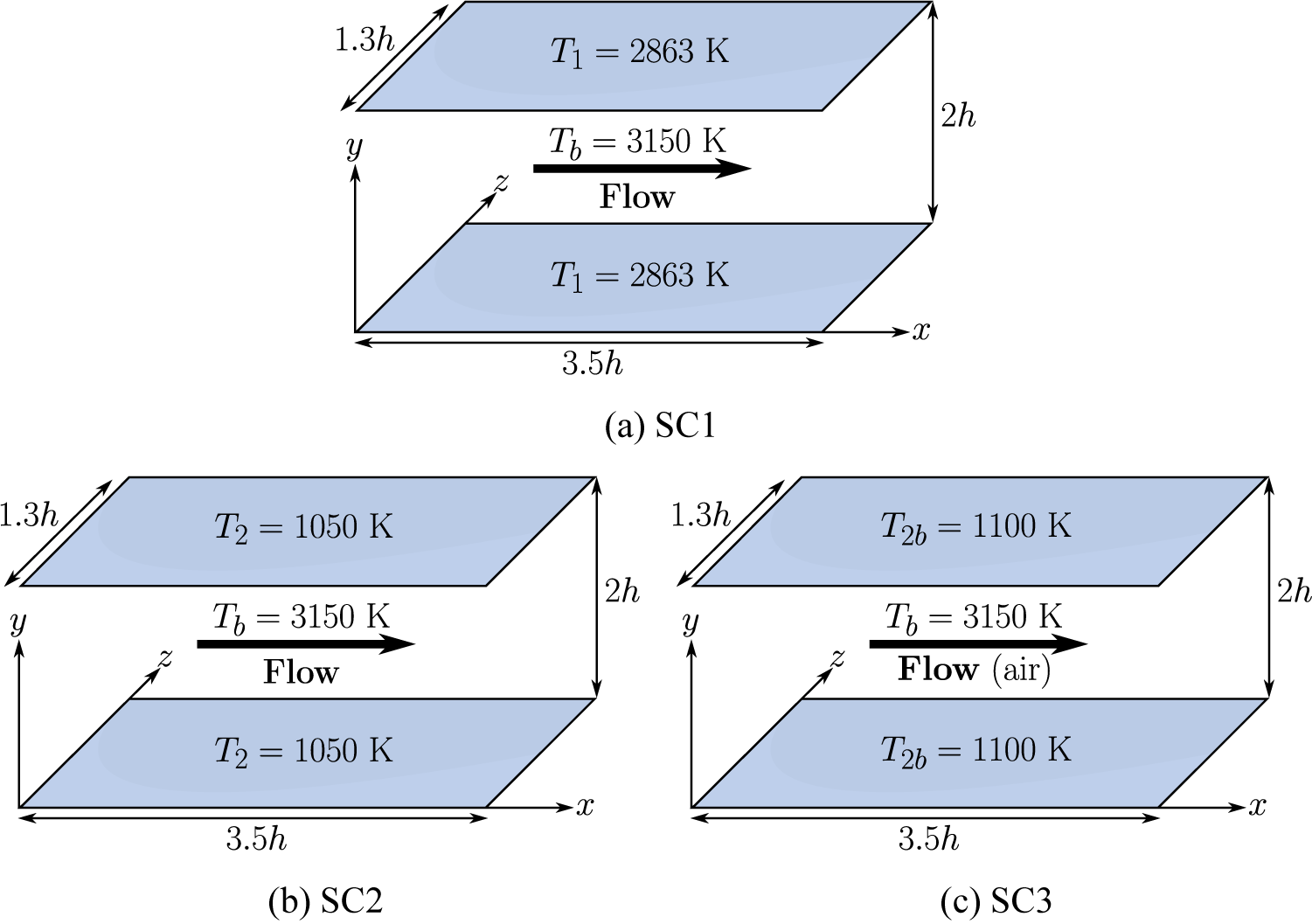
Figure A1. Geometry of the symmetrically cooled channel flows SC1, SC2, and SC3.
In addition to the channels SC1 and SC2, we performed a wall-resolved LES that is similar to the SC2 simulation in terms of friction Reynolds number and temperature ratio but with a different working fluid. This simulation is used in Section 6.2 to validate the graph neural network wall model and is hereafter referred to as the simulation SC3. In that simulation, the fluid (air) is characterized by an ideal gas-specific constant
 $ r=288.184 $
Jkg−1 K−1, a constant Prandtl number
$ r=288.184 $
Jkg−1 K−1, a constant Prandtl number
 $ \mathit{\Pr}=0.71 $
, and a Sutherland dynamic-viscosity law
$ \mathit{\Pr}=0.71 $
, and a Sutherland dynamic-viscosity law
 $ \mu (T)=1.716\times {10}^{-5}{\left(T/273.15\right)}^{3/2}\left(273.15+110.6\right)/\left(T+110.6\right) $
Pas (Sutherland, Reference Sutherland1893). Source terms are added in the momentum conservation equation and energy conservation equation to target a friction Reynolds number
$ \mu (T)=1.716\times {10}^{-5}{\left(T/273.15\right)}^{3/2}\left(273.15+110.6\right)/\left(T+110.6\right) $
Pas (Sutherland, Reference Sutherland1893). Source terms are added in the momentum conservation equation and energy conservation equation to target a friction Reynolds number
 $ {\mathit{\operatorname{Re}}}_{\tau, 2}=1150 $
and a bulk temperature
$ {\mathit{\operatorname{Re}}}_{\tau, 2}=1150 $
and a bulk temperature
 $ {T}_b=3150 $
K. The temperature of the channel walls is constant and equal to 1100 K. The computation domain, mesh, and numerical method are identical to those of the simulation SC2.
$ {T}_b=3150 $
K. The temperature of the channel walls is constant and equal to 1100 K. The computation domain, mesh, and numerical method are identical to those of the simulation SC2.
The profiles of mean streamwise velocity, mean temperature, standard deviation of streamwise velocity, and standard deviation of temperature in the simulations SC1, SC2, and SC3 are provided in Figure A2. To validate the numerical method, we compare the results of the simulation SC1, in which the coupling between the velocity and temperature is low, to the uncoupled direct numerical simulation of Kawamura et al. (Reference Kawamura, Ohsaka, Abe and Yamamoto1998) at
 $ {\mathit{\operatorname{Re}}}_{\tau }=395 $
and
$ {\mathit{\operatorname{Re}}}_{\tau }=395 $
and
 $ \mathit{\Pr}=0.71 $
. The profiles of the SC1 simulations are close to the reference profiles of Kawamura et al. (Reference Kawamura, Ohsaka, Abe and Yamamoto1998), which is expected given the low-temperature ratio of 1.1. The profiles of the simulations SC2 and SC3, however, deviate strongly from these reference profiles due to the effect of the large variations of temperature in the channel (temperature ratio of 3). The mean streamwise velocity does not follow Reichardt’s law (31), nor does the mean temperature profile follows Kader’s law (32), since these analytical profiles do not accurately take into account the effect of the coupling between velocity and temperature. In addition, the peak standard deviation of streamwise velocity or of temperature has a larger amplitude and is farther from the wall than in no-coupling case of Kawamura et al. (Reference Kawamura, Ohsaka, Abe and Yamamoto1998). Part of the effect of the large temperature variations can be characterized by using the semi-local scaling, based on the wall friction velocity and the mean local fluid properties (Rotta, Reference Rotta1959; Huang et al., Reference Huang, Coleman and Bradshaw1995; Patel et al., Reference Patel, Boersma and Pecnik2017; Dupuy et al., Reference Dupuy, Toutant and Bataille2018, Reference Dupuy, Toutant and Bataille2019). The semi-local friction velocity is defined as
$ \mathit{\Pr}=0.71 $
. The profiles of the SC1 simulations are close to the reference profiles of Kawamura et al. (Reference Kawamura, Ohsaka, Abe and Yamamoto1998), which is expected given the low-temperature ratio of 1.1. The profiles of the simulations SC2 and SC3, however, deviate strongly from these reference profiles due to the effect of the large variations of temperature in the channel (temperature ratio of 3). The mean streamwise velocity does not follow Reichardt’s law (31), nor does the mean temperature profile follows Kader’s law (32), since these analytical profiles do not accurately take into account the effect of the coupling between velocity and temperature. In addition, the peak standard deviation of streamwise velocity or of temperature has a larger amplitude and is farther from the wall than in no-coupling case of Kawamura et al. (Reference Kawamura, Ohsaka, Abe and Yamamoto1998). Part of the effect of the large temperature variations can be characterized by using the semi-local scaling, based on the wall friction velocity and the mean local fluid properties (Rotta, Reference Rotta1959; Huang et al., Reference Huang, Coleman and Bradshaw1995; Patel et al., Reference Patel, Boersma and Pecnik2017; Dupuy et al., Reference Dupuy, Toutant and Bataille2018, Reference Dupuy, Toutant and Bataille2019). The semi-local friction velocity is defined as
 $ {u}_{\tau}^{\ast }={\left(\tau /\left\langle \rho \right\rangle \right)}^0.5 $
and accordingly, the semi-local wall distance is
$ {u}_{\tau}^{\ast }={\left(\tau /\left\langle \rho \right\rangle \right)}^0.5 $
and accordingly, the semi-local wall distance is
 $ {y}^{\ast }={yu}_{\tau}^{\ast }/\left\langle \nu \right\rangle $
, the semi-local velocity is
$ {y}^{\ast }={yu}_{\tau}^{\ast }/\left\langle \nu \right\rangle $
, the semi-local velocity is
 $ {\boldsymbol{u}}^{\ast }=\boldsymbol{u}/{u}_{\tau}^{\ast } $
, and the semi-local temperature
$ {\boldsymbol{u}}^{\ast }=\boldsymbol{u}/{u}_{\tau}^{\ast } $
, and the semi-local temperature
 $ {T}^{\ast }=\left\langle \rho \right\rangle {C}_p{u}_{\tau}^{\ast}\left(T-{T}_{\mathrm{wall}}\right)/q $
. With the semi-local scaling (Figure A3), the mean velocity profiles of the simulation SC1, SC2, and SC3 are close to the uncoupled reference profile of Kawamura et al. (Reference Kawamura, Ohsaka, Abe and Yamamoto1998). The discrepancies in the amplitude and location of the peak standard deviation of streamwise velocity are also significantly reduced with the semi-local scaling. However, the semi-local scaling fails to collapse the profiles of mean tempeature of standard deviation of temperature, as large differences between coupled and uncoupled simulations remain in these cases. Overall, these results validate the numerical method in the uncoupled limit.
$ {T}^{\ast }=\left\langle \rho \right\rangle {C}_p{u}_{\tau}^{\ast}\left(T-{T}_{\mathrm{wall}}\right)/q $
. With the semi-local scaling (Figure A3), the mean velocity profiles of the simulation SC1, SC2, and SC3 are close to the uncoupled reference profile of Kawamura et al. (Reference Kawamura, Ohsaka, Abe and Yamamoto1998). The discrepancies in the amplitude and location of the peak standard deviation of streamwise velocity are also significantly reduced with the semi-local scaling. However, the semi-local scaling fails to collapse the profiles of mean tempeature of standard deviation of temperature, as large differences between coupled and uncoupled simulations remain in these cases. Overall, these results validate the numerical method in the uncoupled limit.
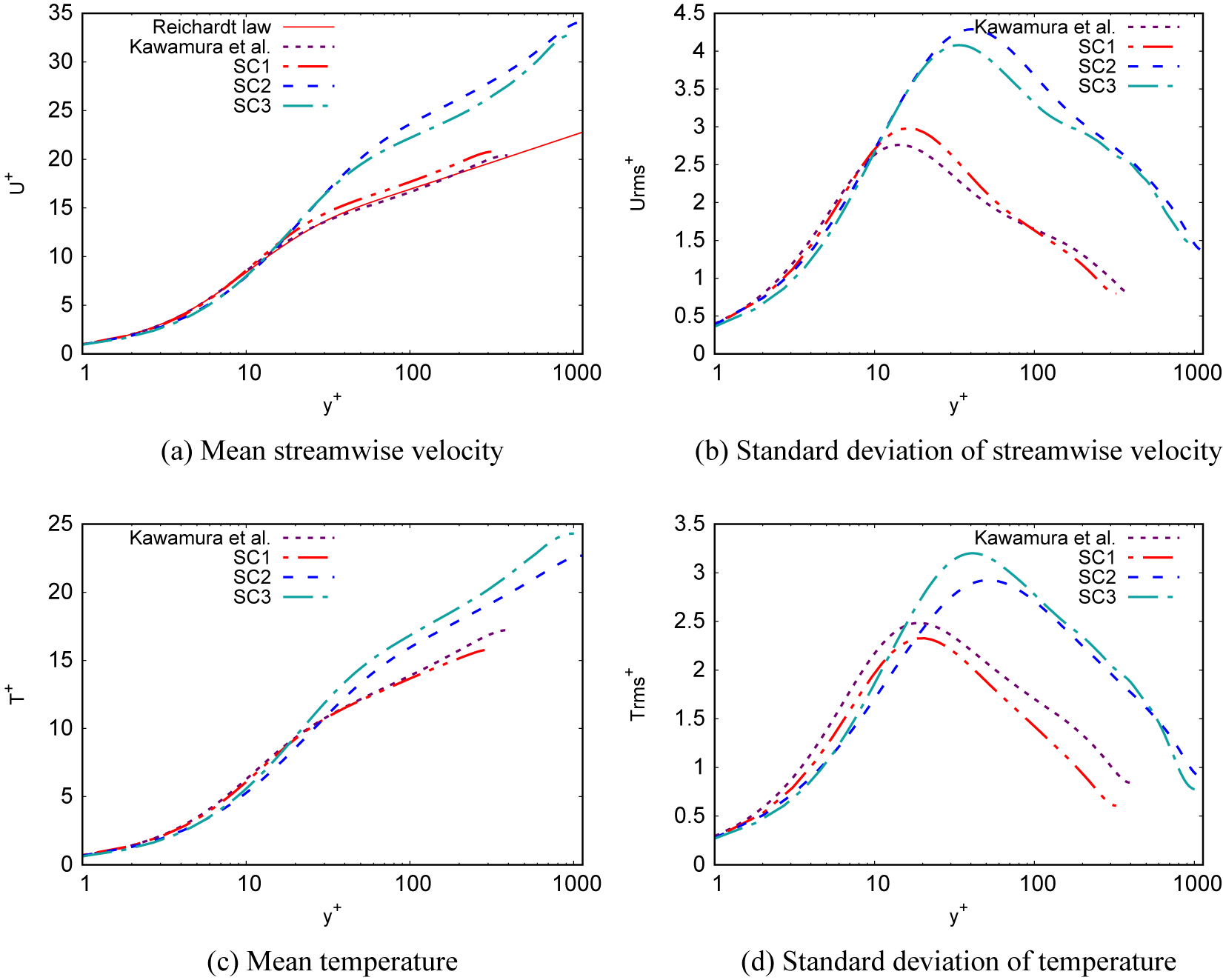
Figure A2. Profiles with classical wall scaling of mean streamwise velocity (a), mean temperature (c), standard deviation of streamwise velocity (b) and standard deviation of temperature in the simulations SC1, SC2, and SC3 (d). The direct numerical simulation profiles of Kawamura et al. (Reference Kawamura, Ohsaka, Abe and Yamamoto1998) at
 $ {\mathit{\operatorname{Re}}}_{\tau }=395 $
and
$ {\mathit{\operatorname{Re}}}_{\tau }=395 $
and
 $ \mathit{\Pr}=0.71 $
, in which temperature is a passive scalar, are given for comparison. The analytical profiles of Reichardt, given by equation ((31), and Kader, given by equation ((32), are also provided for reference.
$ \mathit{\Pr}=0.71 $
, in which temperature is a passive scalar, are given for comparison. The analytical profiles of Reichardt, given by equation ((31), and Kader, given by equation ((32), are also provided for reference.
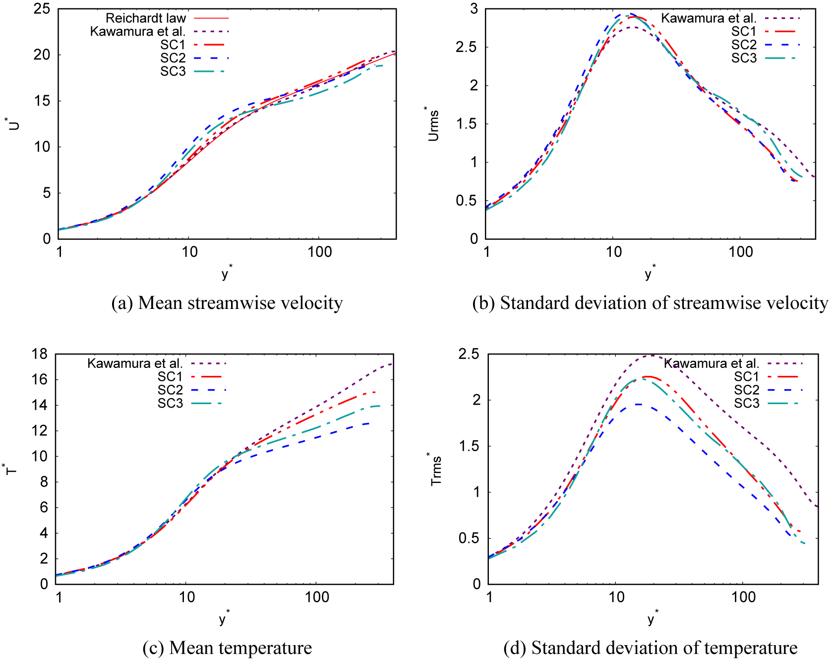
Figure A3. Profiles with semi-local scaling of mean streamwise velocity (a), mean temperature (c), standard deviation of streamwise velocity (b) and standard deviation of temperature in the simulations SC1, SC2, and SC3 (d). The direct numerical simulation profiles of Kawamura et al. (Reference Kawamura, Ohsaka, Abe and Yamamoto1998) at
 $ {\mathit{\operatorname{Re}}}_{\tau }=395 $
and
$ {\mathit{\operatorname{Re}}}_{\tau }=395 $
and
 $ \mathit{\Pr}=0.71 $
, in which temperature is a passive scalar, are given for comparison. The analytical profiles of Reichardt, given by equation ((31), and Kader, given by equation ((32), are also provided for reference.
$ \mathit{\Pr}=0.71 $
, in which temperature is a passive scalar, are given for comparison. The analytical profiles of Reichardt, given by equation ((31), and Kader, given by equation ((32), are also provided for reference.
B. Wall-modeled simulation of an incompressible isothermal channel flow
The simulation of an incompressible fully developed turbulent channel flow at friction Reynolds number
 $ {\mathit{\operatorname{Re}}}_{\tau }=950 $
is performed with the graph neural network wall models. The dimensions of the channel are
$ {\mathit{\operatorname{Re}}}_{\tau }=950 $
is performed with the graph neural network wall models. The dimensions of the channel are
 $ 12.6h\times 2h\times 6.3h $
, with
$ 12.6h\times 2h\times 6.3h $
, with
 $ h $
is the channel half-height. The mesh contains 12 million tetrahedral cells, and the average height of the first point off the wall, in wall units, is
$ h $
is the channel half-height. The mesh contains 12 million tetrahedral cells, and the average height of the first point off the wall, in wall units, is
 $ {y}^{+}=37 $
. The results of wall-modeled LESs using the ACSC and Full graph neural network wall models are compared to the reference profiles of Hoyas and Jiménez (Reference Hoyas and Jiménez2008) in Figure B1. In both cases, the profile of mean streamwise velocity exhibits a logarithmic-layer mismatch. The mismatch is almost identical to the mismatch obtained with an algebraic law-of-the-wall model based on the velocity within the first cell off the wall. Hence, the graph neural network wall models can operate in an incompressible isothermal channel flow, and provide a similar level of accuracy as an algebraic law-of-the-wall model.
$ {y}^{+}=37 $
. The results of wall-modeled LESs using the ACSC and Full graph neural network wall models are compared to the reference profiles of Hoyas and Jiménez (Reference Hoyas and Jiménez2008) in Figure B1. In both cases, the profile of mean streamwise velocity exhibits a logarithmic-layer mismatch. The mismatch is almost identical to the mismatch obtained with an algebraic law-of-the-wall model based on the velocity within the first cell off the wall. Hence, the graph neural network wall models can operate in an incompressible isothermal channel flow, and provide a similar level of accuracy as an algebraic law-of-the-wall model.
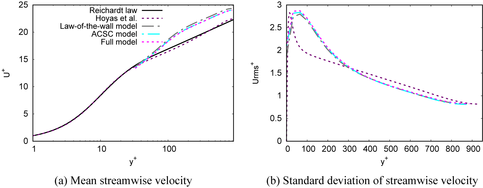
Figure B1. Mean streamwise velocity and standard deviation of streamwise velocity in large-eddy simulations of a channel flow at friction Reynolds number Reτ=950 with an algebraic wall stress model and a graph neural network wall model. The unfiltered direct numerical simulation profile of Hoyas and Jiménez (Reference Hoyas and Jiménez2008) is given for comparison.


 Open access
Comments
No Comments have been published for this article.