2.1 Introduction

Monopsony is a market structure in which there is a single buyer of a well-specified good or service.Footnote ¹ For decades, monopsony in the labor market was dismissed as a theoretical nicety without much – if any – empirical relevance. Recently, however, there has been a ground swell of concern due to wage stagnation, labor’s shrinking share of GDP, and reports of collusion among employers.Footnote ² Renewed interest in monopsony by academics, the antitrust agencies, and policy makers has been accompanied by legislative proposals to amend antitrust laws.Footnote ³ Complaints of monopsonistic abuse have been raised in the markets for hospital nurses, temporary duty nurses, physicians, hardware and software engineers, digital animators, and agricultural workers, among others.

To understand the source of the abuse and craft an economically sensible policy response, it is important to understand the economics of monopsony and monopsony power, that is, the power of the monopsonist to depress the wage it pays by curtailing employment. At first blush, one might suppose that lower labor costs enhance consumer welfare. But this is only true when lower labor costs flow from competition or productive efficiency – not when they result from monopsony. To avoid confused antitrust analysis, a clear understanding of monopsony is required. To this end, this chapter will focus on an economic analysis of monopsony.

We begin with a discussion of pure monopsony, that is, the case of a single employer. This analysis provides the economic foundation for analyzing other instances of disproportionate power in the labor market. In Section 2.3, we examine how monopsony in the input market influences marginal and average cost in the output market. Section 2.4 explains all-or-nothing offers in the labor market, and we then turn our attention to the dominant employer, which is a close cousin of pure monopsony in Section 2.5. Oligopsony, which is a labor market with a few large employers, is the focus of Section 2.6. In Section 2.7, we examine measures of monopsony power. As an economic matter, our concern is with the effects on the wages paid, the employment levels, the redistribution of wealth, and social welfare.

2.2 Basic Monopsony Model

If a firm is the only employer in a local labor market, it is a monopsonist by definition. For example, if a hospital or a hospital system in a city is the only employer of hospital nurses, it will be a monopsonist in that market. Similarly, a coal mine in a company town may be the only employer in the local labor market. To appreciate the economic consequences of monopsony, we begin with a competitive labor market and subsequently introduce monopsony.

2.2.1 Comparing Competition and Monopsony

All firms employ labor and other inputs to produce goods and services which they sell, and thereby earn profit. A manager has a fiduciary responsibility to maximize the value of their firm. Since the firm is worth more the higher its profit, a major responsibility of the manager is to make decisions intended to maximize the firm’s profits. These decisions include product design and quality, system of distribution, number and location of production facilities, and employment decisions. When it comes to employment decisions, the manager must do more than just arbitrarily pick the number of employees since this decision is directly influenced by costs and benefits.

The demand for labor is determined by the contribution of labor to the employer’s profit, which depends on the price of the employer’s output and the increment in output that is attributed to labor services. This demand is referred to as the value of the marginal product of labor, which is equal to the price of the firm’s output times the increase in the units of output made possible by the increased employment of labor. We denote this demand as VMP_L in Figure 2.1. The supply of labor is the positively sloped function labeled S_L in Figure 2.1. The supply of labor reveals the reservation wage that must be paid to employ any given quantity of labor services.

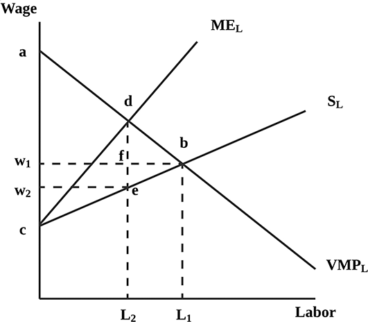
Figure 2.1 Profit maximization by a monopsonist

In a competitive labor market, the employer will expand its employment of labor until the VMP_L is equal to the wage that must be paid.Footnote ⁴ This occurs at the intersection of the VMP_L and S_L. At that point, employer surplus, area abw₁ and employee surplus, area w₁bc, are maximized.Footnote ⁵ The sum of employer surplus and employee surplus is a measure of social welfare. In this labor market, no other combination of wage rate and employment will yield more total surplus than the w₁ and L₁ combination yields.

Things change if the labor market is monopsonistic. To maximize its profit, the monopsonist will expand its employment of labor such that the marginal (or incremental) value of the increased output is just equal to the marginal cost of expanding employment. In other words, the employer wants to hire the quantity of labor services where the value of the marginal product is equal to the marginal expenditure on labor (ME_L).Footnote ⁶

The monopsonist will reduce employment to the point where the VMP_L is equal to the ME_L (which lies above S_L and is twice as steep).Footnote ⁷ The corresponding employment level is shown as L₂ in Figure 2.1 and the wage is w₂.

2.3 Monopsony, Marginal Cost, and Average Cost

In Figure 2.1, we see that the competitive wage of labor is equal to w₁. The exercise of monopsony power reduces the wage paid from w₁ to w₂. In ordinary circumstances, one would think that reduced wages would be a good thing for everyone except the employees. After all, lower wages result in higher profits for employers. It would seem that at least part of the cost savings will be passed on to consumers in the form of lower output prices. As a result, it appears that the monopsonist makes more profit and consumers are better off. So why is there an economic objection to monopsony?

The rosy scenario we just described is wrong. It is based on a fundamental misunderstanding of the relationship between the exercise of monopsony power and the resulting cost functions. The truth is that monopsony leads to lower average cost for some ranges of output, which provides the profit incentive for monopsonistic behavior, but monopsony causes marginal cost to shift upward, which leads to reduced output and a consequent decrease in consumer surplus.Footnote ⁸ We believe that it is important to understand these effects if antitrust policy is to be sound.

2.3.1 Impact on Average Cost and Marginal Cost

It can be shown that the presence of monopsony power causes the employer’s marginal cost curve to shift upward.Footnote ⁹ Whether the firm has market power in the output market or not, an upward shift in the firm’s marginal cost curve leads to a reduction in its profit maximizing output. Accordingly, there is no improvement in consumer welfare. In fact, the opposite will be the case regardless of whether the employer has market power in its output market. In either event, the effect of a reduction in the employer’s output is to increase price, reduce consumption, and thereby reduce social welfare.

In Figure 2.2, a firm that is a competitor in its output market and has no monopsony power in the labor market will be in equilibrium by producing Q₁ units of output. It sells its output for the market determined price P₁. In equilibrium, P₁ equals MC and AC. If this firm becomes a monopsonist in the local labor market, its marginal cost will shift upward from MC to MC'. To maximize its profit, the firm will hire less labor and produce less output. In Figure 2.2, output falls from Q₁ to Q₂. Despite the shift in marginal cost, the monopsonist enjoys higher profits as a result of curtailing its employment of labor.

Figure 2.2 Influence of monopsony on cost curves

The average cost of production also changes with the introduction of monopsony at all points except Q₁. At an output of Q₁, there will be no change in the employment of labor and, therefore, no change in the wage paid. As a result, the average cost with and without monopsony power is the same. If the employer increases the firm’s output beyond Q₁, it will have to hire more labor, which will cause the wage rate to rise. This, in turn, will cause the average cost (AC') to rise above the average cost (AC). In contrast, if the employer reduces the firm’s output below Q₁, it will reduce the amount of labor employed, which will cause the wage paid to fall. The result is that average cost falls and AC' will be below AC. This results in a general shift downward and to the left of the minimum point on the average cost curve, from AC to AC'. The employer’s average cost will be below the price of its output and the firm will earn economic profits equal to (P₁-AC')Q₂ > 0. The reduction in average cost resulting from a reduced employment of labor and the corresponding decrease in output provides the profit incentive for the monopsonist’s restricted employment of labor.

For antitrust policy purposes, it is important to understand that the reduced wages flowing from an exercise of monopsony power are not socially beneficial. While they result in lower average cost and, therefore, higher profits for the monopsonist, they result in higher marginal cost. This, in turn, leads to no benefit for the consumer. On the other hand, if wages are reduced due to greater efficiency, both marginal and average costs will fall, output will expand, and consumer welfare will increase.

2.4 All-or-Nothing Offers

In the simple model of monopsony, the firm reduces its employment of labor to depress the wage. In this way, it converts some employee surplus into profit for itself. But some employee surplus remains with the employee. In principle, the employer could make all-or-nothing offers that can extract all the employee surplus. This is possible because the monopsonist can make an offer that requires the same number of hours but at a lower hourly wage.

To get a sense of all-or-nothing offers, suppose that the labor supply curve is $w=10+0.5L$ where L is the number of hours worked. To induce this worker to provide 40 hours of labor services per week, they must be paid $30 per hour. The labor surplus is calculated as $\frac{1}{2}\left(30-10\right)\left(40\right)$ which is $400.

Suppose the employer offered to pay $29 per hour, but required 40 hours per week or the worker would not be hired. At $29 per hour, the worker would prefer to work only 38 hours, but this is not an option. If the worker accepts the offer, they will work 40 hours, earn $1,160, and enjoy labor surplus of $360.Footnote ¹⁰ Despite the extraction of some employee surplus by the employer, the employee is still better off accepting the offer than not because some positive surplus is better than the alternative of receiving no pay at all.

The usual supply curve tells us how much labor will be provided at any given wage. The management decision of a particular employer is how much labor to employ at any given wage. The all-or-nothing supply curve, however, is a different matter. It answers the question: what is the maximum number of labor services employees will make available at each wage when the alternative is to earn nothing at all?Footnote ¹¹ Accordingly, the all-or-nothing supply curve lies below the usual supply curve.Footnote ¹² Knowledge of the all-or-nothing supply curve enables the monopsonist to fully exploit its monopsony power by extracting all the employee surplus.Footnote ¹³

Consider the demand that a monopsonist has for labor as shown in Figure 2.3. The usual supply curve is shown, and the interaction of supply and demand determines an equilibrium wage and employment level in a competitive labor market of w₁ and L₁. The monopsonist could exploit its power in the usual way by restricting its employment below L₁, thereby depressing the wage below w₁. Alternatively, however, the monopsonist could make all-or-nothing offers to its employees. In effect, the monopsonist can push the employees off the traditional supply curve and onto the all-or-nothing supply curve at the employment level L₁, which is the privately optimal employment level for the monopsonist.Footnote ¹⁴ The wage actually paid falls from w₁ to w₂ without any reduction in the employment level.

Figure 2.3 All-or-nothing offers by a monopsonist

The short-run consequences of the all-or-nothing scenario are purely distributive rather than allocative. In the limit, all the employee surplus is transferred to the employer. In Figure 2.3, under competitive conditions, the employer surplus is the area abw₁, and the employee surplus is cbw₁. After imposing all-or-nothing conditions upon the employees, the employer increases surplus by the rectangular area w₁bdw₂. This comes at the expense of employees, whose employee surplus has been reduced by the same amount.Footnote ¹⁵ Note that the area above the supply curve and below w₂ (i.e., area cew₂) is equal to area deb, and therefore, employee surplus is zero.Footnote ¹⁶ Thus, the monopsonist will have extracted all the employee surplus through its all-or-nothing offers. Although this exercise of monopsony does not reduce employment in the short run, it may in the long run as employees may not want to enter this particular market.

In our earlier numerical example, the employee’s labor supply function was w = 10 + 0.5L. With an all-or-nothing offer, the employer could reduce the wage from $30 per hour to $20 per hour for a 40-hour work week.Footnote ¹⁷ This would leave the employee with no surplus.

The all-or-nothing model seems to fit recent cases in which health care providers challenged the monopsonistic pricing practices of health care insurers.Footnote ¹⁸ The providers typically object to the maximum price the insurer has offered.Footnote ¹⁹ The insurers probably prefer not to reduce the quantity of medical services available. The long-run consequences are, however, difficult to predict. For example, in Kartell v. Blue Shield,Footnote ²⁰ a group of physicians challenged the pricing policies of Blue Shield, which offered reimbursement on a take-it-or-leave-it basis.Footnote ²¹ The plaintiffs contended that the rates were so low that they discouraged entry into the physician services market.Footnote ²²

2.5 The Dominant Employer

The dominant employer is a close cousin of the pure monopsonist.Footnote ²³ In this model, a single large employer is surrounded by a collection of small employers, which are termed fringe employers. Due to its size, the dominant employer recognizes that its employment level will influence the market wage. As a result, this firm will act as a wage setter. Each fringe employer is small enough that it acts as a wage taker because its employment level is too small to influence the market. In essence, the fringe of competitive employers accepts the wage that the dominant employer pays as the market determined wage. Behaving competitively, the fringe firms will employ labor up to the point where their collective demand equals the wage set by the dominant employer.

Now, the dominant employer’s problem is to adjust its employment to maximize profit subject to the competitive behavior of the fringe employers. This is shown in Figure 2.4 where VMP_f represents the demand for labor by the competitive fringe, VMP_df represents the demand of the dominant employer, and S is the supply curve. The dominant employer recognizes that at any wage that it sets, the fringe will employ labor where VMP_f equals the wage. The dominant employer incorporates this behavior into its decision calculus by subtracting VMP_f from S to obtain the residual supply of labor, which is denoted by S_r in Figure 2.4. At every wage level, the residual supply plots the difference between the total labor supplied and the quantity hired by the fringe employers. The curve marginal to S_r, which is labeled me, represents the marginal expenditure for the dominant employer. The balance of the analysis is familiar – the dominant employer hires L_df where me equals VMP_df, which determines the wage equal to w₁ from the residual supply. At a wage of w₁, the fringe will hire L_f where w₁ equals VMP_f. At w₁, total employment will equal L₁, which is equal to the sum of L_df and L_f. As we can see, the marginal expenditure (me) exceeds the wage paid (w₁), which means that the value of the marginal product of labor for the dominant employer (VMP_df) exceeds the wage paid.

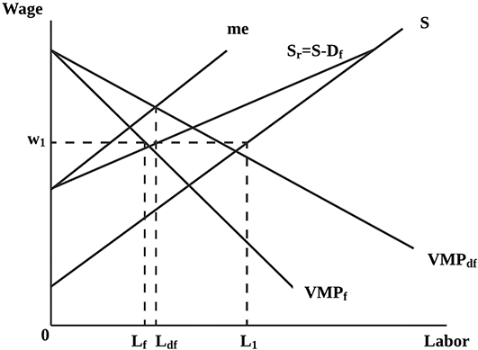
Figure 2.4 Profit maximization by a dominant employer

The profit maximizing behavior of the dominant employer leads to the same sort of allocative inefficiency that results from pure monopsony. Since the value of the marginal product exceeds the wage, the value created by employing one more unit of labor exceeds the social cost of doing so. Consequently, dominant employer behavior leads to a deadweight social welfare loss analogous to that of pure monopsony. The deleterious effects of the dominant employer’s profit maximizing conduct are muted, but not eliminated, by the competitive fringe employers. The more important the fringe’s presence in the labor market, the smaller will be the reduction in wages, employment, and social welfare.

2.6 Oligopsony

When there are several large employers in the labor market, the market structure is referred to as oligopsony. Individual efforts to depress the wage paid by restricting employment may be impaired by the conduct of the employer’s rivals. This market structure is a bit perplexing. Unlike the pure monopsony and its dominant employer variant, oligopsony may yield quite different outcomes. At one extreme, we may observe the pure monopsony solution, while the perfectly competitive solution may emerge at the other extreme. This range of outcomes is dismaying because it makes prediction quite difficult and, therefore, muddles antitrust policy.

2.7 Measuring Monopsony Power

Monopsony power is the ability of a large employer to influence wages by adjusting its employment level. In essence, the monopsonist recognizes that the supply function is positively sloped and that it can slide along that supply curve to a lower wage by decreasing its employment. This is why the monopsony wage deviates from the competitive wage. A measure of monopsony power should reflect this deviation. One way to do this is to adapt the Lerner Index of monopoly power to the case of monopsony.Footnote ²⁷

2.7.1 Lerner Index of Monopsony Power

Following Lerner, we define the monopsony power index as the VMP_L – wage gap relative to the wage paid:Footnote ²⁸

$\lambda =\frac{VM{P}_L-w}{w}.$

In Appendix A2.2, we show that the Lerner Index is the reciprocal of the elasticity of supply of labor:

$\lambda =\frac{1}{{\epsilon }_L}.$

Since the elasticity of the labor supply measures the responsiveness of the labor services supplied to changes in the wage, this is an appealing result. The more elastic the supply, the greater is the reduction in employment necessary to achieve any specific wage reduction. The effect of ${\epsilon }_L$ on $\lambda$ can be seen in several numerical examples, which are illustrated in Table 2.1 below.

Table 2.1 The effect of elasticity on the Lerner Index

${\epsilon }_L$	0.5	1.0	2.0	5.0	$\infty$
λ	2.0	1.0	0.5	0.2	0

Thus, when supply is inelastic (${\epsilon }_L$ = 0.5), there is a substantial deviation from the competitive result (200%). But the more elastic the supply, the smaller the deviation. In the limit, when ${\epsilon }_L=\infty$, the buyer is essentially in a competitive market and the deviation is zero.

2.8 Concluding Remarks

There is nothing good about monopsony in the labor market. The exercise of monopsony power leads to a social welfare loss because employment is suboptimal – too few labor services are being employed. This means that too little output is being produced. The economic results are unfortunately lower wages, reduced employment, higher output prices, consumer welfare losses, and a redistribution of wealth from employees to employers. The employer is the only winner. Everyone else loses.