

3.1 Introduction
Ever since it started to look as if the dinosaurs were done in by a nagging case of asteroids, the hypothesis has been pursued that every mass extinction has had an extraterrestrial cause, while some have expressed a strong preference for an earthly cause.Footnote 1 Here I frame the pursuit of the Nemesis hypothesis of an extraterrestrially caused periodicity in mass-extinction events as a process of ‘reading’ the fossil and geologic records in pursuit of narrative closure.Footnote 2 In the case of mass extinction, I am particularly keen on understanding how periodicity guides the search for evidence in pursuit of a causal narrative. In contrast to narratives of periodic extinction stand narratives of particular mass extinctions, where the plot is driven by the specific setting, characters, and one-off events. Of course, narratives of periodicity and one-time events do not exhaust the space of possible narrative explanations, and in the end I will describe somewhat of a middle path that seems to be gaining traction.
3.2 Periodicity of Mass Extinctions
In 1979, in Gubbio, Italy, a team of researchers led by Walter Alvarez discovered an iridium anomaly in sedimentary strata dated to be of end-Cretaceous age. This worldwide temporal horizon happens to coincide with the last known fossil occurrence of a number of biological taxa, including non-avian dinosaurs, ammonites, rudist bivalves, pterosaurs, mosasaurs and large numbers of plant and bird species. In terms of severity, the Cretaceous-Tertiary (or K-T) extinction (now known as the Cretaceous-Paleogene, or K-Pg extinction) ranks among the ‘big five’ mass extinctions in the fossil record: the end-Ordovician, Devonian, Permian, Triassic and K-Pg.
Like many discoveries in the earth sciences, the discovery of the iridium anomaly was serendipitous (Reference Glen and HookGlen 2002). The Alvarez team, assuming a statistically constant rain of meteoritic iridium throughout geologic time, thought that they could use that iridium flux to estimate elapsed time represented by sedimentary deposits. But the concentration they found was far off-scale relative to the known rate, and further lab analysis of samples confirmed that there was a ‘spike’ in iridium in a red boundary clay layer at the top of Cretaceous strata. Iridium concentrations in strata immediately above and below that layer fell off exponentially to zero (Reference Alvarez, Alvarez, Asaro and MichelAlvarez et al. 1980). Because Iridium is quite rare in the earth’s crust, the Alvarez team hypothesized an asteroid or comet impact.Footnote 3
Meanwhile, as the Alvarez group pursued evidence for an asteroid or other bolide impact at the Cretaceous–Tertiary boundary, David Raup and Jack Sepkoski were independently at work analysing broad extinction patterns in a synoptic database compiled by Sepkoski, A Compendium of Fossil Marine Families (Reference Sepkoski1982). Sepkoski had been compiling this database for years by combing the published literature for new reports of fossil occurrences, and continually updated this record of the first known and last known fossil appearances of marine families.Footnote 4 By tabulating the record of first and last appearances, a diversity curve for the entire Phanerozoic eon could be generated, and the number of families becoming extinct could be chronicled for each subdivision of geologic time. By Reference Raup and Sepkoski1982, Raup and Sepkoski’s statistical analyses of Sepkoski’s data resulted in a clear pattern of five large mass-extinction events – the so-called ‘big five’ – standing as outliers against a backdrop of smaller events (see Figure 3.1).

Figure 3.1 The ‘big five’ mass extinctions
The Ashgillian event at the close of the Ordovician, the Frasnian-Famennian event of the late Devonian, the Guadalupian-Dzhulfian event at the end of the Permian, the Norian event of the late Triassic and the Maestrichtian event at the Cretaceous–Tertiary boundary.
As Jack Sepkoski continued to compile a pen-and-ink database of first and last fossil appearance of marine families, his colleague at Chicago, David Raup, became interested in computerizing, tabulating, plotting and analysing them statistically. Whereas Sepkoski had plotted the data at the level of the stratigraphic series (e.g., upper Cretaceous), Raup decided to plot the data at a finer resolution, that of the stratigraphic stage (e.g., the Maestrichtian stage, a subdivision of the upper Cretaceous; Reference Sepkoski and GlenSepkoski Jr 1994). The gestalt they perceived was one of mass extinctions evenly spaced (Figure 3.2). Could this be a periodic array?
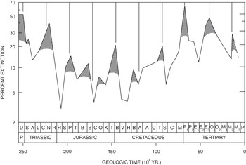
Figure 3.2 Graph of percentage extinction of fossil marine families for each geologic stage of the past 250 million years
With best-fit 26 million-year periodicity.
The stratigraphic record of the twelve largest mass-extinction events of the past 250 million years appeared to be periodic. However, two methodological constraints on the system had the potential to make the fossil record of mass extinction look periodic, regardless of whether it was or not. First, the stratigraphic record is divided into 40 stratigraphic stages (bins) of varying duration, and the dates of mass extinctions are resolved only to the level of the stratigraphic stage. Second, extinction peaks can only be recognized if they occur in non-consecutive stages, imposing some minimum separation between events. Spurious periodicity needed to be distinguished from the real thing. The questions raised were, within these methodological constraints: (1) what periodicity best fit the data? and (2) what is the probability of obtaining such a well-fitting periodicity simply due to chance?
To answer the first question, they needed to determine the best-fit periodicity, which required a measure of goodness of fit. Reference Raup and SepkoskiRaup and Sepkoski (1984) tried a range of periods from 12 million to 60 million years. For each period length they took a perfectly periodic time series and lined it up as closely as possible to the time series of mass extinctions and computed the standard deviation as a goodness-of-fit statistic. The best-fitting period came out to be 26 million years, with some standard deviation (call it sd*) from perfect periodicity. To answer the second question, they asked how frequently such a close fit to periodicity would occur if the timescale were randomized and extinction peaks were assigned to non-adjacent stages. As it turns out, the probability of obtaining a fit of sd* or better by chance was vanishingly small, and on this basis Reference Raup and SepkoskiRaup and Sepkoski (1984) were able to argue that the periodicity of 26 million years is very unlikely to have arisen by chance and thus should be provisionally accepted.Footnote 5
3.3 The Nemesis Affair and Narrative Closure
Raup and Sepkoski’s finding of periodicity, coupled with the Alvarez group’s discovery of an iridium anomaly coinciding with the mass extinction of the dinosaurs at the end of the Cretaceous period, led to the formulation of the Nemesis hypothesis (Reference Davis, Hut and MullerDavis, Hut and Muller 1984; Reference Whitmire and JacksonWhitmire and Jackson 1984). According to the Nemesis hypothesis, the sun has a companion star, Nemesis, which every 26 million years perturbs the orbits of comets in the Oort cloud, sending some of them on an earth-crossing orbit, with the resulting impact causing a mass extinction.Footnote 6 Linking periodicity with a possible extraterrestrial cause for mass extinction altered the temporality governing palaeontological research to one based on periodicity. In addition, it set in motion a search for a cause capable of producing the extinction periodicity: an astronomical search for a companion star (Reference MullerMuller 1988), a statistical search for periodicity in the ages of impact craters on earth (Reference Rampino and StothersRampino and Stothers 1984b) and a search for indicators of impact at stratigraphic horizons corresponding with mass extinctions around the world (e.g., Reference Claeys, Casier and MargolisClaeys, Casier and Margolis 1992). In short, this new ‘narrative of nature’ was compelling enough to galvanize a coalition of researchers from different disciplines, and changed the nature of extinction research, setting in motion a search for narrative closure.Footnote 7 Yet alongside the search, critiques were mounted, falling into one of five categories: general scepticism about the warrant for extraterrestrial causation (e.g., Reference HoffmanHoffman 1989), uncertainties in the ages of the dated events (e.g., Reference Grieve, Sharpton, Goodacre and GarvinGrieve et al. 1985), mismatch between timing of cause and effect, the possibility that periodicity may be spurious (e.g., Reference Stigler and WagnerStigler and Wagner 1987) and alternative explanations for the presence of the indicator in question (e.g., Reference Wang, Attrep and OrthWang, Attrep and Orth 1993).
3.4 Mass Extinction as a Recurring Narrative
While it was already accepted prior to Raup and Sepkoski’s finding of periodicity that there have been major mass extinctions in the history of life, there had been no reason to suspect that each of these mass extinctions had the same cause.Footnote 8 There was every reason to believe that if each mass extinction were to yield to any analysis at all, if the cause or causes were to be found, an idiographic approach was called for. Geologists and palaeontologists are highly trained in the identification of traces, in extracting information from remains, in inferring causal sequence, in arriving at consiliences of inductions and in pursuing multiple working hypotheses. In short, they are trained in reconstructing events from their available traces.Footnote 9 This may explain why, among many palaeontologists, the Nemesis hypothesis was met with suspicion. One eminent palaeontologist, Steven Stanley of Johns Hopkins, who in his 1987 book Extinction mounted a compelling argument that mass extinction is largely explicable in terms of well-documented changes in climate, summed up the prevailing view well:
If every peak forms part of the periodic array, then it must be attributed to the periodic agent. […] Do we really need to invoke an extraterrestrial cause for the event that occurred during the latter part of the Eocene Epoch, for example, when we know that at this time both deep-sea waters and terrestrial climates became cold (and remained so to the present) – and when we have a potential earthly explanation for these events in the form of the isolation of Antarctica over the South Pole via the final fragmentation of a large segment of Gondwanaland?Footnote 10
This is a paradigmatic idiographic narrative explanation. Stanley is pointing out that the elements of a narrative explanation were beginning to coalesce – approaching narrative closure – when out of nowhere, like an asteroid, comes a new narrative. Note that he is not contesting the plausibility or empirical support for the extraterrestrial narrative (although he would do so elsewhere), but rather whether, given the existence of a climatological narrative, the extraterrestrial narrative was necessary.Footnote 11
3.5 On Rereading the Book of Nature
Historian David Sepkoski has written an account of the rise of analytical palaeobiology entitled Rereading the Fossil Record, focusing on the period from around 1970 to the mid-eighties. Darwin and Lyell are understood to have brought us the metaphor of the fossil record as a book from which are missing several chapters, and from the remaining chapters many pages, and from the remaining pages many words, written in a slowly changing language.Footnote 12 Sepkoski’s account describes three historical phases of rereading that fossil record: literal, idealized and generalized. The literal rereading of the fossil record is exemplified by Reference Eldredge, Gould and SchopfEldredge and Gould’s (1972) model of punctuated equilibria in which the absence of morphological intermediates from the fossil record is not absence of evidence so much as evidence of absence (of morphologic change in species)! The idealized rereading is exemplified by the nomothetic palaeobiology of the Marine Biological Laboratory (MBL) group, which abstracted away from species as individuals and modelled them as particles in space and time, nomothetism denoting the search for lawlike generalities among historical events.Footnote 13 The generalized rereading combines empirical and statistical analysis made possible by the painstaking compilation and digitization of taxonomic data by Sepkoski’s father, Jack, with mathematical modelling undertaken for the most part with David Raup (Reference SepkoskiSepkoski 2012). During the generalized rereading phase of the rise of analytical palaeobiology emerged David Raup and Jack Sepkoski’s work on mass extinctions, first as a statistical phenomenon quantitatively distinct from background extinctions and then as a recurring phenomenon registering a 26 million-year periodicity.
In coming to a better understanding of how scientists reread the fossil record, it may be helpful or at least instructive to appeal explicitly to narrative theory as it has been developed in the study of literature. Clearly this is a vast field encompassing a large body of scholarship. I would like to start with the key distinction in narrative theory, as formulated by the Russian formalists, Vladimir Propp (1895–1970) and Viktor Shklovsky (1893–1984).Footnote 14
This is the distinction between the supposed chronological sequence of events, referred to as the fabula, and the way they are presented in the narrative discourse, the syuzhet. Notably, fabula and the syuzhet register different orderings.Footnote 15 The relationship between these two orderings of events contributes to the literary characteristics of a narrative, allowing for it to exert its effects on a reader, and to elicit a certain aesthetic response. For example, in Dostoevsky’s Crime and Punishment, Raskolnikov’s murder of the pawnbroker is presented early in the narrative. It is only after reading for a good number of pages that we learn from Porfiry Petrovich’s cross-examination that several months prior to the murder Raskolnikov had written an essay arguing that the extraordinary man is not bound by common morality. This ordering of the presentation of events between fabula and syuzhet elicits an affective response from the reader, for example a feeling of suspense over whether Raskolnikov will crack under questioning.
Crime and Punishment is rather noteworthy for its subversion of the narrative of a typical murder mystery, so, although it illustrates the difference between fabula and syuzhet, we might be better served using the more conventional genre of the ‘whodunnit’. In this genre, the murder is revealed early on in the syuzhet, and suspense builds until the identity of the murderer is eventually revealed. I will return to this idea later.
If we take the idea of reading (or rereading) the fossil record seriously, we might regard the traces in the fossil record as forming the syuzhet, from which the palaeobiologist infers the fabula. The palaeobiologist ‘reads on’, and keeps rereading in a search for narrative closure. If this is so, then the narrative structure of the mass-extinction account may help explain the search for evidence as the search for closure.
It is important to acknowledge disanalogies between narrative closure in reading a work of fiction and in reading the fossil record. From the reader’s point of view, in a work of fiction, the fabula is something inferred, and, depending on the work in question, there may not be sufficient textual evidence to adjudicate among rival fabulae. At first it might be tempting to think that something analogous is at work in reading the fossil record. Due to underdetermination, scientists may differ in their readings of the fossil evidence, with each reading consistent with the available evidence. In both cases, one might bring in background knowledge, theories of interpretation and the like to provide support for one reading over another. In both cases, we may have no choice but to sit pat with the situation unresolved. Yet there are at least two important disanalogies between reading a work of fiction and reading the fossil record. The first stems from the nature of fiction. It is entirely possible that an author is, to put it glibly, ‘all syuzhet and no fabula’. That is to say, there need not even exist an underlying fabula to which the syuzhet refers.Footnote 16 The author may present, in whatever order, a set of events in the narrative discourse over which there could be great disagreement as to what their true chronological ordering was, and it is possible that there does not even exist any true chronological ordering: what we have are the words on the page and an argument in favour of one reading or another. Indeed, Reference WalshWalsh (2001) has argued that even in conventional cases of narrative fiction, fabula is not ontologically prior to syuzhet. Rather, from the syuzhet, the reader is constructing – not reconstructing – a fabula (not the fabula) in an ongoing process of interpretation. Fabula is the reader’s working version of what happened in the world of the characters – a fictional world. Yet reading the fossil record differs from this: the history of life is not a fiction. First, the palaeontologist presumes that, whether it is empirically ascertainable, there does exist an ordering of events, wie es eigentlich gewesen, to which the syuzhet (the fossil record as it is read) must in some way be connected. The fabula of the history of life is ontologically (and temporally) prior to the syuzhet (order of presentation in the fossil record that the palaeontologist is reading). It is being reconstructed from the record it has left behind.Footnote 17 Second, the form of reading on which the palaeontologist is embarked allows her to expand the text, to look to other stratigraphic horizons, to seek out new evidence, to read on in search of narrative closure an ever-expanding text, in which one narrative is better supported than others, at which point narrative closure will have been achieved, at least temporarily. This is not to say that the situation is completely unlike that of rereading a work of literature, in which other information external to the text (e.g., early drafts, memoirs by the author, inter- and extratextual references, theories of interpretation) may help to support both the existence of a fabula and give some notion of what it is. Indeed, in the historical sciences in general, it has been argued that at any given time, even in the face of a fixed set of fossils and geological evidence (analogous to the closed form of the written text), the totality of the rest of science (theory, method, observations), which is constantly changing, enables an assessment of which of many possible fabulae are best supported (Reference JeffaresJeffares 2010).
Under periodicity, which presented a narrative of recurrent, extraterrestrial perturbation of the biosphere, the search for evidence looked completely different. Planetary geologists and astronomers began to reread the record of impact structures (craters, astroblemes) for evidence of periodicity (Reference Grieve, Sharpton, Goodacre and GarvinGrieve et al. 1985). While this record is even more fragmentary and less well-dated then the fossil record, it eventually did yield periodicity (Reference Rampino and StothersRampino and Stothers 1984a; Reference Rampino and Stothers1984b), and the hypothesis of impact periodicity continues to be pursued (Reference Rampino, Caldeira, Prokoph, Koeberl and BiceRampino, Caldeira and Prokoph 2019; Reference Rampino, Caldeira and ZhuRampino, Caldeira and Zhu 2020). At stratigraphic boundaries marking extinction events, iridium anomalies were sought and sometimes detected (although for certain events, such as the end-Permian extinction, iridium anomalies have so far turned out to be spurious; Reference ErwinErwin 2015 and personal communication). Where iridium anomalies proved wanting, other markers of impact were sought: shocked quartz (with a distinctive crystalline lattice), microtektites (bits of molten rock associated with the high heat of impact), buckminsterfullerenes, osmium isotopes and soot (Reference RaupRaup 1986: 75–87). Markers of one type or another proved adequate to justify continued pursuit of the hypothesis. Meanwhile, astrophysicists, chiefly Berkeley astrophysicist Richard A. Muller, continued to scan the heavens searching for Nemesis, which as of 2007 was still an ongoing search. The pursuit of narrative closure does not always end in achieving it.
To summarize, emplotting all mass extinctions of the past 250 million years in the narrative of a cause that recurs with clocklike regularity enabled Raup and Sepkoski to resurrect the nomothetism of the 1970s in which they had been integrally involved by fitting a periodic model to the record of mass extinctions, yet at the same time to create a narrative, a narrative of recurrence which drove scientists from a number of different fields – astronomy, planetary geology, isotope geochemistry, mineralogy and palaeontology – to embark on a quest for narrative closure on the basis of a periodic pattern or cause.
In so doing, Raup and Sepkoski’s research on extinction resolved an ongoing tension in the history of the earth sciences between uniformitarianism and catastrophism by putting forward an exemplar of a catastrophe (asteroid impact) that behaved according to a uniform periodicity rooted in the regularity of astronomical orbits. The Nemesis hypothesis was thus idiographic and nomothetic, catastrophist and uniformitarian, and it was a narrative explanation.
3.6 Rereading the Book of Nature through Diagrams
One step along the way to constructing a narrative of extinction is to ‘read’ and reread the stratigraphic record. In order to test whether patterns in the fossil record are consistent with a given causal narrative, such as sudden, catastrophic extinction, it is helpful to be able to investigate historical counterfactuals, which are narratives of events that could have happened, but did not. In the study of mass extinction, one of the templates for the formulation and articulation of counterfactual narratives has been the stratigraphic diagram. Stratigraphic diagrams do not operate alone to produce these counterfactual narratives, but in the context of tacit knowledge and ‘ways of seeing’ that are an extension of the practices of palaeontological and geological fieldwork. A common visual language and sets of practices makes possible the diagrammatic narratives that have been central to studies of mass extinction.
The stratigraphic diagram thus becomes a template for framing narratives of extinction and even for experimenting with alternative, counterfactual narratives; from reading through different configurations of syuzhet, scientists gain a sense of which fabulae are consistent with it, answering questions thrown up by the Nemesis hypothesis.Footnote 18
For example, in his 1989 paper, ‘The Case for Extraterrestrial Causes of Extinction,’ David Raup presents a diagram, plotting the distribution of fossil occurrences of different ammonite species in a stratigraphic section of late Cretaceous age in Zumaya, Spain, based on the fieldwork of Peter Ward (Figure 3.3). Ammonites, cephalopods with a coiled morphology, are one of the taxa that became extinct at the K-Pg boundary. The question Raup sets out to answer is whether this extinction was gradual, stepwise or sudden. Here one must distinguish between apparent and actual patterns: the apparent pattern of last known fossils and the actual pattern of last surviving members of the species. If the actual pattern of ammonite extinction (and, by extension, the end-Cretaceous extinction of other species) was gradual leading up to the K-Pg boundary, then a sudden cause such as a bolide impact is not tenable. If the actual pattern of extinction was stepwise, then a multi-phase event such as a comet shower is not ruled out. And if the actual pattern of extinction was sudden, then an impact-caused extinction becomes viable.
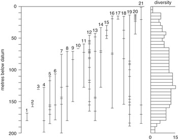
Figure 3.3 Stratigraphic ranges of 21 lineages (i.e., species genus Linnaeus) of ammonites found at Zumaya, Spain
Vertical scale marks distance in metres below the Cretaceous-Tertiary (today called the Cretaceous-Paleogene) boundary. Numbered vertical lines refer to ammonite lineages. Each horizontal tick mark designates a horizon at which a specimen of the lineage was found and identified. Note the ‘gappiness’ of the fossil records of the various lineages. For example, specimens of lineage 4 (Pachydictus epiplectus) were found and identified at 3 horizons: 200 m, 180 m, and 135 m below the Cretaceous–Tertiary boundary). The histogram on the right plots the number of lineages (inferred from first and last occurrences of specimens) in each 5 m interval (e.g., the 15 lineages who range through the 130 m to 125 m interval). Based on field data of Peter Ward.
The methodological problem palaeontologists face is that of stratigraphic range truncation: due to gaps in preservation or failure to find or identify species, there is often elapsed time between the last appearance datum (LAD) for any given species in the fossil record and the time that the species actually went extinct, a mismatch between apparent and actual patterns of extinction. This is a missing data problem. The consequence is that the fossil record of sudden, simultaneous extinction of many species can look as if the event were smeared out over geologic time: a sudden extinction event in the fabula will appear in the syuzhet as gradual, a phenomenon known as the Signor-Lipps effect (Reference RaupRaup 1986). Conversely, if there is a large hiatus in preservation or sampling, then a gradual extinction in which species became extinct one after another over an extended period of time will leave a record that looks as if species all became extinct simultaneously: a gradual extinction on the level of fabula will be read as sudden in the syuzhet. Alternatively, smaller hiatuses in preservation or sampling can mean an extinction is read as if it happened in a series of bursts – stepwise extinction – even if the extinction was gradual or sudden.
Reference RaupRaup (1989) points out a paradox in how palaeontologists have tended to read the fossil record. On one hand, palaeontologists know that the fossil record is gappy: absence of evidence does not (generally) constitute evidence of absence; the syuzhet requires interpretation in order to reconstruct the fabula. On the other hand, there is a tendency to read the last appearance datum as the time of extinction for a species. Raup believes this to be fundamentally a methodological problem, ultimately to yield to a quantitative treatment, but chooses to illustrate the point using an experiment – a thought experiment – which happens to take the form of a visual, counterfactual narrative. Suppose, he asks, that all fossil occurrences of ammonites were eliminated beginning at a stratigraphic horizon 100 m below the K-T boundary: what would the fossil record of this sudden mass extinction look like? As can be seen from Figure 3.3, he argues, it would look gradual (with a spurious step introduced at the 125 m mark).
As has been pointed out elsewhere, palaeontology has a distinctive visual culture that places a premium on being able to show visually that which might also be demonstrated analytically or mathematically (Reference Huss, Sepkoski and RuseHuss 2009). For example, when a palaeontologist looks at a stratigraphic diagram, he or she can visualize it as an idealized, synoptic representation of a rock outcrop embedded with specimens of fossil species, as well as the fruit of a great deal of integrative inference. It will be second nature for any geologist or palaeontologist to read this diagram from bottom (oldest) to top (youngest). Field skills and geologic training allow the interpreter to give the diagram a spatiotemporal reality that may not be perspicuous to others (Reference Huss, Bouton and HunemanHuss 2017). Embedded in such a diagram as that depicted in Figure 3.3 is a ‘research narrative’, as well as one of nature. Palaeontological field workers sought, found and identified fossils at certain horizons in the stratigraphic record. Tectonic forces may have distorted, tilted or completely inverted the sequence as found in the field. All is righted in the diagram. Laterally dispersed localities needed to be correlated using principles of stratigraphic inference to determine whether specimens of different species were found at the ‘same’ horizon. There are many such sketches of the reconstructive aspect of palaeontology that are encoded in a scientific diagram. While they need not be fleshed out each time, and the identities of those making the scientific contribution would itself need to be reconstructed from other sources, when palaeontologists look at a stratigraphic diagram they see encoded in it a community’s research narrative.Footnote 19
Yet Figure 3.3 also encodes a ‘narrative of nature’. Beds of sediment were laid down, organisms lived and died and left fossilizable hard parts. Periods of erosion or depositional hiatus, along with dissolution of shells, create gaps in the rock and fossil records. Narratives of morphological change and differentiation – microevolution and macroevolution – leave their traces in the patterns of fossil occurrences. Broad temporal trends in species gain and species loss, ultimately culminating in extinction, can be inferred from the patterns of diversity that are depicted in the running histogram jutting out from the right-hand side of the diagram. Tacit knowledge would enable most palaeontologists to provide a narrative sketch of what they see in Figure 3.3. Experts on ammonites may be able to venture a richer narrative, but some elements of the causal story remain outstanding. While scientists broadly understand some of the processes that gave rise to the patterns of spatiotemporal distribution of fossils in this diagram, ultimately, the causal analysis of evolution and extinction will need to be found elsewhere. The patterns in Figure 3.3 are the explanandum. Specific causal hypotheses are the explanans.
Figure 3.4 enables a visual reading of a counterfactual narrative: given the same evolutionary history and gappy stratigraphic distribution of fossils, what would the pattern of last appearances look like if extinction occurred suddenly at the 100 metre datum?Footnote 20 Because the temporal sequence of geological and evolutionary events leaves a spatial record – a vertical array of fossil occurrences organized into geologic strata consisting of depositional, erosional and quiescent horizons – the resulting visual chronology lends itself to a narrative treatment, including the formulation of alternative narratives to help assess the plausibility of the proposed narrative explanation under consideration. In the same fashion as Figure 3.3, the thought experiment depicted in Figure 3.4 draws upon the knowledge and interpretive habits of palaeontologists, who are now in a position to see that even cases of sudden, simultaneous extinction can leave a misleadingly gradual trace in the fossil record.
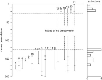
Figure 3.4 Thought experiment on causes of extinction
Here a thought experiment is posed: what if all lineages had suddenly become extinct at a datum 100 m below the Cretaceous-Tertiary boundary? Would the pattern of last appearances look sudden or gradual? Note that despite the instantaneousness of this hypothetical extinction event, the apparent pattern of die-off is gradual, with a spurious ‘step’ appearing at around the 125 m mark. The conclusion may be drawn that an extinction event that was in fact sudden and simultaneous may look gradual when filtered through the ‘gappiness’ of the fossil record. From data plotted in Figure 3.3.
In the historical sciences, one often wishes to reconstruct what happened – to produce a historical narrative – based on physical traces, background theory and other assumptions.Footnote 21 One way to assess a pattern of physical traces as evidence for or against a proposed narrative is to ask whether a similar pattern would have been expected under an alternative narrative scenario. In these diagrams, the focal question is not what caused the extinction, but how to read the fossil record – what combination of species extinction and spotty preservation does it reflect? Understanding their relative contributions can give rise to a corrected pattern of species extinction, which is what, qua historians of life, palaeontologists seek to explain.
Ultimately, however, the narrative that explains the fossil record as we find it, that gives an account of the patterns therein, is relevant to the grander, causal narratives of mass extinction: extraterrestrial, climatological, ecological, volcanogenic, etc. At a minimum, the fossil patterns must be consistent with the proposed mechanism of extinction, but the search for additional evidence – of impact, climate change, trophic shift or volcanism – has taken scientists beyond the fossil patterns themselves to competing narratives of extinction and the evidence relevant to adjudicating among them.
3.7 Narrative Closure in Philosophical Context
Philosophers have disagreed about the epistemic underpinnings of narrative closure in the historical sciences. For starters, there remains the very real possibility that, depending on the question at issue, narrative reconstructions of the past are always one data point or a few data points away from being reopened such that scientists should always be open to the temporariness of narrative closure (Reference TurnerTurner 2007). To this, I should add that narrative explanation is remarkably flexible and resilient in the way that components can be retained as well-established (e.g., suddenness of extinction, periodicity), even as evidence for other components of the narrative is found lacking, inconclusive or is even overturned (e.g., evidence for the existence of Nemesis). Second, there is an ongoing debate about what epistemically grounds narrative closure (Reference ClelandCleland 2002; Reference TurnerTurner 2007; Reference Forber and GriffithForber and Griffith 2011). Cleland has argued that narrative closure is achieved when a ‘smoking gun’ is found: a piece of evidence that is consistent with one narrative but inconsistent with its rivals. In this view, the Chicxulub crater that has been dated to the end of the Cretaceous period played this role in establishing an asteroid impact as the cause of the K-Pg extinction. Yet Forber and Griffith point out that any given datum only has evidentiary value against a background of auxiliary assumptions, which in the historical sciences can be difficult to test. Hence, data that appear to rule in one hypothesis and rule out its rivals may prove to be indecisive, because their doing so is too sensitive to weak auxiliary assumptions: there is no one-to-one mapping between fabula and syuzhet. As we saw earlier, in the discussion of Reference RaupRaup’s (1989) rereading of the stratigraphic record at Zumaya, evidence that the K-Pg extinction was gradual, based on a petering out of certain species as the K-Pg boundary is approached from below, can easily be shown to be consistent with sudden mass extinction if different assumptions are made about how preservation is expected to result in the observed fossil record. It is easy to ‘explain away’ inconsistencies in this way: one can ‘save the narrative’ by deflecting inconsistencies to auxiliary assumptions. Thus, Reference Forber and GriffithForber and Griffith (2011) have argued that a more promising and robust way to achieve closure that is likely to be less ephemeral is to ground historical inferences by a consilience of inductions (Reference WhewellWhewell 1858), namely by finding lines of evidence that each depend on independent sets of auxiliary assumptions. They give the example of several different sets of evidence that were used to predict the size of the asteroid impact at the end of the Cretaceous and the degree to which they did or did not share auxiliary assumptions as crucial factors in assessing the strength of evidence, both in probabilistic terms and in reception by scientists (Reference Forber and GriffithForber and Griffith 2011). For my purposes here, I merely wish to note that historical science as the pursuit of narrative closure is consistent with both of these models.
3.8 Conclusions
A recurrent narrative such as the Nemesis hypothesis challenges some distinctions that have been used to set up oppositions between approaches in palaeontology. Simply put, a narrative of lawlike recurrence has both nomothetic and idiographic components consisting of the mathematical laws governing the periodic forcing agent as well as the overall causal narrative explaining which taxa became extinct, which survived and why. It also challenges the distinction between uniformitarianism and catastrophism, in a sense rendering bolide impact uniformitarian – a periodic catastrophe, as it were (Reference Sepkoski and GlenSepkoski Jr 1994).
The narrative of recurrent extinction known as the Nemesis hypothesis set in motion a search for narrative closure, and for communities of scientists, a quest for evidence that each mass extinction had been caused by an extraterrestrial impact. In the case of the K-Pg extinction, in which the dinosaurs, ammonites and a number of other groups perished, narrative closure was achieved with the discovery of an impact crater of approximately the size predicted on the basis of the iridium anomalies found around the world (Reference Forber and GriffithForber and Griffith 2011). This effectively closed off debate about alternative narrative explanations for that particular extinction.
The legacy of the Nemesis affair is far more complicated. For starters, the periodic pattern in mass extinction appears to be too stable to be compatible with the instability of the calculated orbit of the supposed companion star Nemesis (Reference Melott and BambachMelott and Bambach 2010)! Still, the pursuit of closure in the impact narrative is ongoing, especially on the part of Michael Rampino and colleagues (Reference Rampino, Caldeira, Prokoph, Koeberl and BiceRampino, Caldeira and Prokoph 2019; Reference Rampino, Caldeira and ZhuRampino, Caldeira and Zhu 2020), but in general there is greater pluralism. Volcanism and deep ocean anoxia are among the proposed causal agents at horizons where evidence of impact is lacking (Reference Rampino, Caldeira, Prokoph, Koeberl and BiceRampino, Caldeira and Prokoph 2019), and three episodes of large-scale igneous province (LIP) eruptions are dated at times that coincide with the inferred ages of the three largest known impact craters, all of them falling at or near extinction peaks now computed as having a 27.5 million year periodicity (Reference Rampino, Caldeira and ZhuRampino, Caldeira and Zhu 2020). This periodicity has been found to be statistically significant over the past 500 million years, extending it twice as far back in time as had been found in Raup and Sepkoski’s original analyses (Reference BambachBambach 2017; see also Reference Erlykin, Harper, Sloan and WolfendaleErlykin et al. 2017). It is close to the half-period of passes of the solar system through the plane of the Milky Way galaxy – conjuring the image of a ‘Galactic Carousel’ (Reference Rampino, Haggerty, Rickman and ValtonenRampino and Haggerty 1996). In a bit of brand differentiation, the hypothesis that the concomitant mass-extinction periodicity is due to the resultant galactically governed influx of asteroids, comets or even dark matter has been dubbed the ‘Shiva hypothesis’ (Reference GouldGould 1984; Reference Rampino, Haggerty, Rickman and ValtonenRampino and Haggerty 1996). Statistical searches for periodicity in the timing of mass extinctions, asteroid crater ages and oscillations through the galactic plane have been ongoing (Reference Rampino and StothersRampino and Stothers 1984a; Reference Melott and BambachMelott and Bambach 2014; Reference Rampino, Caldeira, Prokoph, Koeberl and BiceRampino, Caldeira and Prokoph 2019; Reference Rampino, Caldeira and ZhuRampino, Caldeira and Zhu 2020). These analyses have also turned up an approximately 60-million-year periodicity in an isotopic signature in marine sediments that has given rise to a variety of alternative narratives involving internal drivers of plate tectonic activity, galactically driven increases in the influx of cosmic rays with effects on upper atmospheric ionization and climate and possible coupling between astronomical cycles and internal geodynamical cycles (Reference Melott, Bambach, Petersen and McArthurMelott et al. 2012).
In other words, despite the pursuit of narrative closure, the science does not seem to be approaching it. Rather, narrative seems to be a rather flexible tool for adjusting to what scientists find as they ‘read on’. So what does the Nemesis affair teach us about the pursuit of narrative closure in the case of periodicity of mass extinction? First, periodicity in the temporal pattern of the mass extinctions themselves has stood up to improved resolution of the data, revisions to the geological timescale (Reference Melott and BambachMelott and Bambach 2014) and the use of a range of different statistical methods (Reference Rampino, Caldeira and ZhuRampino, Caldeira and Zhu 2020). Closure seems to have been achieved in the pattern in the timing of the mass extinctions themselves. Second, as might be expected when vastly different narratives compete, such as ‘earth-bound’ narratives of particular mass extinctions and astronomically driven recurrent causes of the periodic pattern, attempts to achieve narrative closure in one camp are met with attempts to keep the narrative open in another, sometimes by folding the objections in to produce a unifying narrative (Reference Rampino, Caldeira and ZhuRampino, Caldeira and Zhu 2020). Third, the Nemesis narrative itself, while today finding few adherents, reoriented attitudes such that astronomical processes are deemed worthy candidates for driving biotic and geologic phenomena on planet Earth. Finally, in the case of periodic mass extinction, the search for narrative closure has been empirically and methodologically fruitful. Scientists really are pursuing narratives, seeking to assemble a causal story that can account for the apparent periodicity – we see this particularly in the attempt to connect galactic processes with oceanic, atmospheric and geological processes – drawing on that narrative to guide an empirical quest, and reading on in pursuit of evidence that can provide narrative closure, however elusive it may be.Footnote 22
4.1 Introduction
In an article entitled ‘The Geologist as Historian’, one of the twentieth century’s foremost British geologists, H. H. Read (1889–1970), characterized geology as ‘earth-history’ (Reference Read1952: 409). Read’s point was that geology has a lot in common with human history, dealing as it does with the reconstruction of particular events that occurred in the past, albeit on a very different timescale (and minus a role for human agency). Read noted that in geology, as with its counterpart in the humanities, ‘no event has ever been exactly repeated’ (Reference Read1952: 411). A possible point of contention emerges, however, when this analogy is extended to the mode of explanation in geology. It is uncontroversial to state that explanations in history have a narrative form, but suggesting that ultimately all explanations of events in time are narrative in structure (as asserted by Reference Richards, Nitecki and NiteckiRichards 1992: 22–23) may well cause unease among many geologists who do not wish their science to be associated with a term which may seem vague and unscientific, or which is suggestive of ‘mere’ storytelling.Footnote 1
In this chapter, I will seek to emphasize and uphold the narrative nature of geology, a property which may not be widely understood or appreciated, even by its own practitioners, but which has a logic and rigour of its own (Reference FrodemanFrodeman 1995: 966). Unlike those in human history, narratives in geology are always strictly bounded by what is possible according to the general laws of physics and chemistry; they are also tightly constrained by what is geologically plausible, although there is always scope for daring or ‘outrageous’ hypotheses (Reference DavisDavis 1926), which are open to review and testing by the geological community.
Without being too prescriptive, the essence of a narrative statement can be usefully thought of as specifying two time-separated events, so that the prior event is understood to have given rise to, and thereby to explain, the later event;Footnote 2 it is typically expressed in the past tense (Reference DantoDanto 1962: 146). More complex narratives, involving multiple events and processes which have interconnected causal relationships, are built on this simple formulation. A narrative explanation therefore specifies the causal connections in a temporal sequence of events or processes. It is important to note that a narrative in a historical science such as geology is neither a chronicle (a chronological listing of disconnected events),Footnote 3 nor is it a merely descriptive exercise. It has been argued that a defining characteristic of historical sciences such as geology is that they rely on narrative sentences for understanding (Reference GriesemerGriesemer 1996: 66). As will become apparent in the course of this chapter, however, narratives in the geological literature are not always explicitly narrative.
4.1.1 Narrative Reasoning
While the most obvious function of narratives in geology is to communicate explanations or interpretations, narrative is also fundamental to geological reasoning. Mary Morgan (Reference Morgan2017) describes the mental process of ‘narrative ordering’, in which what may initially appear to be disconnected events are able to be woven together into a coherent whole, thereby imparting meaning to them. Narrative ordering may take place in a variety of settings, such as in the act of individual reflection, in the course of writing or sketching, or in the process of discussion with others. The idea expounded by Morgan refers to common practice in the social sciences, but it describes well the route a geologist might follow in order to make sense of a collection of puzzling observations. Interpreted events in geology also derive their meaning from being part of an overall story; that is, they only make sense when they contribute to and form a component of an overarching narrative. The theory of plate tectonics, involving the separation and collision of continents on a timescale of hundreds of millions of years, supplies the most obvious ‘big picture’ narrative in modern geology.Footnote 4 Robert Frodeman refers to this property in which ‘details are made sense of in terms of the overall structure of a story’ as ‘narrative logic’ (Reference Frodeman1995: 963). However, the term ‘narrative logic’ could usefully be extended to include the criteria employed in narrative ordering. Hence, narrative logic can be understood as having both an internal dimension, through the coherent ordering of related events, and an external dimension, via the relationship of those events to overarching ideas.
Counterfactual reasoning can serve as another powerful device in the geologist’s mental toolbox, although it may not be explicit in many written accounts. Deliberately changing elements of a geological narrative or filling in gaps in the data to see what difference it makes to the overall picture can reveal flaws or strengths in a particular argument. Hence, counterfactual reasoning can help to expose narratives that do not make geological sense (i.e., do not display narrative logic), clearing the way for ones that do.Footnote 5
4.1.2 The Impermanence of Geological Narratives
The evidence available to the geologist seeking to piece together ‘the fantastic drama of the earth’s crust’ (Reference ReadRead 1952: 409) consists of tracesFootnote 6 of events which ceased long ago but which have been left behind in rocks, fossils and landscapes. These traces, however, are prone to concealment, degradation, even complete destruction over the vast expanse of geological time: weathering and erosion act on rocks at the surface, while at depth, profound changes may be wrought by pressure, heat or geochemical reactions. It is also true that while some traces are particularly susceptible to elimination, certain geological processes leave no traces at all (e.g., Reference Tipper, Smith, Bailey, Burgess and FraserTipper 2015). As Kleinhans, Buskes and de Regt (Reference Kleinhans, Buskes and de Regt2005: 290) conclude, a result of this incompleteness is that ‘theories and hypotheses [in geology] usually are underdetermined by the available evidence’. Consequently, the word interpretation tends be used more frequently than explanation in geology.Footnote 7 The two terms are almost synonymous, although interpretation suggests something more provisional and hypothetical.Footnote 8 In the context in which it is generally used by geologists, an interpretation can be understood as a response to the question ‘What caused these traces?’ (see, for example, Reference Faye, Su, rez, Dorato and RédeiFaye 2010: 108–111).
In a discipline in which previously concealed or overlooked traces have a habit of eventually turning up, new ideas, analytic techniques and interpretative methods are constantly being developed. Old theories are regularly replaced, so narratives tend to come with a degree of implied uncertainty and provisionality and are often not assumed to be the last word. When the evidence changes or when theories are superseded it is not unusual for geological narratives to be modified or even to be completely rewritten, although intellectual inertia might retard the process of revision.
4.1.3 Central Subjects in Historical Narratives
The construction of a historical narrative requires the identification of a central subject (Reference HullHull 1975). Its purpose is to provide the coherence necessary for intelligibility (Reference FrodemanFrodeman 1995: 965–966) and to form ‘the main strand around which the historical narrative is woven’, a key requirement being continuity in space and time (Reference HullHull 1975: 262). In the rest of this chapter, the role of central subject will be occupied by the outcrop of a particular stratum of ancient rock situated in Scotland. The changing historiography of this layer will serve to illustrate both the narrative nature of geology and the impermanent character of many geological narratives.Footnote 9 The focus of the case study is on how geologists communicate through papers and articles within the community of fellow practitioners.
4.2 The Case of the Stac Fada Member
The cliffs along the Assynt coastline of Sutherland, north-west Scotland, are formed of some of the oldest sedimentary rocks in the British Isles. The reddish-brown outcrop has been known informally as the Torridonian since the late nineteenth century when it was recognized to be of Pre-Cambrian age.Footnote 10 Despite their great antiquity, the rocks are acknowledged to be remarkably well preserved. They were originally assumed to be unfossiliferous, although eukaryotic microfossils are now known to be present (Reference Brasier, Culwick, Battison, Callow, Brasier, Brasier, McIlroy and McLoughlinBrasier et al. 2017).
Writing in 1897, J. G. Goodchild of the Geological Survey of Great Britain drew a direct analogy between the ancient sediments that formed the Torridonian rocks and the modern sands currently being deposited in ephemeral rivers and lakes in the Sinai Desert, on the basis of their remarkably similar form and composition:
To my mind one of the most striking and significant illustrations of the principle upon which geologists interpret the records of the Past, by the study of the Present, is to be found in the Torridonian areas of the North-West of Scotland. If we review the conditions obtaining in the Sinaitic Peninsular […] we find going on there to-day almost the exact counterpart of what must have taken place in Pre-Cambrian times in Sutherland and Ross.
The Geological Survey studied and mapped the rocks of north-west Scotland in a major campaign that ran from 1883 to 1897. The results were published in a substantial Memoir several years later (Reference Peach, Horne, Gunn and CloughPeach et al. 1907), in which descriptions of the Torridonian rocks occupied one of five subsections.
Following something of a hiatus during the early twentieth century, research on the Torridonian resumed in the 1960s. A research group was set up in the Geology Department of Reading University focused exclusively on furthering knowledge and understanding of the Torridonian (Reference StewartStewart 2002: 3). Initial reconnaissance work revealed the rocks to be ‘unexpectedly complex’ (Reference Gracie and StewartGracie and Stewart 1967: 182), and it took several years of careful fieldwork to unravel the stratigraphic relationships. Among the unexpected complexities encountered by the Reading group was a particular layer which was noted to be generally between 10 m and 30 m thick. In the redefinition of Torridonian stratigraphy undertaken by the Reading group, this layer was named the Stac Fada Member (Reference StewartStewart 2002: 5).Footnote 11 This rock unit, the outcrop of which stretches across more than 50 km of coastline (Figure 4.1), was regarded as unremarkable by the nineteenth-century Survey geologists,Footnote 12 but was noted by the Reading researchers to differ in a number of significant respects from the layers immediately above and below (Reference StewartStewart 2002: 9–11).
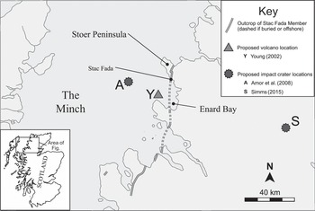
Figure 4.1 Location map of the Stac Fada outcrop
D. E. Lawson’s (1972) study of the Stac Fada Member described some of its constituents as angular shards of pumice, green particles of devitrified glassFootnote 13 and accretionary lapilliFootnote 14 (as shown in Figure 4.2). These were all interpreted as products of a nearby volcano. As with Goodchild’s Sinai Desert comparison, this interpretation was made by analogy with present-day processes. Accordingly, the Stac Fada Member was interpreted either as a pyroclastic flow – an airborne surge of fluidized ash and other fragments derived from a violent eruptive event (Lawson 1972) – or as more of a surface-bound volcanic mudflow (Reference StewartStewart 2002).

The volcanic interpretation of the Stac Fada Member initially seemed to fit the field observations well and it held sway for several decades. The absence of a volcanic vent in the surrounding landscape was not seen as problematic, given the long-term effects of erosion and burial. Based on the distance that present-day accretionary lapilli are known to travel through the air in an eruption, the volcanic vent was suggested to have lain a short distance offshore (Reference YoungYoung 2002: 7–8; point Y in Figure 4.1). However, it was apparent that there were some aspects that did not add up. For example, the lack of evidence for additional contemporaneous flows was regarded as ‘curious’ by Lawson: he explained that one ‘would not really expect volcanic activity to cease after a single eruption’ (Lawson 1972: 346, 360). Furthermore, several ‘thorny problems’ (Reference StewartStewart 2002: 10–11) were identified in the geological evidence. For instance, indicators of transport directions in the sediments showed that there had been an ‘abrupt change’ in the slope of the land from east to west ‘immediately prior to deposition of the Stac Fada Member’ (Reference StewartStewart 2002: 10–11). This was difficult to explain in terms of the volcanic hypothesis given that the outcrops along the coast were estimated to have been located too far from the putative volcano to have been affected by any associated land movements. Although several modes of volcanic emplacement had been proposed, it was concluded that none of them satisfactorily explained all of the field observations (Reference StewartStewart 2002: 10–11), and Stewart noted that, in 2002, the volcanic hypothesis remained ‘controversial’ (Reference StewartStewart 2002: 65). Despite these unresolved issues, the phenomenon of Stac Fada volcanism was incorporated, albeit with a degree of incongruity, into the body of literature on Scottish geology. For example, a major synthesis of the tectonic and magmatic evolution of Scotland included a short section on Stac Fada volcanism, in which the authors referred to it as ‘enigmatic’ (Reference Macdonald and FettesMacdonald and Fettes 2006: 232–233).
4.2.1 Old Evidence, New Discovery
Since 2004, the Torridonian outcrop has formed part of the North West Highlands Geopark and has become a popular destination for geology undergraduate field trips. On an Oxford University field course in 2006, postgraduate geologist Ken Amor was serving as an assistant to the teaching staff. Amor had recently returned from Ries in Bavaria where he had been studying the rocks around one of Europe’s few recognized meteorite craters. His attention was drawn to the distinctive green fragments of devitrified glass in the Stac Fada outcrop which had been highlighted by the Reading geologists. Although they were consistent with the prevailing volcanic interpretation, he had seen remarkably similar crystals close to the Ries crater, where they were interpreted to have been formed by the melting of the surface rocks in the impact event. There were no known instances of a major meteorite strike in the British Isles, but the green particles aroused Amor’s curiosity. A microscopic examination of thin sections of the rock in question would provide a test of Amor’s hunch, and on returning to Oxford he discovered that his department already held some thin sections that had been made from rocks collected on previous field trips.Footnote 15 However, he knew that the chances of finding anything new were not promising. ‘How many countless eyes of undergraduates had looked at these very same thin sections over several decades and not spotted anything unusual’?Footnote 16
What Amor hoped to see down his microscope were crystals of shocked quartz – a form of silica which bears the marks of the instantaneous application of stresses that are far higher than can occur in terrestrial processes, and which is regarded as an unequivocal indicator of a so-called ‘hypervelocity impact’. Against his expectations, Amor did find grains of shocked quartz in the Stac Fada thin sections (Figure 4.3), and the implications of his discovery soon dawned on him. He later reflected: ‘I remember thinking at the time that at that moment I was the only person […] to realise that the UK had been struck by an asteroid […] I didn’t tell my supervisor for two days because I wanted to hold on to that discovery moment for a little longer’.Footnote 17

Amor’s moment of insight has led to the Stac Fada Member being reinterpreted as an ejecta blanket – the material violently thrown out of the crater formed by the impact of a massive extraterrestrial body, overturning the previous interpretation of the layer as the product of a volcanic eruption and resolving many of the inconsistencies surrounding that explanation. For example, the sudden change in the slope of the land now made sense as a consequence of the impact. Amor published his findings in a co-authored paper two years after the breakthrough discovery (Reference Amor, Hesselbo, Porcelli, Thackrey and ParnellAmor et al. 2008). In addition to shocked quartz, the paper presented further evidence of an impact origin including the shocked form of another mineral (biotite) and key geochemical indicators such as anomalous chromium isotope values and elevated abundances of platinum group metals such as iridium. Subsequently, grains of shocked zircon were discovered in the Stac Fada deposit (Reference Reddy, Johnson, Fischer, Rickard and TaylorReddy et al. 2015), further confirming the impact ejecta interpretation. The melange of angular fragments and partially melted material in the Stac Fada Member is now routinely referred to as a suevite, the term for such a deposit created by an extraterrestrial impact.Footnote 18 The particles of devitrified glass and accretionary lapilli which had been assumed by the Reading geologists to be uniquely diagnostic of volcanic eruptions were evidently also capable of being formed in major meteorite impacts. This had been recognized from evidence at the Ries impact site for some time (Reference Kölbl-EbertKölbl-Ebert 2015: 275), a fact of which Amor would have been aware. According to radiometric dating of the Stac Fada Member, the impact occurred approximately 1.2 billion years ago, placing it in the Mesoproterozoic Era (Reference Parnell, Mark, Fallick, Boyce and ThackreyParnell et al. 2011).Footnote 19
There is no sign of the impact crater from which the Stac Fada Member was ejected. As with the now discarded volcanic interpretation and the absence of a volcano, this is not surprising given the burial or removal by erosion of much of the Torridonian outcrop in the last billion or more years. Different lines of reasoning by different geologists, but based essentially on the same evidence, have resulted in two different locations being posited for the crater (A and S in Figure 4.1). Amor et al. (Reference Amor, Hesselbo, Porcelli, Thackrey and Parnell2008; Reference Amor, Hesselbo, Porcelli and Price2019) suggest that a point in the Minch Basin 15–20 km to the north north-west of Enard Bay, an area that would have been dry land at the time of impact, is the most likely location, while an alternative hypothesis by Simms has the crater deeply buried onshore about 50 km to the east of the outcrops along the coast (Reference SimmsSimms 2015). Further data-gathering work in the form of expensive geophysical surveys or borehole drilling would be required to confirm or deny both proposals. However, Simms’s location has been criticized as being inconsistent with the overarching narrative of the plate tectonic history of northern Scotland (Reference Butler and AlsopButler and Alsop 2019: 443), and, in an example of counterfactual reasoning, Amor et al. Reference Amor, Hesselbo, Porcelli and Price(2019) argue against Simms’s location by pointing out that there would have been a topographic obstruction blocking the path of the ejecta blanket if it came from the east (Reference Amor, Hesselbo, Porcelli and PriceAmor et al. 2019: 842).
Three years after the publication of the discovery paper (Reference Amor, Hesselbo, Porcelli, Thackrey and ParnellAmor et al. 2008), volcanologists Michael Branney and Richard Brown addressed the question of exactly how the Stac Fada Member might have been emplaced. Nothing remotely approaching the scale of the meteorite impact from which the deposit is believed to have originated has ever been observed in recorded history,Footnote 20 and terrestrial impact ejecta blankets are commonly not well preserved, limiting the availability of possible analogues. The example at Ries is a notable exception, however, and Branney and Brown (Reference Branney and Brown2011) highlight parallels between the Stac Fada deposit and the Ries suevite. The absence of a crater, however, means that there is no way of investigating the relationship between it and the ejecta.
The authors note that while there are ‘important differences’ between the ejecta from impacts and those from volcanoes – for example, the presence of shocked minerals and distinctive geochemistry – there are also ‘striking similarities’ (Reference Branney and BrownBranney and Brown 2011: 287–288). The distinctive components of the Stac Fada deposit, including the presence of devitrified glass and accretionary lapilli, as well as the order in which they were deposited, resemble those ejected from large explosive volcanic eruptions. These similarities have led them to deduce that emplacement mechanisms comparable to pyroclastic processes associated with volcanoes were at work and they have coined the analogous term, impactoclastic (Reference Branney and BrownBranney and Brown 2011: 276) to describe their model, which details how the Stac Fada impact ejecta blanket could have been deposited (as we can see in Figure 4.4).
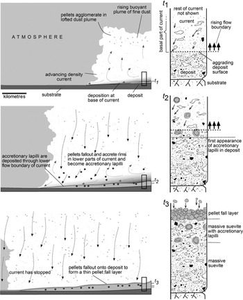
Figure 4.4 The impactoclastic emplacement of the Stac Fada ejecta blanket
For the benefit of the non-geologist reader, three pairs of images show the situation at successive points in time immediately following the meteorite impact. Each pair consists of a panel showing a cross-section through the dust plume thrown up by the impact (on the left) and a column representing the vertical accumulation of different types of debris deposited by the plume by that time (on the right). The time sequence, t1 to t3, runs from top to bottom. In the plume cross-sections, the crater lies out of frame to the right and the plume moves from right to left through the time sequence. Along the base of each of these cross-sections is the layer of debris deposited from the plume. This increases in thickness with time as marked by the ticks labelled t1, t2 and t3 at the bottom right of each cross-section. The location of each column of debris is marked by a rectangular outline in the bottom right of each corresponding plume cross-section. An understanding of how the overall diagram is put together, along with some technical (geological) knowledge, enables it to be read as a self-contained narrative.
4.3 Tracing the Narratives
4.3.1 Geological Narratives, Explicit and Implicit
At first glance, the writings of the geologists who have worked on the Torridonian outcrop since the late nineteenth century seem to contain few obvious instances of narrative statements of the kind discussed in the introduction, i.e., those which causally connect time-separated events. Notable instances include parts of Goodchild’s (Reference Goodchild1897) paper on the desert environment in which the Torridonian sediments were interpreted to have been deposited. For example, in the following passage he gives a straightforwardly narrative account of the weathering processes by which the Torridonian sands and shales would have been formed from the breakdown of pre-existing rocks based on observations made in the present-day Sinai environment:
[R]ain fell only occasionally, or practically never, and only on those occasions when thunderstorms happened to burst over the regions in question. At other times the arid conditions gave rise to great diurnal ranges of temperature. The rocks in consequence were heated soon after mid-day far above the temperature usual in more humid climates, and by early morning, owing to rapid radiation, had cooled down to the opposite extreme. In a rock composed of constituents of diverse mineral character differential expansion takes place, owing to their different coefficients of expansion. The felspars in the rocks […] gave way under the strain set up by extreme expansion and contraction, due to the rapid changes of temperature. The ferro-magnesian minerals […] in like manner splintered into fragments so small that they were easily blown away as dust by the wind. Little by little the rocks crumbled down, and of their wasted portions the larger part slid down the valley side as talus, to be eventually distributed and spread out in the bottoms of the wadies by the action of the occasional torrents arising during storms; the remainder, chiefly in the form of dust, was blown far and wide by the winds.
Another noteworthy narrative passage occurs as part of the impactoclastic model of Reference Branney and BrownBranney and Brown (2011). The following excerpt accompanies an explanatory ‘cartoon’ (the main part of which is reproduced here as Figure 4.4):
Time frames (t1–3) [depict] the generation and evolution of ash aggregates within an impactoclastic current. Turbulent entrainment of atmospheric air along the upper mixing zone of the current results in expansion and lofting, generating a buoyant dust plume. Within this [plume], ash pellets start to form (t1). Once these pellets become too large to be supported by turbulence in the lofted plume, they drop to lower parts of the current, dry out, accrete concentric ash rims (t2), and become deposited as fully formed accretionary lapilli, along with suevite from the base of the current. After cessation of the current, ash pellets fall out from the drifting buoyant dust plume and deposit directly on the top of the suevite (t3). The absence of accretionary lapilli in the lower parts of deposits is due to the time lag between the onset of deposition from the base of the current and the formation of pellets, their descent into the current, their growth within the current into accretionary lapilli, and their subsequent deposition.
The use of images to complement or clarify textual narratives is common in geology, and this text is designed to be read alongside the diagram. With appropriate geological knowledge and understanding of the context, however, the diagram itself could be read independently as a narrative, tracing as it does the temporal and spatial sequence of deposition caused by the transit of the waning dust plume.Footnote 21
In each of the passages by Goodchild (Reference Goodchild1897) and Branney and Brown (Reference Branney and Brown2011), the narrative structure of temporally arranged and causally connected sequences of events and processes is evident. Words and phrases denoting events and processes include ‘differential expansion’, ‘splintered into fragments’, ‘turbulent entrainment’ and ‘deposition’; while causal connections are signalled by ‘gave rise to’, ‘in consequence’, ‘results in’ and ‘generating’, among others. Both passages also illustrate the role of physical laws in constraining geological narratives. For example, Goodchild refers to the differential expansion of minerals when heated, and the effects of turbulence, expansion and gravity in a hot dust plume form part of the account of Reference Branney and BrownBranney and Brown.
While these passages constitute examples of explicit geological narratives, in most of the other literature on the Torridonian and the Stac Fada Member considered here, narratives are generally more covert and implicit. Consider the following two sentences taken from A. D. Stewart’s volume on the Torridonian:
Upward movement of the rift floor on the east arrested the growth of the alluvial wedge and formed a depression that trapped the Stac Fada mudflow and the lake sediments constituting the Poll a’ Mhuilt Member that follows.
The palaeosol grades up through sandy claystone with corestones of gneiss (locally cut by the unconformity), into dusky red claystone.
The first sentence is manifestly narrative, linking as it does a chain of events causally connected by the ‘Upward movement of the rift floor’. On the other hand, the second sentence appears at first to be a straightforward description. However, a geologist would also read this as a sequence of events. For example, the verb, ‘grades up’, while primarily a spatial expression, also serves as a proxy for temporal change due to the link between vertical succession and geological time in stratigraphy.Footnote 22 The change from palaeosol (fossil soil) to sandy claystone to red claystone indicates a series of environmental changes from humid to arid or semi-arid conditions; the corestones and the unconformity are also both the result of geological processes that have operated through time.Footnote 23 The sentence is therefore narrative when read in a certain way by a certain person (i.e., a geologist). The significance of phrases such as ‘grading up’ can be appreciated through the concept of scripts as described by David Herman in the field of cognitive narratology. Scripts allow the reader to ‘build up complex (semantic) representations of stories on the basis of few textual or linguistic cues’ (Reference HermanHerman 1997: 1051).Footnote 24 The ability to recognize cues entailed by geological terms derives from a geologist’s specific training and experience, rather than from a general familiarity with routine life situations as in Herman’s examples. Most of the narrative work in the geological papers referred to in this chapter is implicit and is performed by sentences which are nominally descriptive but which contain multiple geological cues. Unlike most (explicitly) narrative sentences, these tend to be written in the present tense.
Explicitly narrative sentences are particularly rare in some papers. Where they do occur, they tend to be restricted to the abstracts or the conclusion sections. For example, apart from one narrative sentence in the abstract of Reference Amor, Hesselbo, Porcelli, Thackrey and ParnellAmor et al. (2008), the entire paper is composed of dry geo-scientific prose in the form of (nominally) descriptive sentences laden with various cues which contain the implicit, underlying narrative of geological processes.Footnote 25 This form of presentation seems at odds with the cataclysmic drama of the discovery being reported. When he was interviewed for the BBC Radio 4 Today programme in 2019, Amor gave a very different style of account, which imagined the scene about 100 km from the point of impact:
The first thing you’d see would be this enormous fireball extending up from where the asteroid hit the surface. That would generate thermal radiation enough to ignite wood and paper. Shortly after that you would feel a seismic wave equivalent to a magnitude 8 earthquake. About 2.4 minutes later you would get the first debris – dust, hot bits of molten rock raining down on you. At 100 kilometres away it would be enough to cover about 6 inches depth. And then the final thing would be the 450 mph wind that would suddenly hit you as the air blast comes in.Footnote 26
The tone of Amor’s contribution was suggestive of the process of narrative ordering that he and his colleagues might have gone through when working out the causal sequence of events before the narrative got turned into the relatively bland text of a scientific paper.
4.3.2 Narrative Logic and Narratives Rewritten
The narrative sentences and statements discussed in the previous section may be thought of as narrative units or fragments,Footnote 27 each of which contributes to an extended narrative history of the Stac Fada Member. In little more than a century, the Stac Fada Member has been the subject of three of these narrative histories, each constituting a radical departure from its predecessor. The sequence might be summarized as follows:
1. The layer that came to be named the Stac Fada Member is an unremarkable part of the Torridonian outcrop, the sandstones and shales of which were deposited by rivers and lakes in a semi-arid environment (Geological Survey: late nineteenth century).
2. The Stac Fada Member was formed by a violent pyroclastic surge or volcanic mudflow derived from a nearby eruption (Reading Group: 1960s–2000s).
3. The Stac Fada Member represents the material violently ejected from the crater formed by a major meteorite impact (Oxford Group: since 2006).
The nineteenth-century geologists appear not to have recognized the distinctive nature or the significance of the Stac Fada Member, or perhaps they overlooked it altogether. This is not particularly surprising given the limited extent of the Stac Fada outcrop (Figure 4.1) and the extensive area and difficult terrain covered by the Survey geologists in mapping the north-west Highlands. The first change of narrative introduced the idea that the deposit was formed by volcanic activity, a familiar geological phenomenon. The second change, however, invoked a fundamentally different and novel causal explanation. The impact narrative was able to challenge the volcanic consensus largely on the basis of a piece of microscopic evidence which had been missed by all previous investigators. It also resolved some of the logical problems that had beset the volcanic narrative, such as the apparent occurrence of a solitary eruption and the evidence for the tilting of the land surface.
4.3.3 The Acceptance of the Impact Narrative: The Back Story
The volcanic interpretation of the Stac Fada Member was first expounded in the 1960s (Reference LawsonLawson 1965), a time when the possibility of extraterrestrial explanations was not even being considered by most geologists. Shocked quartz was not found in the deposit until 2006 because nobody had previously looked for it, a deficit that can be explained at least partly by the fact that the potential significance of shock metamorphism and its distinctive petrology only began to be reported in the 1960s. The tendency for evidence to be overlooked when it does not form part of the observer’s conceptual framework recalls an incident recorded by Charles Darwin (1809–82). Writing about a time before he knew of the theory of glaciation, Darwin recounted his experience of spending ‘many hours’ examining the rocks in a valley in North Wales ‘with extreme care’ while completely missing the abundant evidence for the glacial origin of the valley itself. He commented with hindsight that ‘these phenomena are so conspicuous that […] a house burnt down by fire did not tell its story more plainly than did this valley’ (Reference DarwinDarwin 1887: 57–58).Footnote 28 In the case of the Stac Fada Member, it should be noted that the failure to consider an impact origin is also mitigated to a significant extent by the absence of a crater, the interpretation of an impact ejecta blanket in the absence of a source crater being extremely rare. Even the Ries crater, which is well exposed, was interpreted as a volcanic edifice until shocked quartz was discovered there in the early 1960s.
The acceptance of the impact narrative should also be understood in the wider context of a disagreement that played out in the latter half of the twentieth century between the great majority of geologists who were only prepared to consider terrestrial explanations and those who were open to entertaining the possibility that solid bodies falling from space might act as geological agents (Reference Marvin, Craig and HullMarvin 1999). The dispute came to a head in 1980 with the publication of evidence that the impact of a major asteroid had caused the well-known mass extinction at the end of the Cretaceous, about 66 million years ago (Reference Alvarez, Alvarez, Asaro and MichelAlvarez et al. 1980). The initial response was ‘total uproar’ (Reference Marvin, Craig and HullMarvin 1999: 105–109) and, by 1984, geologist Eugene Shoemaker (1928–97), who had worked on the Ries crater and had campaigned largely unsuccessfully for the acceptance of the evidence for extraterrestrial impacts since the early 1960s (Reference Marvin, Craig and HullMarvin 1999), felt obliged to lament the closed minds of many of his colleagues:
[M]ost geologists just don’t like the idea of stones the size of hills or small mountains falling out of the sky. While they may concede, at an intellectual level, that such things might happen, at a visceral level, it still seems vaguely outrageous. In part this is due, I think, to an overdose of Lyellian uniformitarianism in their geological education, and in part, to their failure to view the Earth constantly as a member of the Solar system.
Shoemaker’s comment on ‘Lyellian uniformitarianism’ referred to the principle promoted by Charles Lyell (1797–1875), which, in its methodological sense, holds that ‘the observable present is a crucial resource in understanding the past’ (Reference OreskesOreskes 2013: 595), and is thus indispensable to geological practice as exemplified by Goodchild’s (Reference Goodchild1897) Torridonian-Sinai analogy (see section 4.3.1). Lyell, however, also implied that only explanations which invoked ‘gradual change by processes intrinsic to the Earth’ (Reference Marvin, Craig and HullMarvin 1999: 105) were admissible in geology, and he would not have been able to countenance the ‘outrageous’ possibility of a catastrophic meteorite impact – ‘a process of random violence, originating outside the Earth’ (Reference Marvin, Craig and HullMarvin 1999: 112) and capable of wreaking instantaneous devastation. The implication was that many of Shoemaker’s geological contemporaries were still in thrall to Lyell on this matter. By the early 1990s, however, the Alvarez hypothesis had been greatly reinforced when the probable crater was located in Mexico (Reference Marvin, Craig and HullMarvin 1999: 109–112), and with the subsequent accumulation of evidence for many other crater-forming events in the geological record, the role of meteorite impacts in geology and in palaeontologyFootnote 29 had become part of the mainstream by the early twenty-first century (e.g., Reference FrenchFrench 2004).
Finally, should we consider the impact interpretation of the Stac Fada Member to be the last word, the final narrative? The history of science exclaims an emphatic ‘No!’ There seems to be no reason why more new evidence of as yet unknown significance might not turn up, or why new theories might not lead in a different direction. The consensus for the impact interpretation is quite strong at present, with most geologists with an interest in the region or in impact deposits coming down in favour. However, there are a few dissenting voices. Osinski et al. (Reference Osinski, Preston, Ferrière and Prave2011) have cautioned that the Stac Fada deposit is ‘not what it seems’; they point to several inconsistencies which they believe cast serious doubt on some of the details of the impact interpretation of Reference Amor, Hesselbo, Porcelli, Thackrey and ParnellAmor et al. (2008). The Geological Excursion Guide to the North-West Highlands of Scotland, published by the Edinburgh Geological Society (Reference Goodenough and KrabbendamGoodenough and Krabbendam 2011), is also not convinced that the Stac Fada Member is an impact ejecta blanket.
Recently, evidence has emerged that shocked quartz can also be formed by lightning strikes, which threatens to remove its status as an unequivocal indicator of meteorite impacts (‘Impact Geologists, Beware!’ – Reference MeloshMelosh 2017). This potentially replicates the situation that affected accretionary lapilli when they were relegated from their status as unambiguous evidence of volcanic eruptions upon their discovery at impact sites. It should be pointed out, however, that the impact interpretation is also supported by additional evidence such as anomalous geochemical markers which are not consistent with potential alternatives such as lightning strikes. Nevertheless, it remains to be seen whether factors which may emerge in the future will cause a further rewrite of the Stac Fada narrative.
4.4 Conclusions
Robert Richards (Reference Richards, Nitecki and Nitecki1992: 23) is surely correct to claim that ‘all explanations of events in time are ultimately narrative in character’ (and it is evident that H. H. Read did not extend his analogy of geology with human history far enough explicitly to acknowledge this fact). Accordingly, the case of the interpretation and re-interpretation of the stratigraphic unit known as the Stac Fada Member demonstrates that geology is an inescapably narrative science that follows rigorous standards of internal and external narrative logic and is constrained by physical and chemical laws and by the norms of geology.
Narrative statements in the geological literature on the Stac Fada Member, and on the Torridonian of which it is a part, are commonly presented in the form of what appear at first to be descriptions of observations. However, these contain cues which the geologist automatically picks up, and by virtue of her training and experience she makes a range of default assumptions which are translated into causally connected temporal sequences. This phenomenon is particularly applicable to geology because of the relationship between space and time in the ways in which rocks accumulate, as well as in the clues to past environments which certain types of rock embody. More ‘traditional’ narrative passages that explicitly express the causal relationships between time-separated events also occur but are less common. Textual narratives may be accompanied by images that aim to add clarity but which may often be read as narratives themselves. Beyond the field of communication, a lot of narrative activity in geology is unseen, as it takes place in the minds and conversations of geologists as they try to make sense of observations that may initially be perplexing.
Geology is also an interpretive science, and narratives that attempt to answer the question, ‘What caused these traces?’, are inevitably accompanied by some degree of uncertainty. This is illustrated by the fact that key pieces of evidence, such as the presence of shocked quartz, may be overlooked for a variety of reasons, and by the observation that different conclusions may be drawn from the same field evidence – as illustrated by the disagreement over the most likely location of the missing crater. Geological narratives are therefore prone to be rewritten when new evidence or new ideas emerge. Whether the Stac Fada narrative will be rewritten again remains to be seen. In its latest version, the Stac Fada narrative provides a contribution to the body of knowledge relating to the susceptibility of the Earth to periodic meteorite impacts, a phenomenon which is now recognized as posing an existential threat to humanity.Footnote 30
5.1 Introduction
The ground shaking that an earthquake produces is the result of a complex sequence of events that occur at a fault. This sequence of events is often given a narrative account by seismologists. Here is an example of such an account of the 2011 Tohoku-Oki earthquake. This is the massive earthquake that gave rise to the tsunami that devastated the north-east coast of Japan and caused the nuclear disaster at Fukushima.
On 2011 March 11, rupture of a frictionally locked region in the central portion of the 220 km wide megathrust fault commenced innocuously, with a magnitude 4.9 earthquake, but the rupture failed to arrest, continuing to expand for 150 s, spreading over the full width of the boundary and along its length for 400 km. The rupture expanded relatively slowly in the up-dip direction, with fault slip of ~30 m near the hypocenter, spanning a region that had not failed since a great event in 869 CE, increasing to about 50 m or more near the trench. The rupture expanded more rapidly and erratically down-dip to below the Honshu coast with slip of 1–5 m extending southward along the Miyagi, Fukushima and Ibaraki Prefectures. Multiple source regions of large earthquakes of the last century re-ruptured sequentially, with short-period seismic waves released by this down-dip rupture being enhanced relative to the up-dip rupture.
The events that are recounted here (e.g., the rupture ‘expanded relatively slowly in the up-dip direction, with fault-slip of ~30 m’, and later ‘expanded more rapidly and erratically down-dip to below the Honshu coast with slip of 1–5 m’) took place along a fault, deep within the earth. I will refer to the sequence of events at the fault, which played out over several minutes in the case of the Tohoku earthquake, as the rupture process. For each earthquake that occurs, there is a particular way in which these events play out – each earthquake has a unique rupture process. Knowing these rupture processes in detail would yield precious information about the faults on which they occur and their history, which can be used to make better determinations of seismic hazard.
The rupture process of an earthquake cannot be observed directly, since it takes place deep within the earth, but its effects can be observed at the earth’s surface. The rupturing of a fault generates seismic waves that travel outwards in all directions from the fault. These seismic waves can be recorded on seismographs at the earth’s surface. An earthquake can also result in permanent ground motion at the earth’s surface, which can be recorded using GPS technology. Data on other effects of an earthquake, such as tsunamis, can also be recorded.
Reconstructing the rupture process of an earthquake from this recorded data is a particularly difficult problem, for several reasons. First, rupture processes are very complex, and highly contingent.Footnote 1 The way a rupture process unfolds is highly dependent on contingent features of the fault. Second, as I have already mentioned, seismologists generally do not have direct access to faults. This means that the contingent features of the fault are typically not known prior to the earthquake. Third, the data recorded from a major earthquake such as the Tohoku earthquake can come from observations of a number of different phenomena, such as seismic waves, permanent ground motion and tsunamis. This diverse data must be integrated in some manageable and principled way. In short, seismic reconstruction involves inferring from a wide variety of downstream effects a complex, highly contingent process that occurs on a fault that is not directly accessible .
An important tool for seismic reconstruction, slip inversion, produces models (called source models) that capture the rupture process . As we will see, a source model provides a narrative about a possible way the rupture process may have occurred. This narrative cannot, however, be straightforwardly regarded as an accurate account of the events at the fault as they actually occurred. When a large number of different source models of the same earthquake are generated, they will generally conflict with each other, due to differences in the sets of data they utilize, the specific mathematical techniques used and the assumptions that go into these models. A problem that seismologists have faced when attempting to reconstruct the Tohoku and other earthquakes, then, is how to take such conflicting models and reconstruct the actual rupture process.
This chapter examines how seismologists have obtained increasingly detailed knowledge about the rupture process of the Tohoku earthquake in the face of this problem. I will give an account of the growth of this knowledge that is slightly unorthodox, but it exemplifies how thinking about narrative might help us to understand the growth of scientific knowledge.Footnote 2 I will focus in particular on three stages on the path from recorded data to increasingly detailed knowledge about the rupture process, and the role of narrative in each of those steps.
Here is an initial sketch of these three stages.Footnote 3 In the first stage, source models are used to produce, from recorded data, narratives that recount the rupture process in detail, which I call rupture narratives. As I have mentioned, these narratives generally conflict with each other due to differences in the data, techniques and assumptions that go into the source models. In the second stage, a set of details that is taken accurately to represent features of the actual rupture process is distilled out of these conflicting rupture narratives. This set of details is arrived at through the use of a research narrative that examines the evolution of source models. In the third stage, these distilled details are strung together into a model-independent rupture narrative, which I call an integrating narrative. This integrating narrative is used as a research tool for formulating questions, the pursuit of which has led to the production of further evidence about the rupture process.Footnote 4
This chapter will proceed as follows. In section 5.2, I will lay down some basics about how earthquakes occur, the rupture process of an earthquake and the Tohoku fault. In section 5.3, I examine the construction of source models from data and present an example of a rupture narrative. In section 5.4, I show how details are distilled from source models through the use of a research narrative. In section 5.5, I present an example of an integrating narrative, and show how the pursuit of questions about this narrative results in further evidence about the rupture process. In the concluding section 5.6, I briefly consider the functions of the three types of narratives just mentioned in the growth of knowledge about the rupture process of the Tohoku earthquake.
5.2 Earthquakes and the Tohoku Fault
Most earthquakes are generated at a fault, which may be thought of as a roughly planar surface within the earth where the ground on the two sides of the surface are slowly being pulled in opposite directions. A well-known example is the San Andreas fault, the two sides of which are moving a few centimetres a year relative to each other. If a fault were completely smooth and frictionless, the two sides would simply move very slowly past each other, and we would have no earthquakes. But faults are not frictionless. The two sides are rough, and there are portions, called asperities, where the two sides are locked together.
What happens when the forces on each side of the fault continue to act in opposite directions, while the two sides are locked together? Because rock is elastic, the rock around the fault will slowly bend due to the imposed forces, and it will store up elastic strain energy, much like a wooden ruler would store up elastic energy if you slowly flexed it. Points far away from the fault will tend to move slowly relative to each other, while the fault remains locked together. This will result in strain slowly accumulating in the material surrounding the fault as it gets pushed further and further out of equilibrium. The strain will continue to build until it is sufficient to overcome the friction that keeps the sides locked together. The two sides of the fault will then rupture, suddenly snapping back towards a position of equilibrium. The pent-up elastic energy is released, generating seismic waves.
The largest earthquakes occur on faults that can be hundreds of kilometres long. Several features of large earthquakes are particularly important for understanding this chapter. First, large faults do not rupture along their entire length all at once. The rupture initiates at a particular point on the fault. This rupture will then propagate to other parts of the fault. If the fault is hundreds of kilometres long, the rupture can take several minutes to propagate the entire length of the fault. This series of events at the fault is called the rupture process. Second, the state of friction on a large fault is generally heterogeneous. That is, there can be patches of the fault that are strongly stuck together (the asperities), while there can be other patches that are only weakly coupled. The patches that are weakly coupled rupture easily, while the asperities are resistant to rupture. When the asperities do rupture, however, they typically have built up a lot of elastic energy, so they tend to rupture much more forcefully than the weak patches. Thus, the particular way the rupture propagates will depend on contingent features such as the state of friction at various points of the fault. These features are typically not directly accessible to seismologists, since the fault is buried deep within the earth.
I will now move to specific details about the Tohoku earthquake and the fault on which it occurred. The Tohoku earthquake occurred on a subduction zone off the north-east coast of Japan. There, tectonic forces are driving the Pacific plate underneath Japan and into the mantle, at a rate of roughly 8 centimetres per year. Figure 5.1 is a cutaway diagram showing the subduction zone, as viewed facing roughly northward. Northern Japan sits on top of the Okhotsk plate, towards the left side of the diagram. The fault on which the earthquake occurred is on the border between the Pacific and the Okhotsk plate. In the cutaway view, the fault is represented as a line at 12 degrees to the horizontal, with arrows indicating the relative motion of the two sides of the fault. The direction along the fault, at 12 degrees to the horizontal, is called the dip direction. In actuality, the dip angle of the fault is not known so accurately, and it may vary by a few degrees. Because the fault slopes downwards to the west, the western part of the fault that eventually goes underneath Japan is referred to as the down-dip part of the fault, while the eastern, up-dip part eventually reaches the ocean bottom at the Japan Trench, an extremely deep area of the Pacific Ocean off the coast of Japan.
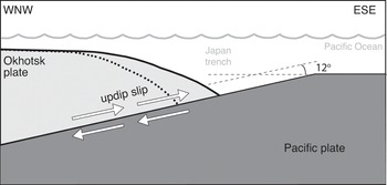
Figure 5.1 Cutaway view of Tohoku fault
Now it is fairly easy to visualize how large earthquakes occur on this fault. The Pacific plate is slowly getting pushed under the Okhotsk plate, but there are places where the two sides are locked together. The strain accumulates until it is enough to overcome the friction, and the two surfaces at the fault suddenly unlock. The upper surface jolts eastward and upward, releasing elastic energy in the form of seismic waves. The Tohoku earthquake ruptured an area of around 200 kilometres by 500 kilometres, and the entire rupture process took around 150 seconds. This motion also gave rise to a powerful tsunami that inundated the north-east coast of Japan. A detailed understanding of the rupture process, its connection to past and possible future earthquakes in the area, and the way in which it generated the tsunami, is of obvious importance for seismology, as well as the determination of seismic hazard along the coast of Japan.
The Tohoku earthquake was recorded on an unprecedented variety of instruments. Broadly, the data that were recorded for this earthquake can be categorized by the kind of phenomenon that was recorded. Seismic data are recordings of seismic waves. Strong motion seismic data is recorded at stations nearby an earthquake. These kind of data are recorded on several networks of different types of seismographs throughout Japan, including KiK-net, a network of over 600 strong-motion seismographs that are situated in boreholes; and K-NET, a network of over 1,000 strong-motion seismographs at the surface. Geodetic data are recordings of the deformation of the earth’s surface. Such data are typically recorded using GPS technology. Most of the geodetic data for the Tohoku earthquake was recorded on a network of over 1,200 GPS stations distributed throughout Japan, called GEONET. Tsunami data are recordings of the tsunami caused by the earthquake. This type of data was typically recorded by offshore wave and tide gauges. These three categories do not exhaust all the types of data that were recorded for this earthquake. In addition, there were important data recorded of the motion of the ocean bottom at seafloor geodetic sites, data from deep drilling into the fault zone after the earthquake and even gravimetric data recorded by satellites.
5.3 Rupture Narratives: From Data to Details
The data collected from the Tohoku earthquake are rich and diverse, but they consist of recordings of the downstream effects of the earthquake, such as ground motions that occurred far away from the fault. Such data do not immediately reveal any details about the rupture process. An initial step towards a reconstruction of the rupture process is the use of source models,Footnote 5 which, as we will see, take this downstream data and provide a detailed account – albeit an unreliable one – of the rupture process.
Most source models for the Tohoku earthquake have been constructed using a method called slip inversion.Footnote 6 A good example can be seen in Figure 5.2, taken from Reference Suzuki, Aoi, Sekiguchi and KunugiSuzuki et al. (2011). This is an early source model that was produced entirely from seismic data recorded at 36 stations located throughout northern Japan.Footnote 7 Let us first examine the large figure on the right. An outline of the northern part of the Japanese island of Honshu can be seen towards the left. Just off the coast is a rectangle, which has a length of 510 km and a width of 210 km, oriented at a small angle in the north–south direction. This rectangle is a representation of the fault. We are here viewing the fault from directly above (in contrast to Figure 5.1, which is a cutaway view). The dip of the fault cannot be seen in this view, but in this model the dip angle was set at 13 degrees to the horizontal.

Slip is a measure of how much the two sides of a fault moved relative to each other during an earthquake. The contours and shading on the figure to the right are an indication of how much various parts of the fault slipped over the course of the Tohoku earthquake. The darker the shading, the more slip occurred. According to this source model, there was an area of very large slip of around 48 m near the Japan Trench (towards the right edge of the fault). The series of 16 small figures on the left are miniature versions of the figure to the right. Each of these small figures represents the amount of slip on the fault in each ten-second slice of time from the beginning of the earthquake to the end (reading from top left to right, and then bottom left to right). As I described earlier, when an earthquake occurs, various parts of the fault rupture in succession. We can think of these as a series of snapshots of this rupture process as it propagates. If we allow for a wide definition of ‘narrative’ that includes visual objects such as diagrams,Footnote 8 we can view this series as a visual narrative of the rupture process, indicating spatial changes of the fault over time during the Tohoku earthquake.
Source model studies also provide more straightforward textual narratives of the rupture process, along with such diagrams. For example, Reference Suzuki, Aoi, Sekiguchi and KunugiSuzuki et al. (2011) provides the following:
The total moment rate indicates that first remarkable moment release started 20 s after the initial break, when the rupture occurred around the hypocenter. Then, at approximately 40 s, the rupture proceeded northward along the trench axis and towards the down‐dip direction. Somewhat later, the rupture also extends southward along the trench axis. The largest slip event occurred from 60 s to 100 s, with the rupture expanding towards the down‐dip direction from the area along the trench axis. In this stage, large slip occurred continuously far offshore of southern Iwate, Miyagi, and northern Fukushima prefectures. The last stage starts at around 100 s, where the rupture propagated southward in the area off Fukushima and Ibaraki prefectures. The entire rupture almost ceased within 150 s.
We can view slip inversion as taking seismic or other data as input, and outputting what I call rupture narratives, which are visual and textual narratives of a rupture process that includes quantitative details. Such details can include temporal details such as the timing of various sub-events within the rupture process. They can also include details about the rupture process as a whole, such as the total amount of slip that occurred at a particular part of the fault. Borrowing a term from Robert Meunier (Chapter 12), the rupture narratives produced by source models present themselves as ‘narratives of nature’ – narratives that recount a process as occurring in nature, independently of any human observers. As we will see, however, they are highly model-dependent – that is, many of the details within these narratives are artefacts of the data, techniques and assumptions that go into the source models.
An indication of this model-dependence is a wide variability among rupture narratives produced by source models of the Tohoku earthquake. Figure 5.3 is a comparison of 45 different source models of the Tohoku earthquake. Each of the lines represents the amount of total slip indicated by each source model. For ease of comparison, only the amount of slip along the corridor off the north-east coast of Japan indicated in the inset map is shown, extending from just underneath the coast to the Japan Trench. There is particularly wide variability in the up-dip regions, near the trench. Some models show slip of 50 m or more here, while other models indicate slip of 10 m or less.
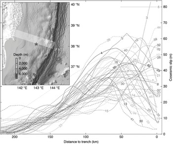
How could there be such discordance between rupture narratives produced by various source models of the same earthquake? Broadly, there are two reasons. The first has to do with differences in the type of input data. I have mentioned that the data that were recorded for the Tohoku earthquake can be categorized into seismic data, geodetic data and tsunami data. Source models have been constructed using all of these types of data. Different types of data are sensitive to different features of the rupture, and thus models that rely on different types of data tend to emphasize different features. The second reason has to do with differences in the methods used to construct source models. This can include differences in the parameterizations used, differences in the idealizations and assumptions that go into the models, and differences in the mathematical and computational techniques that are used.
5.4 Research Narratives: Distilling Details from Source Models
The first source models of the Tohoku earthquake were produced and published in 2011, within months after the earthquake. A large number of source models of the earthquake have been produced since then – by 2017 there were at least 45 of them (Reference Sun, Wang, Fujiwara, Kodaira and HeSun et al. 2017). From the start, there have been pronounced discordances between various source models of the earthquake. An important question for the reconstruction of the rupture process of the Tohoku earthquake has thus been: exactly what is one to conclude about the actual rupture process given the discordance between the source models? Is there a way of distilling out from these conflicting source models some set of rupture details that can be regarded as accurately representing the actual rupture process? One reasonable thought is that later source models are generally more accurate than earlier ones, since they presumably have more knowledge about the earthquake to draw upon. A more rigorous approach would examine in detail the evolution of source models since 2011 to determine whether indeed later models improve on earlier ones. This is the approach taken in Reference LayLay (2018), a review article of the Tohoku earthquake. Reference LayLay (2018) contains a very long and complex narrative that traces out the evolution of source models, with the aim of distilling out rupture details to which some degree of confidence can be attached. Borrowing again from Robert Meunier (Chapter 12), this is a research narrative – a narrative that provides an account of the activities of researchers.
Let us now take a closer look at the research narrative in Reference LayLay (2018). The general thrust of the narrative is to show how source models of the Tohoku earthquake have gone through an evolution, the result of which is that details in certain later source models have claim to being relatively accurate representations of details of the actual rupture process. For example, in a section of the narrative, Lay examines early source models based purely on geodetic observations made at onshore GPS sites. He notes that such source models ‘can provide good resolution of the spatial distribution of slip if the observation configuration is favorable’ (Reference LayLay 2018: 11). Unfortunately, it turns out that the observation configuration for the Tohoku earthquake is unfavourable – all of the GPS sites are on the Japanese mainland, which is on the down-dip side of the fault. This means that source models based purely on onshore geodetic data have poor sensitivity to slip that happens on the up-dip side of the fault, near the Japan Trench. This is significant, for, as Lay points out, although source models based purely on onshore geodetic data are largely consistent with each other, they are inconsistent with source models based purely on seismic data. Source models based purely on seismic data tend to show the largest slip happening up-dip, near the Japan Trench, as with the source model depicted in Figure 5.2, while source models based purely on onshore geodetic data tend to put the largest slip near the hypocentre, more towards the centre of the fault. One might surmise that the reason for this inconsistency is the unfavourable observation configuration for source models based on onshore geodetic data.
Recognizing this as a limitation, seismologists have attempted to address this problem in later source models utilizing onshore geodetic data by incorporating other types of data that are complementary to onshore geodetic data. Particularly important is a set of geodetic data taken by GPS/Acoustic stations located offshore, on the ocean bottom, which, according to Lay, has ‘proved transformative for geodetic models of the 2011 Tohoku earthquake slip distribution’ (Reference LayLay 2018: 12). Another important kind of additional data is time series data taken at GPS stations, called hr-GPS. Regarding the evolution of source models based on geodetic data, Lay states:
[T]here has been significant evolution of slip models inferred from geodesy, from the long smooth models with ~30 m peak slip near the hypocenter […] to much more spatially concentrated and up-dip slip models with peak slip of 50 to 60 m at shallow depth when using hr-GPS time series […] or from inclusion of up to 7 offshore GPS/Acoustic measurements in static inversions.
Significantly, these later source models are much more consistent with source models based on seismic data (note, for example, that the source model depicted in Figure 5.2 has a peak slip of 48 m in the up-dip, shallow part of the fault). In other words, the rupture narratives of these later source models look much more like the rupture narratives of source models based on seismic data.
Lay does similar analyses of the evolution of models based on other types of data, showing how later models have improved upon earlier models. Not only are the rupture narratives of later models more consistent with each other, but they are getting more detailed. He takes later source models that incorporate multiple types of data – called joint inversions – to be the most reliable. One reason is because data of different types can be complementary – they are sensitive to different aspects of the rupture process. Another reason is because the later source models generally address the shortcomings of earlier models. Lay summarizes the evolution of source models as follows:
The foregoing review of rupture models for the 2011 Tohoku earthquake shows progressive convergence of slip models, with slip being increasingly localized along strike and concentrated up-dip, extending all the way to the trench with slip ~50 m near 38.2°N. Over time the rupture models have progressed from quite smooth representations to more detailed slip distributions, especially for the geodetic and tsunami models. […] Some of the differences among current models may represent the different parameterizations, but the similarity of the majority of joint inversion models […] suggests that different parameterizations are at least not overwhelming the source information.
We can think of the research narrative provided by Lay about the evolution of source models as providing a justification that the details that appear in the rupture narratives of the later models are relatively accurate. Greater confidence is placed on the later joint inversion models, but no one model is taken to be best, and the amount of confidence one can place in a particular detail is ultimately based on a judgement that takes into account the commonalities between particular source models, limitations due to the datasets and methods of construction and the overall evolution of source models.
5.5 Integrating Narratives: Pursuing Further Evidence
Typically, in review articles, the details that are distilled from source models are strung together into a new rupture narrative that is independent of any particular model. This is a ‘narrative of nature’ – one that is taken to represent the best current estimate of the actual rupture process. There is such a narrative in Reference LayLay (2018), which he calls a ‘strawman reference model that distills the features that appear most stable and/or plausible’ (Reference LayLay 2018: 29). Although Lay calls it a model, it is not a model in the sense of the source models discussed earlier – it comes in the form of a textual narrative. As source models have evolved from the early source models based on single data sets to more detailed source models based on joint inversions, the details that were taken to be established about the Tohoku earthquake have also evolved. Thus, the model-independent rupture narratives that would be constructed by seismologists at any given time after the Tohoku earthquake would also evolve.Footnote 9 I will refer to rupture narratives of this type as integrating narratives because they are used as tools for integrating details of the rupture process with other seismological results.
In this section, I will show that integrating narratives play an important role in the production of new evidence about the rupture process of the Tohoku earthquake. First, let me provide, as an example, the ‘strawman reference model’Footnote 10 of Reference LayLay (2018):
In terms of the primary slip zone, the joint models including tsunami information […] provide good characterization of the rupture, with ~50 m of slip near or at the trench about 38° to 38.3°N. Shallow slip in the upper 10 km of the megathrust (from 8 to 15 km below the ocean floor) extends along strike from at least 37°N to 39.5°N, diminishing north and south of the central peak, which is near the site of the JFAST [Japan Trench Fast Drilling Project] drill hole. This is the Domain A zone of tsunami earthquake-like behavior discussed by [T. Lay, H. Kanamori, C. J. Ammon et al. ‘Depth-Varying Rupture Properties of Subduction Zone Megathrust Faults’, Journal of Geophysical Research 117(B04311): 1–21]. From 10 to 35 km depth, the large-slip region, with > 20 m of slip narrows to about ~150 km along strike, with the hypocenter within this zone, in what is called Domain B. Modest slip of 5 to 10 m is spread along strike, with down-dip Domain C concentrations of < 5 m offshore of Miyagi and offshore of Fukushima. These regions of prior M ~7.5 events during the past century appear to have re-ruptured with more high frequency radiation than the shallower regions.
This is just the beginning of the first paragraph of the narrative. The thing to note about this narrative is that it does not just string together well-established details from rupture narratives. It also makes reference to ‘domains’ of the rupture process, the ‘JFAST drill hole’, and past earthquakes.Footnote 11 The later parts of this narrative, not shown here, continue on to discuss studies of afterslip (ground motions that occurred after the earthquake), seafloor deformation observations and specific earthquakes of the past. Integrating narratives can also highlight loose ends and open questions. Let me note again that this integrating narrative is from a comparatively late stage of analysis of the Tohoku earthquake. Earlier integrating narratives tend to be less detailed, they draw fewer connections to other studies and their references to past earthquakes are framed in a more speculative mode.Footnote 12
Integrating narratives have provided a sort of frameworkFootnote 13 upon which certain questions about the Tohoku earthquake could be pursued. Some questions have to do with the connection between the rupture process of the Tohoku earthquake and its spatial and temporal context. More specifically, these questions can be about connections to past earthquakes, to seismic events immediately preceding the Tohoku earthquake, seismic events that came after it, and various features of the subduction zone on which it occurred, such as the locations of asperities, the distribution of accumulated strain, the composition of the rock in the subduction zone, and so on. Other questions have to do with anomalies or inconsistencies in the rupture process as laid out in the narrative. The pursuit of such questions has been a driving force for uncovering further evidence about the earthquake.
For example, a major open question has to do with the frequency characteristics of the rupture process. Just a few years before the Tohoku earthquake, a new technique for producing source models from seismic data, called back-projection, had been developed (Reference Kiser and IshiiKiser and Ishii 2017). Back-projection is sensitive to high-frequency seismic waves, and the source model it produces is a kinematic image, not of slip, but of seismic radiation energy release over time. Since most of the energy being radiated at any given time during an earthquake originates from the rupture front, the back-projection image can be taken to show a kinematic image of the rupture front during the earthquake. Early back-projection studies of the Tohoku earthquake were systematically discordant with early slip inversion studies. The back-projection studies indicated that most of the seismic radiation was concentrated in the down-dip part of the fault. On the other hand, slip inversion studies indicated that the maximum slip was in the up-dip part of the fault, and the area of very large slip possibly extended all the way to the trench (Reference Lay, Ammon, Kanamori, Xue and KimLay et al. 2011: 687). An early question about the rupture process was thus: why does back-projection appear to show that rupture occurred mainly down-dip, while slip inversion appears to show that the area of maximum slip was up-dip and close to the trench?
A possible answer is that different parts of the fault produced seismic radiation at different frequencies – the down-dip part producing more high-frequency radiation than the up-dip part. If this answer is right, then it gives rise to another question: is the difference in the frequency characteristics in different parts of the fault just a special feature of this particular earthquake, or is it a feature of the fault – in which case it ought to hold for other earthquakes as well? Reference Koper, Hutko, Lay, Ammon and KanamoriKoper et al. (2011: 602) suggested that the latter is the case – that the difference is due to depth-varying frictional properties of the fault.
The idea fits with the known history of the fault. The down-dip region corresponds to an area where large earthquakes of up to Mw 7.9 had repeatedly occurred over the past century, and these earthquakes would have had similar frequency characteristics as the down-dip part of the Tohoku earthquake. The up-dip region corresponds to an area that had not ruptured since 869 ce, but it also partially overlapped an area that is taken to have ruptured in 1896 during what is known as a ‘tsunami earthquake’. Tsunami earthquakes have characteristics like those exhibited by this part of the fault during the Tohoku earthquake – with large slip but slow rupture velocities, leading to relatively more seismic energy being radiated at lower frequencies.
In this view, then, each part of the fault has its own rupture characteristics that are constant across earthquakes (these are roughly the ‘domains’ that Lay refers to in the extract above). The unusual feature of the Tohoku earthquake was that it ruptured both regions at the same time, so it combined the characteristics of both types of earthquakes. Given this view, the next question to ask would then be why there are regions with different rupture characteristics within the fault – does it have to do, for example, with the composition of materials in different areas of the fault? This has been probed by the use of seismic wave tomography (Reference Tajima, Mori and KennettTajima, Mori and Kennett 2013: 27) and studies (such as JFAST) where holes are drilled directly into the sea floor in the fault area (Reference LayLay 2018: 28).
The pursuit of questions such as these has improved the picture of how the Tohoku earthquake fits into its spatial and temporal context – whether it is, in some sense, a repeat of particular earthquakes in the past, for example. It has also opened up new lines of research that have contributed new evidence about the Tohoku earthquake. In some cases, this new information has been utilized to improve source models – thus contributing to the evolution of source models, and indirectly to the evolution of the integrating narratives themselves. Thus, there is a sort of mutual evolution of source models and integrating narratives, resulting in a more highly resolved, and more ramified, picture of the rupture process of the Tohoku earthquake. That Lay refers to the most recent version of an integrating narrative as a ‘strawman reference model’ is an indication that this is very much an ongoing process.
5.6 Conclusion
In this chapter, I have examined the growth of knowledge about the rupture process of the Tohoku earthquake, with a focus on the role of narrative. I have described three kinds of narratives in this chapter: rupture narratives, research narratives and integrating narratives. I would like to end with some considerations about the functions of these narratives in contributing to the growth of knowledge about the Tohoku earthquake.
5.6.1 Narratives as Filters
Let me begin with rupture narratives. It is not entirely correct to say that source model narratives are the outputs of source models, for the direct outputs of source models are simply large sets of parameters. But these sets of parameters must be put into a cognitively useful form: the textual and visual narratives that I call source model narratives. These narratives are the result of filtering out some of the needless complexity in source models. They allow seismologists to focus in on significant details. They also allow seismologists to readily make comparisons between source models in order to look for commonalities and differences. Side-by-side comparisons of visual representations are particularly powerful – Reference LayLay (2018) contains page after page of diagrams where a half-dozen source models are compared side by side.
5.6.2 Narratives as Arguments
The research narrative provided a justification for distilling certain details from source models. Rupture narratives formed an important ingredient for the research narrative, because the latter required a comparison between source models, and analyses of the assumptions and methods that were used in their production. Another important element of the research narrative given in Reference LayLay (2018) was a story about the evolution of source models that attempted to make a case that later source models are more accurate. The research narrative pulled together and organized these elements into a prolonged argument that certain details in the source models can be pulled out and regarded as well established, independently of any particular source model.
5.6.3 Narratives as Unifying Instruments
Integrating narratives of the Tohoku earthquake have strung together well-established details that are distilled from source models, with the help of research narratives. They locate the rupture process within a spatial and temporal context, and they provide a framework for the pursuit of further questions that may open up new lines of research into the Tohoku earthquake and other past and future earthquakes. We might regard integrating narratives as instruments for unification – bridging various empirical avenues and strengthening connections between them, perhaps with the aim of achieving Whewellian consilience.
Thus, the three types of narratives I have considered, all, in different ways, have made contributions to the growth of knowledge about the Tohoku earthquake. The fact that several different kinds of narratives are utilized by seismologists is perhaps not that surprising. The work that narratives do in enabling the growth of knowledge in seismology and other physical sciences, however, still needs to be better understood.Footnote 14
6.1 Introduction
If you were thousands of years old, and in your youth had passed by the ancient city of Ur, Babylon,Footnote 1 at around 2000 bce, you might have been lucky enough to visit Simat-Enlil, King Shulgi’s daughter. Over a cold drink, she may have shown you a gift from her father: a bowl already over a hundred years old that he had inscribed as a gift to her (Reference ThomasonThomason 2005: 74). This is the first documented case of people reusing and reappropriating already old materials in historical archaeology. One and a half thousand years later,Footnote 2 Nebuchadnezzar and Nabonidus, successive kings of Babylon, excavated and restored earlier structures at Ur. While doing so, they re-incorporated into their architecture inscriptions made by different kings, thousands of years earlier. Due to written records, we also know that Nabonidus’s daughter, the princess En-nigaldi-Nanna, dug at the temple of Agade and had a room in her palace dedicated to items of antiquity, making her possibly the first known antiquarian (Reference DanielDaniel 1981: 14; Reference OatesOates 1979: 162). These instances of the curation of already old artefacts are usually understood by archaeologists to be efforts to reinforce authority through emphasizing a connection to past rulers or ancestors.
In prehistory (i.e., without the benefit of written information), our understandings are built through narrative explanations based on the suite of physical evidence we encounter. The amount and nature of this evidence vary wildly – sometimes preservation is excellent and at other times very poor – but in general terms there is more evidence from time periods closer to the present day than from the more distant past. Already old materials incorporated into later deposits have been noted by archaeologists at prehistoric sites (Teather 2018; Reference Knight, Boughton and WilkinsonKnight, Boughton and Wilkinson 2019), and recent applications of absolute dating methods in prehistory have led to more instances of out-of-time artefacts being uncovered. I will argue in this chapter that this greater focus on attempting to ascribe more precision to an archaeological event has forced archaeologists to confront their own assumptions of what kinds of time they are trying to measure, and use, to frame accounts of past lives.
Archaeological information can be an important source of identity for human societies, providing an alternative narrative of life in the past and its connection to the present that can sit alongside origin myths, religion and history. As a uniquely integrated discipline of history and science, archaeology has made increasingly sophisticated use of narrative tools in the last 30 years. While it has always used narration to report and discuss evidence retrieved from past people’s lives, this has been problematic. Narrative approaches have sometimes been seen as unduly historical and not scientific or objective enough; but scientific results are equally understood to be subjective and selective (or, at least, ‘theory laden’) and require explanation. In undertaking archaeological analysis, we are inextricably tied to both disciplinary approaches. This chapter traces the structure of knowledge creation in archaeology, how this applies to measuring time and how these are brought into coherent narrative form by archaeologists. In conclusion, archaeological information both contains stories and suggests stories: some that are ours and some that belong to the past.
6.2 Archaeological Knowledge and Narrative
6.2.1 What Is an Archaeological Narrative?
The craft of building an archaeological narrative is referenced in the profession as a type of interpretation, and in archaeology the study of types of interpretation, while often epistemological, is referred to as ‘archaeological theory’. Archaeological interpretation is therefore the creation of narratives about the past, based on the evaluation of different kinds of facts.Footnote 3 For archaeologists, facts encompass a wide range of different categories of evidence. These might be historic, artefactual or architectural; comprise chemical or biological information; and, for both sets of these types of facts, be comparative or analogous. Reference Wylie, Howlett and MorganWylie (2011: 302) has referred to these as facts of the record/mediating facts; and historical facts, which themselves comprise two types of facts – facts of the past and narrative facts. It is useful for the purposes of this chapter to think of facts as defined by Reference Haycock, Howlett and MorganHaycock (2011: 424): ‘a fact is not of necessity something that is true; it is rather something that is taken to be true on the basis of current evidence in the context of a particular scaffolding of knowledge, ideas and beliefs that supports it’.Footnote 4
Archaeology has different, and separate, types of scaffoldingFootnote 5 that each constitute a body of interrelated facts, that themselves are composed of combinations of knowledge, ideas and beliefs of different kinds. For half a century, archaeologists have been familiar with visualizing this process, with much less sophistication than Reference Chapman and WylieChapman and Wylie’s (2016) work, as a ladder of inferenceFootnote 6 where the further one travels up the ladder of knowledge, the further one is removed from the archaeological facts (or facts of the record, as Reference Wylie, Howlett and MorganWylie (2011) might say). If we continue for the moment with a ladder analogy for scaffolding in archaeology, we can begin to see the types of scaffolding as separate self-supporting pillars of knowledge, or chronicles, that create genealogiesFootnote 7 by a process of colligation (Reference MorganMorgan 2017: 88–89).Footnote 8 For this chapter it might be easier to visualize them as subject-based – for example, one genealogy might be that of pottery production (following a particular technical and historical trajectory and incorporating chronicles encompassing the types of clay, temper and firing times, experimental work and ethnographic analogy); another genealogy might be an account of animal husbandry (following animal domestication, genetics, behaviour, meat or dairy yield and comparative ethnographic information of the composition of different kinds of herds for different economic purposes). For example, in northern Europe the remains of sheep, cattle and pig in domestic species form a consistent contribution to past economies from 4000 bce to the modern period, but their proportion in deposits changes depending on the subsistence focus.Footnote 9 The chronicles might be broadly the same in many instances, but branch into different genealogies and narratives.
6.2.2 Construction of Archaeological Narratives
Narratives in archaeology weave between these chronicles and genealogies, as if with ribbon, creating individual cat’s cradles by encompassing different facts from different chronicles and genealogies. For example, I conducted a synthesis of prehistoric human burials with strike-a-light kitsFootnote 10 that determined that the overwhelming majority occurred with male burials between 2200 and 2000 bce (Reference Teather and ChamberlainTeather and Chamberlain 2016). While already considered to be a gendered practice, this research showed it was more common, very strongly male-related, often seen in higher status burials and, as a product of new radiocarbon dating, the duration and peak occurrence of the practice could be ascertained. In terms of scaffolding, this paper relied on many different chronicles of knowledge: experimental work; chemical work on the degradation of iron pyrites in soils over time; a genealogy of situating the practice within European prehistoric analyses of similar types of burials; and finally, the metaphorical work of Reference Lakoff and TurnerLakoff and Turner (1989) (a genealogy based on the use of textual analysis and material culture in archaeology) to suggest that death may have been seen as a type of journey for the dead men during this time period and requiring a portable source of light and/or heat. Each of these elements as brought to that paper have their own histories and scaffolds of knowledge in archaeology and cognate disciplines of anthropology and ethnology, but it was the authors’ preference and choice to bring them together in this particular narrative. Other authors could use the same starting point of evidence and produce a different cat’s cradle of narrative.Footnote 11 The success of this particular approach was that it has stimulated more attention during excavation to record and identify these otherwise quite functional and unremarkable objects; the thorough synthesis accompanied with a compelling narrative proposing a rich metaphorical significance has affected field practices. In Berry’s terms (Chapter 16), the authors are present in the archaeological narrative through this process. Yet, the motive of the original research question or puzzle that stimulated that work is not actually mentioned in that paper.Footnote 12 As a specialist in artefacts made from chalk in the Neolithic, I have proposed that most chalk artefacts mimic artefacts made from different substances, such as stone or wood (Reference Teather and ShaffreyTeather 2017; Reference Teather, Chamberlain and Parker PearsonTeather, Chamberlain and Parker Pearson 2019). I was puzzledFootnote 13 by chalk ‘charms’Footnote 14 found in a small number of burials of predominantly women and children, and their visual resemblance to iron pyrite strike-stones that were in a few adult male burials (Figure 6.1).
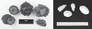
Figure 6.1 Iron pyrites (left) and chalk charms (right) from the burial of a female, dated to 3600 BCE
No recent research had been conducted on strike-a-light burials so I had to complete it myself and having done so can argue (and will do so further in a monograph in preparation) that strike-a-light burials may have been male-dominated in this period, but that there was a metaphorical past connection in a different material within the burials of women and children. Therefore, the strike-a-light burials are male-gendered, but a similar practice included women and children in a different, and potentially socially subversive, way. In order to argue that position and create a convincing narrative, the research had to be completed in this sequence.
These examples show that archaeological narratives appear to map well onto a narrative science framework. I will now turn to focus on archaeological dating methods and how these fit into this proposal.
6.3 Archaeological Dating
Chronologies in archaeology are manifold and can refer to temporal changes in certain types of artefact or in modes of an economy or social system. In effect, they are types of chronicle that seek to order selected events by the inclusion and exclusion of information. Relative and absolute chronologies (Figure 6.2) sit side by side in archaeology and can include many different facts of the record, but are constructed in different ways.

6.3.1 Relative Dating
In the history of archaeology, an interest in relative chronology began in earnest with typological studies of antiquities that initially made a categorical separation of geological objects and human-made artefacts. In the 1880s, Oscar Montelius created extensive relative typologies of archaeological artefacts across Europe with the goal being to devise a chronology for the broad cultural sequence (see Reference TriggerTrigger 1989: 155–156). Yet it was Christian Jürgensen Thomsen who advocated an approach to determining chronology through the typology of ‘closed finds’, representing objects found together in burial, hoard or other groupings, which suggested they were deposited at the same time (Reference TriggerTrigger 1989: 76). As a result, he was able to organize prehistoric material culture into a Three Age System that defined a narrative progression from the Stone Age to the Bronze Age and the Iron Age (Reference MarilaMarila 2019: 94–95). The left-hand side of Figure 6.2 shows the end phases of the Stone Age into the Bronze Age.
Therefore, it was not only the individual artefact that was important but what it was found with – i.e., its systematic co-occurrence with other artefacts. For example, it was not simply that a bronze axe was discovered with a particularly distinctive pottery vessel together with a human burial in a mound, but rather that bronze axes were repeatedly found with that type of pottery with burials in those types of earthen mound. Thus, the first chronologies in archaeology were the product of a scaffolding of facts – such as the typologies of artefacts commonly found together and through stratigraphic sequences,Footnote 15 where deposits are discovered above or below other deposits. The terminologies for this are specified as the terminus post quem and the terminus ante quem: something has to be later (post) or earlier (ante) than something else either because of where it appears in the archaeological sequence or what it contains, but a firmer date cannot be specified. For example, a coin hoard might contain currency minted in ad 83, ad 104 and ad 200, and therefore it would have a terminus post of ad 200 in that it would have had to have been deposited after ad 200, even though it contained earlier coins. If this hoard were buried under a sixth-century Anglo-Saxon brooch, the coin hoard would have been deposited between ad 200 and 600, as the brooch provides a terminus ante of ad 599.
Relative dating in archaeology is therefore predicated on two distinctions: first, that combinations of portable material culture,Footnote 16 as assemblages,Footnote 17 are distinctive to a particular culture and indicative of the subsistence, economics and social relations of that past population; and second, that each archaeological context such as a burial is physically separated from another context as a time capsule (making it a closed context) that we can discern through stratigraphic excavation. Therefore, typologies (systems of classification of evidence into distinct categories) and seriation (the sorting of evidence into a temporal sequence) were first established alongside chronology and relative dating, and all continue to be core elements of archaeological research practice. Assemblages, formed of typologies, closed contexts and seriation, can be seen as the scaffolding for chronicles, that form the basis of narratives.
Types of comparative assessments are also key to relative dating but might be seen more effectively as genealogies rather than as chronicles (Berry, Chapter 16). For example, aerial surveys using light detection and radar (LiDAR), or other remote sensing methods, produce images that can be compared with known excavated sites to produce an initial identification and assessment. The kinds of question that are approached here primarily rely on size and form: a 30 m circular banked and ditched enclosure may suggest an earthen henge monument like Avebury in Wiltshire (refer to the left-hand side of Figure 6.2), whereas a 10 m × 10 m square enclosure suggestive of stone-built foundations may indicate a Romano-Celtic temple.
Broader-scale narrative sequences are therefore built from aggregations of evidence from many excavated sites. Alongside typological considerations of materials present in archaeological deposits, they enable temporal chronologies to be brought together. Only limited comparisons may be possible between different archaeological sites unless cultural expressions such as pottery, buildings or monument styles are widespread and very similar. Where these are present, it allows for broad regional- and continental-scale syntheses, a particular kind of narrative. Relational dating is therefore reliant on a series of comparative interpretations of artefact and site typological data that are assessed and applied to each example, and are effectively genealogies. These are nested within a wider geographical and temporal understanding of comparative data as chronicles. Narratives can emerge at these different scales: the artefact, the period, the site, the region, the continent. While relative chronologies still have their uses for broadly determining an outline chronology, they can fail where we cannot easily determine chronologies from artefacts (e.g., through typologies where artefacts are degraded/when material culture changes little through time) or when we attempt to compare sites that are geographically separated.
6.3.2 Absolute Dating
The advent of absolute scientific dating in the mid-twentieth century had a significant effect on archaeological chronologies. It meant that materials and deposits could be placed within a chronicle of a measured time-scale of calendar years (refer to the right-hand side of Figure 6.2) rather than being reliant on relative factors alone. Initial methods included dendrochronology (tree-ring dating) and radiometric (commonly, radiocarbon) dating. Radiocarbon dating measures the decay of an unstable isotope of carbon from the time the living organism ceased respiration, and as such provides a date of ‘death’ as a probabilistic range.Footnote 18 Dendrochronology can identify the year at which the living tree was felled, and as such is potentially much more accurate than any other form of dating but is only applicable to suitable surviving timbers that preserve a sufficient number of tree rings to allow them to be matched to a reference chronology. Direct dating methods such as these are preferred particularly for human and animal remains, and due to the prevalence of these organic materials in deposits, radiocarbon dating has proved to be a key tool in discerning chronologies.
However, these have now been joined by further physico-chemical dating methods. These include uranium series dating of cave minerals, optically stimulated luminescence (OSL) to date sediments to when they were last exposed to sunlight, and palaeomagnetic dating that can be used to date deposits such as hearths that have been subject to an episode of burning. Amino acid racemization measures time-dependent changes in protein molecules (Reference Demarchi, Collins, Rink and ThompsonDemarchi and Collins 2014) and ceramic rehydroxylation (RHX) is able directly to date pottery through the chemical reaction on firing the pottery.
Indirect methods are also increasingly important. For example, molecular clock (or coalescent analysis dating) analyses molecular diversity to determine the sequence and timing of past demographic and evolutionary events that have left traces in both modern and ancient genomes. This means that we can assess the diversity of ancient populations in particular areas, and pinpoint times that they began to diverge from each other. These different methods speak to the different aspects and scales of the archaeological record; whether the research aim concerns the activities of living people such as firing pottery, or a much wider scale such as questions of genetics and evolution. They all result in establishing archaeological chronologies for the methods and assist in creating genealogies and narratives that refine archaeological sequences and constrain the duration of temporal events.
Absolute dating is seen as a preferred and more robust, scientific way of determining ageFootnote 19 as it can order events and material culture within a fixed temporal chronology and make it possible to compare within and between sites in a greater range of archaeological settings. While it might be considered better and more objective science to discard the application of anything but the broadest use of relative chronology, there are some instances where relative dating techniques are the preferred method. Relative chronologies are still very informative for styles of prehistoric rock art, which by their nature are often impossible to date using absolute methods. For historic periods, relative chronologies such as seriation are more often employed as many of the dating methods (apart from dendrochronology) are not more accurate. Therefore, clay pipes, for example, can be attributed to periods of manufacture and sometimes individual makers (e.g., Reference WilliamsonWilliamson 2006), and as they are commonly discarded when broken their period of use is reflected in deposits.
In summary, our archaeological chronologies have been subject to a shift and expansion in reasoning with the advent of the direct dating of materials. From a relative-based chronological approach, which is inherently genealogical, we now include an absolute chronology, or a chronicle, that does not rely on the storied or narrative aspect of the archaeological record but simply ranks the dates in sequential order (Figure 6.2, right-hand side). Absolute dating chronicles can be used to generate different genealogies and narratives without attention to the existing genealogy of relative chronology. This has resulted in a suite of new approaches to examining archaeological time.
6.4 From Dates to Narratives: Impacts of Recent Studies
As detailed above, relative and absolute dating provide different ways to build narratives. For relative chronology, narratives are built piecemeal from the contributions of seriation, typologies and closed contexts – often by individual scholars working on sets of material with continual reference to the existing genealogies and chronicles. When syntheses are produced, they are agreed in chronicles by the process of accepting individual facts within the scaffolding of each chronicle. Therefore, these have been subjected to continuous revision and refinement over time (Reference Chapman and WylieChapman and Wylie 2016), as new discoveries have been made or inferences or assumptions have been successfully challenged. This process produces rich and subtle narratives that often incorporate previously overlooked evidence and challenge earlier interpretations or narratives, such as the Glastonbury Iron Age village where the excavators’ results were revisited and reworked five times between the 1960s and 1990s (Reference Chapman and WylieChapman and Wylie 2016: 108–136).
On a wider scale and using data from the British and European Neolithic period, the span of data derived from relative dating originates from the accretion and consensus of primary analyses of archaeological finds. These initially consist of collections of multi-authored specialist reports of pottery, flint and other materials, that when taken together lead to a consensus of date or date range that subsequently fits into the broader relational chronological framework. At this stage, it is usual for a few ‘range-finder’ radiocarbon dates to be obtained to confirm the proposed artefact-based chronology. Therefore, at an initial and primary assessment stage, three to five radiocarbon dates may be taken per site to confirm and establish, or conversely challenge, the range of activity and sequence proposed through the relative dating methods. When information from many sites is aggregated, this results in a fairly even spread of absolute dates throughout the chronological sequence, as seen with the numbered dates on the right-hand side of Figure 6.2.
In the last decade and a half, advanced computational approaches have permitted new analyses of absolute dating evidence undertaken on archives of previously excavated materials that have challenged this traditional means of narrative building in archaeology. Intensive radiometric dating studies on archival material that have often focused on a particular category of site or research question have increasingly been undertaken. These dates supplement the range-finder dates typically gained through excavation and have the effect of creating blocks of data in the temporal framework and consequently an uneven distribution of information (please refer to the tightly spaced lines on the right-hand side of Figure 6.2). Two approaches have been particularly prominent: new absolute dating on sequential stratigraphic layers within archaeological deposits to produce Bayesian statistical analyses of site chronologies; and large-scale geo-spatial analysis of aggregated radiocarbon dates. These projects produce narratives and chronologies that are based on either inclusive or reductive reasoning. Inclusive narratives use absolute dating to establish how events are chronologically and spatially related. They are inclusive, as they seek to address all the findings uncovered, and they are narrative in that they provide an explanation for those findings through attention to the type of artefactual material under study and the sequence revealed. Reductive chronologies use absolute dating to provide a more precise date for an event. They are chronologies in that precise time measurement is their goal; and they are reductive in that they exclude dating evidence that does not easily confirm their chronological goal. This is because they assess any type of material culture as solely contributing in terms of chronological (and not cultural) evidence.
6.4.1 Case Studies Producing Inclusive Narratives
Absolute dating can help archaeologists establish how events are chronologically and spatially related. When projects consider all dates obtained and attempt to explain them by attending to questions of artefact type and sequencing, they produce inclusive narratives. Two examples of inclusive research-led projects that involved gaining new radiocarbon dates follow.
Reference Parker Pearson, Sheridan, Jay and ChamberlainParker Pearson et al. (2019) presented the results of a large-scale project on dating the Early Bronze Age phenomenon of Beaker burialsFootnote 20 in Britain that date from 2600 to 1700 bce. The aimFootnote 21 of this project was to discover and assess the level of mobility of those buried people during their lives. The skeletal remains from 370 individuals were investigated, with 17 found to date earlier than the period under study and 19 later, together with a number of examples that could not be dated by absolute methods (Reference Parker Pearson, Sheridan, Jay and ChamberlainParker Pearson et al. 2019: 426). Constraining the dates of the ‘Beaker phenomenon’ is an important archaeological question but one that has become more current due to ancient DNA analyses that have suggested that Beaker people arrived in the UK as migrants from continental Europe (Reference Olalde, Brace, Allentoft and ArmitOlade et al. 2018).
The second project directly dated archival material from mining and quarrying sites that were thought to date from the start of the Neolithic in Britain and continental north-west Europe (6500–1500 cal bc: Reference Schauer, Shennan, Bevan and CookSchauer et al. 2019b; Reference Schauer, Bevan, Shennan and Edinborough2019a; Reference Edinborough, Shennan, Teather and BaczkowskiEdinborough et al. 2020). The goal here was to determine if stone axes (the primary products of mines and quarries) were in increased demand for clearing forest during the economic change to agriculture at this time, and, if so, precisely when this occurred.Footnote 22
For both projects, the radiocarbon dates as new ‘facts of the record’ are treated as fully correct, even if they do not answer the research question. The impact of the small proportion of dates that fall outside the timespan of the research question is minimal, but the anomalous dates are nonetheless recorded and discussed informatively. In the first example on Beaker burials, the absolute dating related to one phenomenon (the death and subsequent burial), the one dating material type (the body) and the accompanying analyses on mobility (the body) have created a different genealogy of Beaker practices through new radiocarbon dates. Each burial is contextualized in the project publication within its geographical location at death, location/s of the life of the past person, the character of the grave (mound/cist/cut grave) and its accompanying grave goods. In terms of evidence, it could be argued that this research dating programme has enriched the primary archive and allows further reconsideration of that primary archive in future through informing different chronicles, even when the information is unexpected. The second example of the summed probability dating has enhanced the suite of absolute dates available for mining and quarrying and so enhanced the primary archive. In both cases, the computer modelling for activity trends takes place with the achieved raw dates to detach them from their immediate context within the archaeological siteFootnote 23 and to re-contextualize the dates as proxies for population.Footnote 24
At these different scales of analysis, the recontextualized narrative permits the puzzle to be convincingly answered while the non-compliant results are explicable either by producing new knowledge, or by reassessing the facts of the record. For flint mining, radiocarbon dates from Church Hill, West Sussex, demonstrated that there was an early Bronze Age phase that had been previously suspected but not substantiated (Reference Edinborough, Shennan, Teather and BaczkowskiEdinborough et al. 2020). In the case of Beaker human remains from Linch Hill, Oxfordshire, that surprisingly produced a Neolithic radiocarbon date, it was suggested that the human remains from this site were mislabelled at some point post-excavation. These remains now have the correct attribution for future researchers (Reference Parker Pearson, Sheridan, Jay and ChamberlainParker Pearson et al. 2019: 426); the known fact has been corrected. Therefore, inclusive narratives seek to use the chronicles created to produce as many genealogies and narratives as are required, even if they were not the primary goal.
6.4.2 Case Studies Producing Reductive Chronologies
Some projects use absolute dating with the unique aim of precise time measurement. In the process, they evaluate material culture only in chronological (not cultural) terms, while excluding dating evidence that doesn’t ‘fit’ their chronological goal. Such studies tend to produce reductive chronologies.
Bayesian analysis has been an innovation in archaeology in recent years that uses a statistical process to constrain the probability range that radiocarbon dates provide, thereby increasing dating precision. This type of methodology is increasingly used on large datasets to examine trends,Footnote 25 but is also used by some researchers for analyses within a small physical scale of archaeological remains in a stratigraphy-based Bayesian analysis. Here, the stratigraphic record is used to enable the research team to restrict the radiocarbon dates by considering whether a datable deposit is higher or lower in the depositional sequence than another datable deposit (terminus post quem or terminus ante quem).
‘Gathering Time’, a project led by Alasdair Whittle early this century, focused on dating causewayed enclosures, an early Neolithic type of monument.Footnote 26 Deposits from ditches were multiple dated to ascertain an accurate construction date in order to map the temporal distribution of UK enclosures. For example, at Whitehawk enclosure, in Sussex, an additional 38 radiocarbon dates were gained from deposits in the 4 concentric ditches in addition to the two dates already obtained from Ditches III and IV (Reference Whittle, Healy and BaylissWhittle, Healy and Bayliss 2011: 214–226). The original two post-excavation radiocarbon dates suggested that the enclosure was built and used within a broad range of time between 3710 and 3090 cal bc.Footnote 27 New dates were taken assuming that the digging of the original ditches and the accumulation of chalk rubble within them constituted one phase and that silting above this was a secondary phase. Using their analyses,Footnote 28 the conclusion is that Whitehawk was constructed between the mid-37th and 36th centuries bc, and ‘in primary use for 70–260 years (95% probability), probably for 100–115 years (4% probability), or 155–230 years (64% probability)’ (Reference Whittle, Healy and BaylissWhittle, Healy and Bayliss 2011: 226). This project concluded with assessing the radiocarbon dates from enclosures, alongside other modelled regional dates, to propose that, as a phenomenon, causewayed enclosures were constructed at slightly different times in different regions in southern Britain, although all between 3710 cal bc and 3630 cal bc, with some later in Wales (to 3550 cal bc: Reference Whittle, Healy and BaylissWhittle, Healy and Bayliss 2011: 694). Apart from these new chronicles, the further narrative conclusions of this project are based on the estimation that the Neolithic transitionFootnote 29 began in each of the causewayed enclosure areas two hundred years prior to the actual construction of causewayed enclosures, thus the chronicles have been combined with other models in order to create a plausible narrative for the Neolithic transition (q.v. Reference Whittle, Healy and BaylissWhittle, Healy and Bayliss 2011: 727–729).
In order to be successful, this method either completely excludes – or assigns very low prior probability weightings – to radiocarbon dates that are regarded as erroneous or that simply lie too far outside the acceptable range of possible dates. This rationale creates new chronicles by detachment, permitting the separation of dates into acceptable and unacceptable categories that lead to inclusion or rejection. The expectation is for conformity. By filtering the dates, two chronicles are created: one normative and used as a source model and one that remains peripheral.Footnote 30 The new normative chronicle is based on this filtered data, and these chronicles are aggregated to include multiple archaeological sites that have been assessed in a similar way (another chronicle) to lead to an overarching narrative of the beginning and end dates of particular types of site. A genealogy is not necessarily produced (as chronology is the goal, not the identification of causation), but rather new chronicles for each archaeological site – that are then aggregated again into another larger chronicle. The narrative is created through reference to existing archaeological genealogies.
These stratigraphy-based Bayesian methods have been responsible for a greater number of radiocarbon dates as facts, but the density of the information is intra-site rather than inter-site. The multiple radiocarbon dates produced are separated in the archaeological record not by archaeological site but by archaeological layer.Footnote 31 They are therefore not representative of different activities in different places, but rather episodes of similar activity at the same location in a broadly temporally similar or adjacent time.
6.4.3 Summary: From Dates to Narratives
The absolute dating of archaeological material as a separate and secondary procedure that takes place on already excavated material held in museum archives is often completed with a particular research question in mind. From this initial stage, a new chronicle begins to be constructed that will ultimately assess certain categories of archaeological material, and not others. Monuments or burials that were excavated by different people, decades apart, become one synthesized category for the purposes of the project, producing new chronicles. These may lead to new genealogies and narratives at different scales, although that is not always certain. If the research question is primarily temporal, the narrative implications may be largely to construct new chronicles. Whatever their primary aim may have been, their enduring influence is in enhancing the archaeological record with more absolute chronological data as facts of the record.
Alongside these new methods, new ways of accessing radiocarbon dates have also been developed. For example, the University of Kiel in Germany has created RADON,Footnote 32 a free online database of radiocarbon dates across Europe. It is possible to compare the radiocarbon dates gained on archaeological material from different countries and their regions through this database. Interestingly, the UK has almost double the number of radiocarbon records of any other country,Footnote 33 perhaps reflecting an uneven approach to dating in the UK – or perhaps the inclusion of UK dates in the database has been higher for other reasons. Nevertheless, in the RADON chronicle of chronology, any dates from peripheral chronicles and excluded from a stratigraphically based Bayesian narrative have been reapplied to their site context: the distinction in the Bayesian narrative between ‘right’ and ‘wrong’ dates is removed. This reincorporation is important, as it allows all the primary data for each site to be held together as a single site chronicle.
6.5 Conclusion
This chapter began with a discussion of the use of already old material culture in later deposits in ancient Babylon. Between the third and first millenniums bce, the connection between the curation, deposition in graves and/or powerful display of material culture initially had the purpose of legitimizing the power of individuals in their leading societal role, both locally and regionally. In the British Neolithic (4000–2000 bce), it is possible that old bones were already incorporated into pits or burial chambers, which may have been for the purpose of integrating past material with those of that present (Teather 2018), and, later in prehistory, human bodies appear to have been deliberately mummified, curated and buried at a later date (Reference Booth, Chamberlain and Parker PearsonBooth, Chamberlain and Parker Pearson 2015). For archaeologists, time and temporality are different faces of the same coin: time is simply a clock; temporality encompasses the human experience of time and is not easily measured.
I have sought to discuss how narratives in archaeology are created through chronicles and genealogies. Archaeologists are familiar with only achieving a temporary success with our narratives; research in our archives and in the field is a continual process, and new discoveries can quickly destabilize existing narratives. By separating our narratives into the use of facts, chronicles and genealogies, it allows us to comprehend the complex structure of archaeological knowledge and how we construct it. New information is readily incorporated into our existing genealogies and chronicles.
I have chosen to discuss chronology in archaeology, and how absolute dating methods have moved our primarily genealogical reasoning into establishing chronologies which, in the end, produce only chronicles. Further, the different methodologies within absolute dating projects have resulted in a diversity of composed narratives. In particular, the creation (or not) of filtered chronicles and use of detached narratives (narratives detached from context) have been seen to be pivotal to this process, and I have termed these inclusive narratives and reductive chronologies.
While more absolute dating allows us to create more chronicles of absolute chronologies, these are not equal. Some will provide us with more adjacent temporal moments that do not necessarily produce better understandings of the archaeology but answer questions of time. Normative approaches will produce a normative view of human behaviour. But the peripheral, inconvenient and subversive facts construct entirely different chronicles, genealogies and narratives. These are where the human stories lie.Footnote 34


 Open access