- The time registered on the airplane clock is both a coordinate time and a proper time. It is the proper time of the airplane: that is, if that time says thirty seconds have elapsed, then exactly thirty seconds have elapsed for anyone on the airplane. It is also the coordinate time in the reference frame of the airplane. (Note that the airplane—unlike, say, Emma the twin—remains in one inertial reference frame throughout its journey.)
- The time registered on the mountain clocks is a coordinate time but it is not a proper time. It is the time between these two events in the inertial reference frame of the mountains. But there is no object in that reference frame that experiences both of those events, so it is not a proper time.
The airplane plays a very special role in this scenario, by representing the reference frame in which both events happen at the same place. This means, among other things, that…
- The airplane’s reference frame is the only frame that can measure both a coordinate and a proper time between these two events.
- Any other coordinate time will be longer than the airplane’s; any other proper time will be shorter than the airplane’s. All of this follows from the dictum that “moving clocks run slow.”
- The time the airplane measures is also the spacetime interval between the two events (a topic we will introduce a few sections hence), if you use relativistic units
 .
.
Asher plays the same role in the twin paradox, since the two events (Emma’s departure and her arrival) occur at the same place in his reference frame.
We know that at the beginning of the journey, as the airplane passed Mountain A, the clock on Mountain A read ![]() . And we know that—in the airplane frame—the mountain clocks advanced 1/4 of a second during the journey. So at the end of the journey, the Mountain A clock must have read
. And we know that—in the airplane frame—the mountain clocks advanced 1/4 of a second during the journey. So at the end of the journey, the Mountain A clock must have read ![]() .
.
To put it another way:
- The event “Mountain A clock reaches
 and the event “airplane reaches Mountain B” are simultaneous in the airplane frame, but not in the mountain frame.
 - The event “Mountain A clock reaches
 and the event “airplane reaches Mountain B” are simultaneous in the mountain frame, but not in the airplane frame.
- Because the junction is moving at speed
 , it has moved a distance
  .
. - So at
 it was at position
  .
. - At time 0 the number of red rulers between the origin and that junction was just the position . But the blue rulers are shortened by a factor of
 . So the number of blue rulers between the origin and that junction was
  .
.
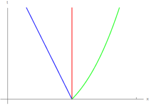
The world lines of an object at rest (red), an object moving at a constant negative velocity (blue), and an object with a positive velocity, slowing down (green).
It’s not obvious what happens to that formula as ![]() , is it? But it’s much clearer to look at it the other way; you can readily see that as
, is it? But it’s much clearer to look at it the other way; you can readily see that as ![]() , that makes
, that makes ![]() .
.
So as you add more and more energy—that is, you keep exerting force to accelerate an object—its speed does not approach infinity as it would in classical dynamics. Rather, its speed asymptotically approaches ![]() .
.
We see this in particle accelerators in real life, where adding more and more kinetic energy accelerates particles to very high percentages of the speed of light, but never past.
- The horizontal component of the vector tells us the distance traveled.
- The vertical component tells us the time elapsed, multiplied by
 .In relativistic units
  so this is numerically equivalent to the time elapsed in whatever units you are measuring. For example, if the vertical component of
  is 4 light-years, then the journey took four years.
 - The direction of that vector relates to the speed of the journey. As we have discussed before, speed=1/slope, ranging from a vertical line (speed=0) to a
 line (light). No journey could have a slope below that
Note that all of these components are measured in your coordinate frame (presumably the one in which you drew the ![]() and
and ![]() axes). Observers in different reference frames would measure different components for
axes). Observers in different reference frames would measure different components for ![]() because they would measure different distances and times for the journey.
because they would measure different distances and times for the journey.
1. Run the double-slit experiment one photon at a time, but put detectors at both slits so you can measure a photon going through the left slit, the right slit, or both simultaneously.
Write down your answer. Then click here to see the experimental result.
2. The same as above, but with no detector in the right slit. (If the detector goes off, a photon went through the left slit. If something appears on Wall B but the detector didn’t go off, the photon passed through the right slit.)
Write down your answer. Then click here to see the experimental result.
3. Repeat the original experiment (no detectors) but emit electrons—still one at a time—instead of light.
Write down your answer. Then click here to see the experimental result.
1. Plugging in ![]() turns this equation into
turns this equation into ![]() . At that instant the string looks like a sine wave with amplitude
. At that instant the string looks like a sine wave with amplitude ![]() and wavelength
and wavelength ![]() . (At other times the wave has different amplitudes, but always the same wavelength.)
. (At other times the wave has different amplitudes, but always the same wavelength.)
2. Plugging in ![]() turns this equation into
turns this equation into  . That particular point on the string is oscillating with amplitude is
 ![]() and period
and period ![]() . (At other locations the wave has different amplitudes, but always the same period.)
. (At other locations the wave has different amplitudes, but always the same period.)
- Because systems tend to accelerate toward regions of low potential energy, the object begins by moving to the right. It picks up speed as it moves: that is, it converts potential energy to kinetic energy.
- At
 the object reaches its minimum potential energy and its maximum speed.
 - To the right of the object is still moving to the right (because of the built-up inertia) but the force is now pushing it to the left, causing it to slow down.
- The object comes momentarily to rest at
 , at a spot where
  is exactly as high as it was at
  . That is to say, the kinetic energy has now been converted back to potential energy.
 - Then the object begins to move leftward again. It will rock back and forth between and
A classical particle in an infinite square well would bounce back and forth between the edges of the well. Assuming no energy is lost, it would keep doing this (at constant speed) forever.
- Continuity at :

- Continuity at
 :
: 
Differentiability requires that their first derivatives also match. Differentiating the solutions and then plugging in ![]() and
and ![]() gives:
gives:
- Differentiability at
 :
: 
- Differentiability at :

- There is also a fifth condition. We have already demanded normalizability; to nail down the final constant, we need actual normalization.

Evolution of an Energy Eigenstate
1. Write ![]() , which determines position probabilities at
, which determines position probabilities at ![]() .
.
Because ![]() is real we just square it.
is real we just square it.
2. Write ![]() the wavefunction at
the wavefunction at ![]() .
.
![]()
3. Write ![]() , which determines position probabilities at
, which determines position probabilities at ![]() .Simplify your answer.
.Simplify your answer.
You can find the modulus squared by multiplying an expression by its own complex conjugate, which you can generally get by replacing ![]()
with ![]() .
.

When you combine the exponential terms using rules of exponentials ![]() you get
you get ![]() , which is just 1. So:
, which is just 1. So:
4. How did the position probabilities change between these two times?
The position probabilities did not change.
Evolution of a Sum of Eigenstates
We begin in the following state: the wavefunction is the sum of two eigenstates, each with equal probabilities. Note that instead of ![]() this initial state could also be referred to as
this initial state could also be referred to as ![]() .
.
![]()
As the state evolves in time, each individual eigenstate is multiplied by a complex exponential. But they are different complex exponentials, each one based on its own eigenvalue ![]() or
or ![]() .
.
![]()
The position probability is based on the squared modulus of the wavefunction.
![]()
How do you find the squared modulus of a complex number? You multiply the number by its complex conjuate, which you generally write by replacing every occurence of ![]() with
with ![]() .
.
![]()
Multiply all that out.
![]()
Remembering that ![]() , we first expand out that first cross-term.
, we first expand out that first cross-term.
Now expand out the other cross-term. Then rewrite the result based on the fact that the cosine is an even function, and the sine is an odd function.

When we add those two cross-terms, the sines cancel out and the cosines add. That gives us our original goal, the modulus-squared of the time-evolved wavefunction.
![]()
After all that, the real point is that the time dependence didn’t cancel out, so the position probabilities are changing.
The φ Probability Distribution
The following discussion should remind you of the effect of ![]() on a wavefunction, by the way.
on a wavefunction, by the way.
Every eigenstate of the hydrogen atom, once you have specified the ![]() and
and ![]() dependence, multiplies the resulting function by
dependence, multiplies the resulting function by ![]() .
.
Note that ![]() for any values of
for any values of ![]() or
or ![]() . So if the electron is in an energy eigenstate, the position probability
. So if the electron is in an energy eigenstate, the position probability ![]() will be multiplied by 1 for all values of
will be multiplied by 1 for all values of ![]() , having no effect at all. Therefore,
, having no effect at all. Therefore, ![]() will be the same for all values of
will be the same for all values of ![]() ; in other words, the position probability will not be a function of
; in other words, the position probability will not be a function of ![]() , implying rotational symmetry about the
, implying rotational symmetry about the ![]() -axis.
-axis.
On the other hand, in a combination of different eigenstates with different values of ![]() , you multiply each eigenstate by a different
, you multiply each eigenstate by a different ![]() . They will constructively interfere at some places and destructively interfere at others, giving different position probabilities at different
. They will constructively interfere at some places and destructively interfere at others, giving different position probabilities at different ![]() -values.
-values.
Normalizing the Boltzmann Distribution
As you know, “normalizing” a probability distribution means multiplying every individual term by the same constant – in this case that constant is called ![]() – so that the sum of all the probabilities is 1.
– so that the sum of all the probabilities is 1.
Because all 10 of the excited states in this exercise have the same probability, we just calculate that probability once and multiply by 10.
![]()
![]()
Now you can plug that in to find that the probability of finding the system in its ground state is:
![]()
So the probability is 41%. Just to check, we can calculate the combined probability of being in any of the excited states:
![]()
So that’s 59%, which checks out.
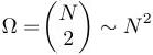
- If System S has energy
 , that leaves of energy for the reservoir. The reservoir must therefore be in a state with 999 0-energy atoms and 1 -energy atoms. That one excited atom could be any of the 1000 atoms, so that’s 1000 microstates.
 - If System S has energy
 , that leaves no energy for the reservoir. The reservoir must therefore be in a state with all of its atoms in their ground states, which is only one possible microstate.
Condensation in a Two-State System Part 2
The difference is in the degeneracy.
- At
 (all particles in the ground state) both the system of bosons and the system of distinguishable particles have a degeneracy of 1.
 - For
 , one excited particle, the boson system has
  and the distinguishable particle system has Ω=N.
 - For
 the boson system still has . (That never changes, right?) The system of distinguishable particles has:
The Boltzmann factors decrease with increasing energy in exactly the same way for both distinguishable particles and bosons, but for distinguishable particles the growth in degeneracy overwhelms the decrease in that Boltzmann factor.
In order for current to flow from the “High V” lead to the “Low V” lead, it must flow through both [add emphasis to the word ‘both’. Using bold, underline, italic, whatever is available in the template] transistors: first the top one, and then the bottom one. The book chose the convention that a high input voltage to a transistor allows current to flow, while a low voltage blocks current. (Remember that a transistor could easily be made the other way around.) Based on that convention…
- If both transistors have high voltage, current will flow through both; you can think of the entire two-transistor assembly (above the resistor) as just a wire. So the output lead is at the “High V” voltage. In this scenario, the voltage drops from High V to Low V across the resistor.
- But if either (or both) transistor has a low voltage, it blocks the current. Because no current flows through the resistor, both sides of the resistor are at the same potential as each other, so the output lead is at the “Low V” voltage. In this scenario, the voltage drops from High V to Low V across the transistors.
This is therefore a design for an “AND gate”; the output lead is high if, and only if, both input leads are high.
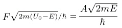
Relativity and Bubble Chambers
1. ![]()
2. ![]()
![]()
3. We have seen that a particle with a lifetime of ![]() (as measured in its own reference frame, which is of course the correct frame for determining when it will decay) would leave a track of
(as measured in its own reference frame, which is of course the correct frame for determining when it will decay) would leave a track of ![]() , which is the shortest track we can currently measure. So any longer lifetime will leave a longer track, and therefore be more easily detectable.
, which is the shortest track we can currently measure. So any longer lifetime will leave a longer track, and therefore be more easily detectable.
1. A baryon is a combination of a red, a blue, and a green quark. Those colors do not impose any restriction on flavor: remember that every flavor of quark (up, charm, etc) can come in all three colors. But we do have to use exactly three quarks to make a baryon. Each quark will have a charge of (2/3)![]() or -(1/3)
or -(1/3)![]() . (They cannot have the opposites of those charges, because then they would be antiquarks, and they would make an antibaryon.) Since we want the total charge to be -1, we want all three quarks to have charge -(1/3)
. (They cannot have the opposites of those charges, because then they would be antiquarks, and they would make an antibaryon.) Since we want the total charge to be -1, we want all three quarks to have charge -(1/3)![]() . The lightest [add emphasis to the word ‘lightest’. Using bold, underline, italic, whatever is available in the template] way to achieve that is to choose all three of our quarks from the left-most (lightest) family.
. The lightest [add emphasis to the word ‘lightest’. Using bold, underline, italic, whatever is available in the template] way to achieve that is to choose all three of our quarks from the left-most (lightest) family.
So the answer is: three down quarks, one of each color.
2. A meson is a combination of a quark (charge (2/3)![]() or -(1/3)
or -(1/3)![]() ) and an antiquark (charge -(2/3)
) and an antiquark (charge -(2/3)![]() or (1/3)
or (1/3)![]() ) with complementary colors. Since we once again want the lighest possible combination, we once again go to the left-most family and combine a down (charge -(1/3)
) with complementary colors. Since we once again want the lighest possible combination, we once again go to the left-most family and combine a down (charge -(1/3)![]() ) with an antiup (charge -(2/3)
) with an antiup (charge -(2/3)![]() ). The colors must match: for instance, if the former is blue, the latter must be antiblue.
). The colors must match: for instance, if the former is blue, the latter must be antiblue.
- Perhaps the biggest limitation of the analogy is that water tends to reduce an object’s velocity; the Higgs field (or mass) reduces acceleration. Those two effects look very similar when you’re trying to speed something up. Push on a still block under water, and the water makes it harder to get the block moving. Push on a very massive object in outer space, and its high mass makes it harder to get the object moving. That’s why the analogy works at all.
But if a block is already moving through water, the water tends to slow it down. If a massive object is already moving through space, its large mass makes it harder to slow. So now the analogy works backward!
Of course, the whole distinction between “speeding up an object” and “slowing down an object” in outer space is reference frame dependent. Water picks out one particular reference frame, and slows everything down relative to that frame. The Higgs field does not establish a preferred reference frame.
- Another limitation of the analogy is that mass—and therefore the Higgs field—actually has two very different effects. One effect is inertia (a larger object is harder to accelerate, as discussed above). The second effect is gravity: a larger object creates, and experiences, a greater gravitational force. This second effect is not reflected in the water analogy.
- Finally, note that water does not create an object’s inertia; it only increases it. Move the object into the air and it becomes easier to move; put it in outer space, and it is still easier. But no matter where you put it, the object still has some mass, and responds to a force with a finite acceleration. Without the Higgs field, all objects would be literally massless!
You can make arbitrarily many diagrams for this process by adding more charged particle loops inside any photon line, as we did in our example.
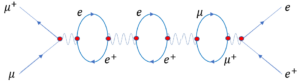
You can also have any charged particle emit and absorb a photon.
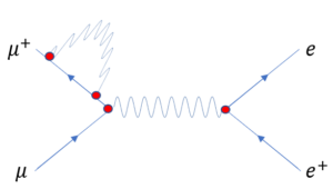
And you can mix and match these in any way, including having one charged particle emit a photon and having a different one absorb it.
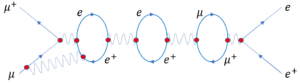
The key is that whenever lines come together there are two straight lines (representing the same kind of particle) and one wavy line, and the only lines that don’t start and end inside the diagram are the initial muon/antimuon pair and the final electron/positron pair.
Light Beams in an Expanding Universe
Remember that, because ![]() is on the vertical axis, a lower velocity is indicated by a steeper slope.
is on the vertical axis, a lower velocity is indicated by a steeper slope.