

1 Introduction
Science is more than a collection of observed associations. While the description and cataloging of phenomena play a role in scientific discovery, the ultimate goal of science is the amalgamation of theories that have survived rigorous falsification (Reference Hassani, Huang and GhodsiHassani et al. 2018). For a theory to be scientific, it is generally expected to declare the falsifiable causal mechanism responsible for the observed phenomenon (for one definition of falsifiability, see Reference PopperPopper 1963).Footnote 1 Put simply, a scientific theory explains why an observed phenomenon takes place, where that explanation is consistent with all the empirical evidence (ideally, including experimental results). Economists subscribe to this view that a genuine science must produce refutable implications, and that those implications must be tested through solid statistical techniques (Reference LazearLazear 2000).
In the experimental sciences (physics, chemistry, biology, etc.), it is relatively straightforward to propose and falsify causal mechanisms through interventional studies (Reference FisherFisher 1971). This is not generally the case in financial economics. Researchers cannot reproduce the financial conditions of the Flash Crash of May 6, 2010, remove some traders, and observe whether stock market prices still collapse. This has placed the field of financial economics at a disadvantage when compared with experimental sciences. A direct consequence of this limitation is that, for the past fifty years, most factor investing researchers have focused on publishing associational claims, without theorizing and subjecting to falsification the causal mechanisms responsible for the observed associations. In the absence of plausible falsifiable theories, researchers must acknowledge that they do not understand why the reported anomalies (risk premia) occur, and investors are entitled to dismiss their claims as spurious. The implication is that the factor investing literature remains in an immature, phenomenological stage.
From the above, one may reach the bleak conclusion that there is no hope for factor investing (or financial economics) to produce and build upon scientific theories. This is not necessarily the case. Financial economics is not the only field of study afflicted by barriers to experimentation (e.g., astronomers produce scientific theories despite the unfeasibility of interventional studies). Recent progress in causal inference has opened a path, however difficult, for advancing factor investing beyond its current phenomenological stage. The goal of this Element is to help factor investing wake up from its associational slumber, and plant the seeds for the new field of “causal factor investing.”
In order to achieve this goal, I must first recite the fundamental differences between association and causation (Section 2), and why the study of association alone does not lead to scientific knowledge (Section 3). In fields of research with barriers to experimentation, like investing, it has become possible to estimate causal effects from observational studies, through natural experiments and simulated interventions (Section 4). After laying out this foundation, I turn the reader’s attention to the current state of causal confusion in econometrics (Section 5) and factor investing studies (Section 6). This state of confusion easily explains why factor investing remains in a phenomenological stage, and the proliferation of hundreds of spurious claims that Reference CochraneCochrane (2011) vividly described as the “factor zoo”Footnote 2 (Section 7). The good news is, once financial economists embrace the concepts described in this Element, I foresee the transformation of factor investing into a truly scientific discipline (Section 8).
This Element makes several contributions. First, I describe the logical inconsistency that afflicts the factor investing literature, whereby authors make associational claims in denial or ignorance of the causal content of their models. Second, I define the two different types of spurious claims in factor investing, type-A and type-B. These two types of spurious claims have different origins and consequences, hence it is important for factor researchers to distinguish between the two. In particular, type-B factor spuriosity is an important topic that has not been discussed in depth until now. Type-B spuriosity explains, among other literature findings, the time-varying nature of risk premia. Third, I apply this taxonomy to derive a hierarchy of empirical evidence used in financial research, based on the evidence’s susceptibility to being spurious. Fourth, I design Monte Carlo experiments that illustrate the dire consequences of type-B spurious claims in factor investing. Fifth, I propose an alternative explanation for the main findings of the factor investing literature, which is consistent with type-B spuriosity. In particular, the time-varying nature of risk premia reported in canonical journal articles is a likely consequence of under-controlling. Sixth, I propose specific actions that academic authors can take to rebuild factor investing on the more solid scientific foundations of causal inference.
2 Association vs Causation
Every student of statistics, and by extension econometrics, learns that association does not imply causation. This statement, while superficially true, does not explain why association exists, and its relation to causation. Two discrete random variables X and Y are statistically independent if and only if
 , where
 is the probability of the event described inside the squared brackets. Conversely, two discrete random variables
 and
and
 are said to be statistically associated (or codependent) when, for some
 , they satisfy that
 . The conditional probability expression
 represents the probability that
 among the subset of the population where
 . When two variables are associated, observing the value of one conveys information about the value of the other:
 , or equivalently,
 . For example, monthly drownings (
 ) and ice cream sales (
 ) are strongly associated, because the probability that
 people drown in a month conditional on observing
 ice cream sales in that same month does not equal the unconditional probability of
 drownings in a month for some
 . However, the expression
 does not tell us whether ice cream sales cause drownings. Answering that question requires the introduction of a more nuanced concept than conditional probability: an intervention.
A data-generating process is a physical process responsible for generating the observed data, where the process is characterized by a system of structural equations. Within that system, a variable
 is said to cause a variable
 when
when
 is a function of
 . The structural equation by which
 causes
 is called a causal mechanism. Unfortunately, the data-generating process responsible for observations is rarely known. Instead, researchers must rely on probabilities, estimated on a sample of observations, to deduce the causal structure of a system. Probabilistically, a variable
 is said to cause a variable
 when setting the value of
 to
to
 increases the likelihood that
 will take the value
 . Econometrics lacks the language to represent interventions, that is, setting the value of
 (Reference Chen and PearlChen and Pearl 2013). To avoid confusion between conditioning by
 and setting the value of
 , Reference PearlPearl (1995) introduced the do-operator,
 , which denotes the intervention that sets the value of
 to
to
 . With this new notation, causation can be formally defined as follows:
 causes
 if and only if
 .Footnote 3 For example, setting ice cream sales to
 will not make
 drownings more likely than its unconditional probability for any pair
 , hence ice cream sales are not a cause of drownings. In contrast, smoking tobacco is a cause of lung cancer, because the probability that
 individuals develop lung cancer among a collective where the level of tobacco smoking is set to
 (through an intervention) is greater than the unconditional probability of
 individuals developing lung cancer, for some pair
 .Footnote 4
Variables
 and
and
 may be part of a more complex system, involving additional variables. The causal structure of a system can be represented through a directed acyclic graph, also denoted a causal graph.Footnote 5 While a causal graph does not fully characterize the data-generating process, it conveys topological information essential to estimate causal effects. Causal graphs declare the variables involved in a system, which variables influence each other, and the direction of causality (Reference PearlPearl 2009, p. 12). Causal graphs help visualize do-operations as the action of removing all arrows pointing toward
 in the causal graph, so that the full effect on
 can be attributed to setting
 . This is the meaning of the ceteris paribus assumption, which is of critical importance to economists.
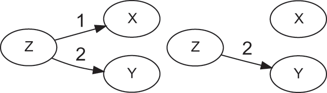
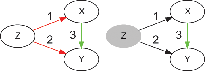
The causal graph in Figure 1 tells us that
 causes
 , and
, and
 causes
 . In the language of causal inference,
 is a confounder, because this variable introduces an association between
 and
and
 , even though there is no arrow between
 and
and
 . For this reason, this type of association is denoted noncausal. Following with the previous example, weather (
 ) influences ice cream sales (
 ) and the number of swimmers, hence drownings (
 ). The intervention that sets ice cream sales removes arrow (1), because it gives full control of
 to the researcher (
 is no longer a function of
 ), while keeping all other things equal (literally, ceteris paribus). And because
 does not cause
 , setting
 (e.g., banning the sale of ice cream,
 ) has no effect on the probability of
 . As shown later, noncausal association can occur for a variety of additional reasons that do not involve confounders.
Causal graph of a confounder (
 ), before (left) and after (right) a do-operation
Five conclusions can be derived from this exposition. First, causality is an extra-statistical (in the sense of beyond observational) concept, connected to mechanisms and interventions, and distinct from the concept of association. As a consequence, researchers cannot describe causal systems with the associational language of conditional probabilities. Failure to use the do-operator has led to confusion between associational and causal statements, in econometrics and elsewhere. Second, association does not imply causation, however causation does imply association because setting
 through an intervention is associated with the outcome
 .Footnote 6 Third, unlike association, causality is directional, as represented by the arrows of the causal graph. The statement “
 causes
 ” implies that
 , but not that
 . Fourth, unlike association, causality is sequential. “
 causes
 ” implies that the value of
 is set first, and only after that
 adapts. Fifth, the ceteris paribus assumption simulates an intervention (do-operation), whose implications can only be understood with knowledge of the causal graph. The causal graph shows what “other things” are kept equal by the intervention.
3 The Three Steps of Scientific Discovery
Knowing the causes of effects has long been a human aspiration. In 29 BC, ancient Roman poet Virgil wrote “happy the man, who, studying Nature’s laws, / thro’ known effects can trace the secret cause” (Reference DrydenDryden 1697, p. 71). It was not until around the year 1011 that Arab mathematician Hasan Ibn al-Haytham proposed a scientific method for deducing the causes of effects (Reference ThieleThiele 2005; Reference SabraSabra 1989).
Science has been defined as the systematic organization of knowledge in the form of testable explanations of natural observations (Reference HeilbronHeilbron 2003). Mature scientific knowledge aims at identifying causal relations, and the mechanisms behind them, because causal relations are responsible for the regularities in observed data (Reference Glymour, Zhang and SpirtesGlymour et al. 2019).
The process of creating scientific knowledge can be organized around three critical steps: (1) the phenomenological step, where researchers observe a recurrent pattern of associated events, or an exception to such a pattern; (2) the theoretical step, where researchers propose a testable causal mechanism responsible for the observed pattern; and (3) the falsification step, where the research community designs experiments aimed at falsifying each component of the theorized causal mechanism.
3.1 The Phenomenological Step
In the phenomenological step, researchers observe associated events, without exploring the reason for that association. At this step, it suffices to discover that
 . Further, a researcher may model the joint distribution
 , derive conditional probabilities
 , and make associational statements of the type
 (an associational prediction) with the help of machine learning tools. Exceptionally, a researcher may go as far as to produce empirical evidence of a causal effect, such as the result from an interventional study (e.g., Ohm’s law of current, Newton’s law of universal gravitation, or Coulomb’s law of electrical forces), but without providing an explanation for the relationship. The main goal of the phenomenological step is to state “a problem situation,” in the sense of describing the observed anomaly for which no scientific explanation exists (Reference PopperPopper 1994b, pp. 2–3). At this step, inference occurs by logical induction, because the problem situation rests on the conclusion that, for some unknown reason, the phenomenon will reoccur.Footnote 7
For instance, a researcher may observe that the bid-ask spread of stocks widens in the presence of imbalanced orderflow (i.e., when the amount of shares exchanged in trades initiated by buyers does not equal the amount of shares exchanged in trades initiated by sellers over a period of time), and that the widening of bid-ask spreads often precedes a rise in intraday volatility. This is a surprising phenomenon because under the efficient market hypothesis asset prices are expected to reflect all available information at all times, making predictions futile (Reference FamaFama 1970). The existence of orderflow imbalance, the sequential nature of these events, and their predictability point to market inefficiencies, of unclear source. Such associational observations do not constitute a theory, and they do not explain why the phenomenon occurs.
3.2 The Theoretical Step
In the theoretical step, researchers advance a possible explanation for the observed associated events. This is an exercise in logical abduction (sometimes also called retroduction): Given the observed phenomenon, the most likely explanation is inferred by elimination among competing alternatives. Observations cannot be explained by a hypothesis more extraordinary than the observations themselves, and of various hypotheses the least extraordinary must be preferred (Reference Wieten, Bex, Prakken, Renooij, Prakken, Bistarelli, Santini and TaticchiWieten et al. 2020). At this step, a researcher states that
 and
and
 are associated because
 causes
 , in the sense that
 . For the explanation to be scientific, it must propose a causal mechanism that is falsifiable, that is, propose the system of structural equations along the causal path from
 to
to
 , where the validity of each causal link and causal path can be tested empirically.Footnote 8 Physics Nobel Prize laureate Wolfgang Pauli famously remarked that there are three types of explanations: correct, wrong, and not even wrong (Reference PeierlsPeierls 1992). With “not even wrong,” Pauli referred to explanations that appear to be scientific, but use unfalsifiable premises or reasoning, which can never be affirmed nor denied.
A scientist may propose a theory with the assistance of statistical tools (see Section 4.3.1), however data and statistical tools are not enough to produce a theory. The reason is, in the theoretical step the scientist injects extra-statistical information, in the form of a subjective framework of assumptions that give meaning to the observations. These assumptions are unavoidable, because the simple action of taking and interpreting measurements introduces subjective choices, making the process of discovery a creative endeavor. If theories could be deduced directly from observations, then there would be no need for experiments that test the validity of the assumptions.
Following on the previous example, the Probability of Informed Trading (PIN) theory explains liquidity provision as the result of a sequential strategic game between market makers and informed traders (Reference Easley, Kiefer, O’Hara and PapermanEasley et al. 1996). In the absence of informed traders, the orderflow is balanced, because uninformed traders initiate buys and sells in roughly equal amounts, hence market impact is mute and the mid-price barely changes. When market makers provide liquidity to uninformed traders, they profit from the bid-ask spread (they buy at the bid price and sell at the ask price). However, the presence of informed traders imbalances the orderflow, creating market impact that changes the mid-price. When market makers provide liquidity to an informed trader, the mid-price changes before market makers are able to profit from the bid-ask spread, and they are eventually forced to realize a loss. As a protection against losses, market makers react to orderflow imbalance by charging a greater premium for selling the option to be adversely selected (that premium is the bid-ask spread). In the presence of persistent orderflow imbalance, realized losses accumulate, and market makers are forced to reduce their provision of liquidity, which results in greater volatility. Two features make the PIN theory scientific: First, it describes a precise mechanism that explains the causal link: orderflow imbalance
 market impact
 mid-price change
 realized losses
 bid-ask spread widening
 reduced liquidity
 greater volatility. Second, the mechanism involves measurable variables, with links that are individually testable. An unscientific explanation would not propose a mechanism, or it would propose a mechanism that is not testable.
Mathematicians use the term theory with a different meaning than scientists. A mathematical theory is an area of study derived from a set of axioms, such as number theory or group theory. Following Kant’s epistemological definitions, mathematical theories are synthetic a priori logical statements, whereas scientific theories are synthetic a posteriori logical statements. This means that mathematical theories do not admit empirical evidence to the contrary, whereas scientific theories must open themselves to falsification.
3.3 The Falsification Step
In the falsification step, researchers not involved in the formulation of the theory independently: (i) deduce key implications from the theory, such that it is impossible for the theory to be true and the implications to be false; and (ii) design and execute experiments with the purpose of proving that the implications are false. Step (i) is an exercise in logical deduction because given some theorized premises, a falsifiable conclusion is reached reductively (Reference GenslerGensler 2010, pp. 104–110). When properly done, performing step (i) demands substantial creativity and domain expertise, as it must balance the strength of the deduced implication with its testability (cost, measurement errors, reproducibility, etc.). Each experiment in step (ii) focuses on falsifying one particular link in the chain of events involved in the causal mechanism, applying the tools of mediation analysis. The conclusion that the theory is false follows the structure of a modus tollens syllogism (proof by contradiction): using standard sequent notation, if
 , however
 is observed, then
 , where
 stands for “the theory is true” and
 stands for a falsifiable key implication of the theory.
One strategy of falsification is to show that
 , in which case either the association is noncausal, or there is no association (i.e., the phenomenon originally observed in step (i) was a statistical fluke). A second strategy of falsification is to deduce a causal prediction from the proposed mechanism, and to show that
 . When that is the case, there may be a causal mechanism, however, it does not work as theorized (e.g., when the actual causal graph is more complex than the one proposed). A third strategy of falsification is to deduce from the theorized causal mechanism the existence of associations, and then apply machine learning techniques to show that those associations do not exist. Unlike the first two falsification strategies, the third one does not involve a do-operation.
Following on the previous example, a researcher may split a list of stocks randomly into two groups, send buy orders that set the level of orderflow imbalance for the first group, and measure the difference in bid-ask spread, liquidity, and volatility between the two groups (an interventional study, see Section 4.1).Footnote 9 In response to random spikes in orderflow imbalance, a researcher may find evidence of quote cancellation, quote size reduction, and resending quotes further away from the mid-price (a natural experiment, see Section 4.2).Footnote 10 If the experimental evidence is consistent with the proposed PIN theory, the research community concludes that the theory has (temporarily) survived falsification. Furthermore, in some cases a researcher might be able to inspect the data-generating process directly, in what I call a “field study.” A researcher may approach profitable market makers and examine whether their liquidity provision algorithms are designed to widen the bid-ask spread at which they place quotes when they observe imbalanced order flow. The same researcher may approach less profitable market makers and examine whether their liquidity provision algorithms do not react to order flow imbalance. Service providers are willing to offer this level of disclosure to key clients and regulators. This field study may confirm that market makers who do not adjust their bid-ask spread in presence of orderflow imbalance succumb to Darwinian competition, leaving as survivors those whose behavior aligns with the PIN theory.
Popper gave special significance to falsification through “risky forecasts,” that is, forecasts of outcomes
 under yet unobserved interventions
 (Reference Vignero and WenmackersVignero and Wenmackers 2021). Mathematically, this type of falsification is represented by the counterfactual expression
 , namely the expected value of
 in an alternative universe where
 is set to
 (a do-operation) for the subset of observations where what actually happened is
 and
and
 .Footnote 11 Successful theories answer questions about previously observed events, as well as never-before observed events. To come up with risky forecasts, an experiment designer scrutinizes the theory, deducing its ultimate implications under hypothetical
 , and then searches or waits for them. Because the theory was developed during the theoretical step without knowledge of
 , this type of analysis constitutes an instance of out-of-sample assessment. For example, the PIN theory implied the possibility of failures in the provision of liquidity approximately fourteen years before the flash crash of 2010 took place. Traders who had implemented liquidity provision models based on the PIN theory (or better, its high-frequency embodiment, VPIN) were prepared for that black-swan and profited from that event (Reference Easley, Prado and O’HaraEasley et al. 2010, Reference Easley, Prado and O’Hara2012, Reference López de PradoLópez de Prado 2018, pp. 281–300), at the expense of traders who relied on weaker microstructural theories.
3.4 Demarcation and Falsificationism in Statistics
Science is essential to human understanding in that it replaces unreliable inductive reasoning (such as “
 will follow
 because that is the association observed in the past”) with more reliable deductive reasoning (such as “
 will follow
 because
 causes
 through a tested mechanism
 ”). Parsimonious theories are preferable, because they are easier to falsify, as they involve controlling for fewer variables (Occam’s razor). The most parsimonious surviving theory is not truer, however, it is better “fit” (in an evolutionary sense) to tackle more difficult problems posed by that theory. The most parsimonious surviving theory poses new problem situations, hence re-starting a new iteration of the three-step process, which will result in a better theory yet.
To appreciate the unique characteristics of the scientific method, it helps to contrast it with a dialectical predecessor. For centuries prior to the scientific revolution of the seventeenth century, academics used the Socratic method to eliminate logically inconsistent hypotheses. Like the scientific method, the Socratic method relies on three steps: (1) problem statement; (2) hypothesis formulation; and (3) elenchus (refutation), see Reference VlastosVlastos (1983, pp. 27–58). However, both methods differ in three important aspects. First, a Socratic problem statement is a definiendum (“what is
 ?”), not an observed empirical phenomenon (“
 and
and
 are associated”). Second, a Socratic hypothesis is a definiens (“
 is …”), not a falsifiable theory (“
 causes
 through mechanism
 ”). Third, a Socratic refutation presents a counterexample that exposes implicit assumptions, where those assumptions contradict the original definition. In contrast, scientific falsification does not involve searching for contradictive implicit assumptions, since all assumptions were made explicit and coherent by a plausible causal mechanism. Instead, scientific falsification designs and executes an experiment aimed at debunking the theorized causal effect (“
 does not cause
 ”), or showing that the experiment’s results contradict the hypothesized mechanism (“experimental results contradict
 ”).Footnote 12
The above explanation elucidates an important fact that is often ignored or misunderstood: not all academic debate is scientific, even in empirical or mathematical subjects. A claim does not become scientific by virtue of its use of complex mathematics, its reliance on measurements, or its submission to peer review.Footnote 13 Philosophers of science call the challenge of separating scientific claims from pseudoscientific claims the “demarcation problem.” Popper, Kuhn, Lakatos, Musgrave, Thagard, Laudan, Lutz, and many other authors have proposed different demarcation principles. While there is no consensus on what constitutes a definitive demarcation principle across all disciplines, modern philosophers of science generally agree that, for a theory to be scientific, it must be falsifiable in some wide or narrow sense.Footnote 14
The principle of falsification is deeply ingrained in statistics and econometrics (Reference Dickson, Baird, Bandyopadhyay and ForsterDickson and Baird 2011). Frequentist statisticians routinely use Fisher’s p-values and Neyman–Pearson’s framework for falsifying a proposed hypothesis (
 ), following a hypothetico-deductive argument of the form (using standard sequent notation):
 (1)
(1)
where
 denotes the observation made and
 denotes the targeted false positive rate (Reference PerezgonzalezPerezgonzalez 2017). The above proposition is analogous to a modus tollens syllogism, with the caveat that
 is not rejected with certainty, as it would be the case in a mathematical proof. For this reason, this proposition is categorized as a stochastic proof by contradiction, where certainty is replaced by a preset confidence level (Reference ImaiImai 2013; Reference Balsubramani and RamdasBalsubramani and Ramdas 2016). Failure to reject
 does not validate
 , but rather attests that there is not sufficient empirical evidence to cast significant doubt on the truth of
 (Reference Reeves and BrewerReeves and Brewer 1980).Footnote 15 Accordingly, the logical structure of statistical hypothesis testing enforces a Popperian view of science in quantitative disciplines, whereby a hypothesis can never be accepted, but it can be rejected (i.e., falsified), see Wilkinson (2013). Popper’s influence is also palpable in Bayesian statistics, see Reference Gelman and Rohilla-ShaliziGelman and Rohilla-Shalizi (2013).
Statistical falsification can be applied to different types of claims. For the purpose of this Element, it is helpful to differentiate between the statistical falsification of: (a) associational claims; and (b) causal claims. The statistical falsification of associational claims occurs during the phenomenological step of the scientific method (e.g., when a researcher finds that “
 is correlated with
 ”), and it can be done on the sole basis of observational evidence. The statistical falsification of causal claims may also occur at the phenomenological step of the scientific method (e.g., when a laboratory finds that “
 causes
 ” in the absence of any theory to explain why), or at the falsification step of the scientific method (involving a theory, of the form “
 causes
 through a mechanism
 ”), but either way the statistical falsification of a causal claim always requires an experiment.Footnote 16 Most statisticians and econometricians are trained in the statistical falsification of associational claims and have a limited understanding of the statistical falsification of causal claims in general, and the statistical falsification of causal theories in particular. The statistical falsification of causal claims requires the careful design of experiments, and the statistical falsification of causal theories requires testing the hypothesized causal mechanism, which in turn requires testing independent effects along the causal path. The next section delves into this important topic.
4 Causal Inference
The academic field of causal inference studies methods to determine the independent effect of a particular variable within a larger system. Assessing independent effects is far from trivial, as the fundamental problem of causal inference illustrates.
Consider two random variables
 , where a researcher wishes to estimate the effect of
 on
on
 . Let
. Let
 denote the expected outcome of
 when
when
 is set to
 (control), and let
 denote the expected outcome of
 when
when
 is set to
 (treatment). The average treatment effect (ATE) of
 on
on
 is defined as
 (2)
(2)
In general, ATE is not equal to the observed difference,
 . The observed difference between two states of
 is
is
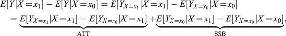 (3)
(3)
where
 is a counterfactual expression, representing the expected value of
 in an alternative universe where
 is set to
 , given that what actually happened is
 . Naturally,
 , for
, for
 , because the counterfactual expression (the left-hand side) replicates what actually happened (right-hand side).
The above equation splits the observed difference into two components, the so-called average treatment effect on the treated (ATT) and self-selection bias (SSB). The fundamental problem of causal inference is that computing ATT requires estimating the counterfactual
 , which is not directly observable. What is directly observable is the difference
 , however that estimand of ATT is biased by SSB. The impact of SSB on
 can be significant, to the point of misleading the researcher. Following the earlier example, suppose that
 is the number of drownings in a month,
 represents low ice cream monthly sales, and
 represents high ice cream monthly sales. The value of
 is high, because of the confounding effect of warm weather, which encourages both, ice cream sales and swimming. While high ice cream sales are associated with more drownings, it would be incorrect to infer that the former is a cause of the latter. The counterfactual
 represents the expected number of drownings in a month of high ice cream sales, should ice cream sales have been suppressed. The value of that unobserved counterfactual is arguably close to the observed
 , hence
 , and the observed difference is largely due to SSB.
Studies designed to establish causality propose methods to nullify SSB. These studies can be largely grouped into three types: interventional studies, natural experiments, and simulated interventions.
4.1 Interventional Studies
In a controlled experiment, scientists assess causality by observing the effect on
 of changing the values of
 while keeping constant all other variables in the system (a do-operation). Hasan Ibn al-Haytham (965–1040) conducted the first recorded controlled experiment in history, in which he designed a camera obscura to manipulate variables involved in vision. Through various ingenious experiments, Ibn al-Haytham showed that light travels in a straight line, and that light reflects from the observed objects to the observer’s eyes, hence falsifying the extramission theories of light by Ptolemy, Galen, and Euclid (Reference ToomerToomer 1964). This example illustrates a strong prerequisite for conducting a controlled experiment: the researcher must have direct control of all the variables involved in the data-generating process. When that is the case, the ceteris paribus condition is satisfied, and the difference in
 can be attributed to the change in
 .
.
When some of the variables in the data-generating process are not under direct experimental control (e.g., the weather in the drownings example), the ceteris paribus condition cannot be guaranteed. In that case, scientists may execute a randomized controlled trial (RCT), whereby members of a population (called units or subjects) are randomly assigned either to a treatment or to a control group. Such random assignment aims to create two groups that are as comparable as possible, so that any difference in outcomes can be attributed to the treatment. In an RCT, the researcher carries out the do-operation on two random samples of units, rather than on a particular unit, hence enabling a ceteris paribus comparison. The randomization also allows the researcher to quantify the experiment’s uncertainty via Monte Carlo, by computing the standard deviation on ATEs from different subsamples. Scientists may keep secret from participants (single-blind) and researchers (double-blind) which units belong to each group, in order to further remove subject and experimenter biases. For additional information, see Reference Hernán and RobinsHernán and Robins (2020) and Reference Kohavi, Tang, Xu, Hemkens and IoannidisKohavi et al. (2020).
We can use the earlier characterization of the fundamental problem of causal inference to show how random assignment achieves its goal. Consider the situation where a researcher assigns units randomly to
 (control group) and
 (treatment group). Following with the earlier example, this is equivalent to tossing a coin at the beginning of every month, then setting
 (low ice cream sales) on heads and setting
 (high ice cream sales) on tails. Because the intervention on
 was decided at random, units in the treatment group are expected to be undistinguishable from units in the control group, hence
 (4)
(4)
 (5)
(5)
Random assignment makes
 and
and
 independent of the observed
 . The implication from the first equation above is that
 . In the drownings example,
 , because suppressing ice cream sales would have had the same expected outcome (
 ) on both, high sales months and low sales months, since the monthly sales were set at random to begin with (irrespective of the weather).
In conclusion, under random assignment, the observed difference matches both ATT and ATE:
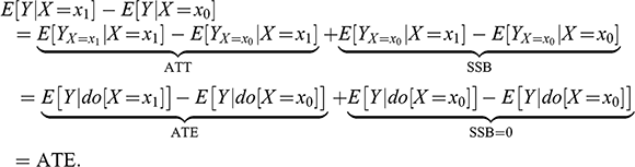 (6)
(6)
4.2 Natural Experiments
Sometimes interventional studies are not possible, because they are unfeasible, unethical, or prohibitively expensive. Under those circumstances, scientists may resort to natural experiments or simulated interventions. In a natural experiment (also known as a quasi-experiment), units are assigned to the treatment and control groups determined randomly by Nature or by other factors outside the influence of scientists (Reference DunningDunning 2012). Although natural experiments are observational (as opposed to interventional, like controlled experiments and RCT) studies, the fact that the assignment of units to groups is assumed random enables the attribution of the difference in outcomes to the treatment. Put differently, Nature performs the do-operation, and the researcher’s challenge is to identify the two random groups that enable a ceteris paribus comparison. Common examples of natural experiments include (1) regression discontinuity design (RDD); (2) crossover studies (COSs); and (3) difference-in-differences (DID) studies. Case–control studies,Footnote 17 cohort studies,Footnote 18 and synthetic control studiesFootnote 19 are not proper natural experiments because there is no random assignment of units to groups.
Regression discontinuity design studies compare the outcomes of: (a) units that received treatment because the value of an assignment variable fell barely above a threshold; and (b) units that escaped treatment because the value of an assignment variable fell barely below a threshold. The critical assumption behind RDD is that groups (a) and (b) are comparable in everything but the slight difference in the assignment variable, which can be attributed to noise, hence the difference in outcomes between (a) and (b) is the treatment effect. For further reading, see Reference Imbens and LemieuxImbens and Lemieux (2008).
A COS is a longitudinal study in which the exposure of units to a treatment is randomly removed for a time, and then returned. COS assumes that the effect of confounders does not change per unit over time. When that assumption holds, COSs have two advantages over standard longitudinal studies. First, in a COS the influence of confounding variables is reduced by each unit serving as its own control. Second, COS are statistically efficient, as they can identify causal effects in smaller samples than other studies. COS may not be appropriate when the order of treatments affects the outcome (order effects). Sufficiently long wash-out periods should be observed between treatments, to avoid that past treatments confound the estimated effects of new treatments (carryover effects). COS can also have an interventional counterpart, when the random assignment is under the control of the researcher. To learn more, see Reference Jones and KenwardJones and Kenward (2003).
When factors other than the treatment influence the outcome over time, researchers may apply a pre-post with-without comparison, called a DID study. In a DID study, researchers compare two differences: (i) the before-after difference in outcomes of the treatment group; and (ii) the before-after difference in outcomes of the control group (where the random assignment of units to groups is done by Nature). By computing the difference between (i) and (ii), DID attempts to remove from the treatment effect (i) all time-varying factors captured by (ii). DID relies on the “equal-trends assumption,” namely that no time-varying differences exist between treatment and control groups. The validity of the equal-trends assumption can be assessed in a number of ways. For example, researchers may compute changes in outcomes for the treatment and control groups repeatedly before the treatment is actually administered, so as to confirm that the outcome trends move in parallel. For additional information, see Reference Angrist and PischkeAngrist and Pischke (2008, pp. 227–243).
4.3 Simulated Interventions
The previous sections explained how interventional studies and natural experiments use randomization to achieve the ceteris paribus comparisons that result in
 . Each approach demanded stronger assumptions than the previous one, with the corresponding cost in terms of generality of the conclusions. For instance, the conclusions from a controlled experiment are more general than the conclusions from an RCT, because in the former researchers control the variables involved in the data-generating process in such a way that ceteris paribus comparisons are clearer. Likewise, the conclusions from an RCT are more general than the conclusions from a natural experiment, because in an RCT the researcher is in control of the random assignment, and the researcher performs the do-operation.
In recent decades, the field of causal inference has added one more tool to the scientific arsenal: when interventional studies and natural experiments are not possible, researchers may still conduct an observational study that simulates a do-operation, with the help of a hypothesized causal graph. The hypothesized causal graph encodes the information needed to remove from observations the SSB introduced by confounders, under the assumption that the causal graph is correct. The price to pay is, as one might have expected, accepting stronger assumptions that make the conclusions less general, but still useful.
Simulated interventions have two main applications: First, subject to a hypothesized causal graph, a simulated intervention allows researchers to estimate the strength of a causal effect from observational studies. Second, a simulated intervention may help falsify a hypothesized causal graph, when the strength of one of the effects posited by the graph is deemed statistically insignificant (once again, a modus tollens argument, see Section 3.4).
It is important to understand the difference between establishing a causal claim and falsifying a causal claim. Through interventional studies and natural experiments, subject to some assumptions, a researcher can establish or falsify a causal claim without knowledge of the causal graph. For this reason, they are the most powerful tools in causal inference. In simulated interventions, the causal graph is part of the assumptions, and one cannot prove what one is assuming. The most a simulated intervention can achieve is to disprove a hypothesized causal graph, by finding a contradiction between an effect claimed by a graph and the effect estimated with the help of that same graph. This power of simulated interventions to falsify causal claims can be very helpful in discovering through elimination the causal structure hidden in the data.
4.3.1 Causal Discovery
Causal discovery can be defined as the search for the structure of causal relationships, by analyzing the statistical properties of observational evidence (Reference Spirtes, Glymour and ScheinesSpirtes et al. 2001). While observational evidence almost never suffices to fully characterize a causal graph, it often contains information helpful in reducing the number of possible structures of interdependence among variables. At the very least, the extra-statistical information assumed by the causal graph should be compatible with the observations. Over the past three decades, statisticians have developed numerous computational methods and algorithms for the discovery of causal relations, represented as directed acyclic graphs (see Reference Glymour, Zhang and SpirtesGlymour et al. 2019). These methods can be divided into the following classes: (a) constraint-based algorithms; (b) score-based algorithms; and (c) functional causal models (FCMs).
Constraint-based methods exploit conditional independence relationships in the data to recover the underlying causal structure. Two of the most widely used methods are the PC algorithm (named after its authors, Peter Spirtes and Clark Glymour), and the fast causal inference (FCI) algorithm (Reference Spirtes, Glymour and ScheinesSpirtes et al. 2000). The PC algorithm assumes that there are no latent (unobservable) confounders, and under this assumption the discovered causal information is asymptotically correct. The FCI algorithm gives asymptotically correct results even in the presence of latent confounders.
Score-based methods can be used in the absence of latent confounders. These algorithms attempt to find the causal structure by optimizing a defined score function. An example of a score-based method is the greedy equivalence search (GES) algorithm. This heuristic algorithm searches over the space of Markov equivalence classes, that is, the set of causal structures satisfying the same conditional independences, evaluating the fitness of each structure based on a score calculated from the data (Reference ChickeringChickering 2003). The GES algorithm is known to be consistent under certain assumptions, which means that as the sample size increases, the algorithm will converge to the true causal structure with probability approaching 1. However, this does not necessarily mean that the algorithm will converge to the true causal structure in finite time or with a reasonable sample size. GES is also known to be sensitive to the initial ordering of variables.
FCMs distinguish between different directed-acyclic graphs in the same equivalence class. This comes at the cost of making additional assumptions on the data distribution than conditional independence relations. A FCM models the effect variable
 as
as
 , where
 is a function of the direct causes
 and
and
 is noise that is independent of
 . Subject to the aforementioned assumptions, the causal direction between
 and
and
 is identifiable, because the independence condition between
 and
and
 holds only for the true causal direction (Reference Shimizu, Hoyer, Hyvärinen and KerminenShimizu et al. 2006; Reference Hoyer, Janzing, Mooji, Peters and SchölkopfHoyer et al. 2009; and Reference Zhang and HyvärinenZhang and Hyvaerinen 2009).
Causal graphs can also be derived from nonnumerical data. For example, Reference Laudy, Denev and GinsbergLaudy et al. (2022) apply natural language processing techniques to news articles in which different authors express views of the form
 . By aggregating those views, these researchers derive directed acyclic graphs that represent collective, forward-looking, point-in-time views of causal mechanisms.
Machine learning is a powerful tool for causal discovery. Various methods allow researchers to identify the important variables associated in a phenomenon, with minimal model specification assumptions. In doing so, these methods decouple the variable search from the specification search, in contrast with traditional statistical methods. Examples include mean-decrease accuracy, local surrogate models, and Shapley values (Reference López de PradoLópez de Prado 2020, pp. 3–4, Reference López de PradoLópez de Prado 2022a). Once the variables relevant to a phenomenon have been isolated, researchers can apply causal discovery methods to propose a causal structure (identify the links between variables, and the direction of the causal arrows).
4.3.2 Do-Calculus
Do-calculus is a complete axiomatic system that allows researchers to estimate do-operators by means of conditional probabilities, where the necessary and sufficient conditioning variables can be determined with the help of the causal graph (Reference Shpitser and PearlShpitser and Pearl 2006). The following sections review some notions of do-calculus needed to understand this Element. I encourage the reader to learn more about these important concepts in Reference PearlPearl (2009), Reference Pearl, Glymour and JewellPearl et al. (2016), and Reference NealNeal (2020).
4.3.2.1 Blocked Paths
In a graph with three variables
 , a variable
 is a confounder with respect to
 and
and
 when the causal relationships include a structure X ← Z → Y. A variable
 is a collider with respect to
 and
and
 when the causal relationships are reversed, that is, X → Z ← Y. A variable
 is a mediator with respect to
 and
and
 when the causal relationships include a structure X → Z → Y.Footnote 20
A path is a sequence of arrows and nodes that connect two variables
 and
and
 , regardless of the direction of causation. A directed path is a path where all arrows point in the same direction. In a directed path that starts in
 and ends in
 ,
,
 is an ancestor of
 , and
, and
 is a descendant of
 . A path between
 and
and
 is blocked if either: (1) the path traverses a collider, and the researcher has not conditioned on that collider or its descendants; or (2) the researcher conditions on a variable in the path between
 and
and
 , where the conditioned variable is not a collider. Association flows along any paths between
 and
and
 that are not blocked. Causal association flows along an unblocked directed path that starts in treatment
 and ends in outcome
 , denoted the causal path. Association implies causation only if all noncausal paths are blocked. This is the deeper explanation of why association does not imply causation, and why causal independence does not imply statistical independence.
Two variables
 and
and
 are d-separated by a (possibly empty) set of variables
 if, upon conditioning on
 , all paths between
 and
and
 are blocked. The set
 d-separates
 and
and
 if and only if
 and
and
 are conditionally independent given
 . For a proof of this statement, see Reference Koller and FriedmanKoller and Friedman (2009, chapter 3). This important result, sometimes called the global Markov condition in Bayesian network theory,Footnote 21 allows researchers to assume that
 , and estimate ATE as
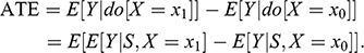 (7)
(7)
The catch is, deciding which variables belong in
 requires knowledge of the causal graph that comprises all the paths between
 and
and
 . Using the above concepts, it is possible to define various specific controls for confounding variables, including: (a) the backdoor adjustment; (b) the front-door adjustment; and (c) the method of instrumental variables (Reference PearlPearl 2009). This is not a comprehensive list of adjustments, and I have selected these three adjustments in particular because I will refer to them in the sections ahead.
4.3.2.2 Backdoor Adjustment
A backdoor path between
 and
and
 is an unblocked noncausal path that connects those two variables. The term backdoor is inspired by the fact that this kind of paths have an arrow pointing into the treatment (
 ). For example, Figure 2 (left) contains a backdoor path (colored in red, Y ← Z → X), and a causal path (colored in green, Y → X). Backdoor paths can be blocked by conditioning on a set of variables
 that satisfies the backdoor criterion. The backdoor criterion is useful when controlling for observable confounders.Footnote 22
Example of a causal graph that satisfies the backdoor criterion, before (left) and after (right) conditioning on Z (shaded node)
A set of variables
 satisfies the backdoor criterion with regards to treatment
 and outcome
 if the following two conditions are true: (i) conditioning on
 blocks all backdoor paths between
 and
and
 ; and (ii)
 does not contain any descendants of
 . Then,
 is a sufficient adjustment set, and the causal effect of
 on
on
 can be estimated as:
 (8)
(8)
Intuitively, condition (i) blocks all noncausal paths, while condition (ii) keeps open all causal paths. In Figure 2, the only sufficient adjustment set
 is
is
 . Set
. Set
 is sufficient because conditioning on
 blocks that backdoor path Y ← Z → X, and
 is not a descendant of
 . The result is that the only remaining association is the one flowing through the causal path, thus adjusting the observations in a way that simulates a do-operation on
 . In general, there can be multiple sufficient adjustment sets that satisfy the backdoor criterion for any given graph.
4.3.2.3 Front-Door Adjustment
Sometimes researchers may not be able to condition on a variable that satisfies the backdoor criterion, for instance when that variable is latent (unobservable). In that case, under certain conditions, the front-door criterion allows researchers to estimate the causal effect with the help of a mediator.
A set of variables
 satisfies the front-door criterion with regards to treatment
 and outcome
 if the following three conditions are true: (i) all causal paths from
 to
to
 go through
 ; (ii) there is no backdoor path between
 and
and
 ; (iii) all backdoor paths between
 and
and
 are blocked by conditioning on
 . Then,
 is a sufficient adjustment set, and the causal effect of
 on
on
 can be estimated as:
 (9)
(9)
Intuitively, condition (i) ensures that
 completely mediates the effect of
 on
on
 , condition (ii) applies the backdoor criterion on X → S, and condition (iii) applies the backdoor criterion on S → Y.
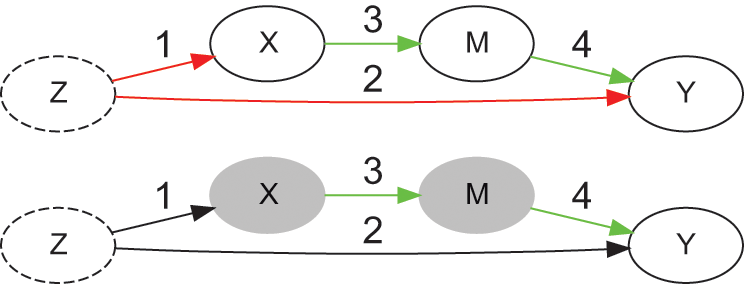
Figure 3 provides an example of a causal graph with a latent variable
 (represented as a dashed oval) that confounds the effect of
 on
on
 . There is a backdoor path between
 and
and
 (colored in red, Y ← Z → X), and a causal path (colored in green, X → M → Y). The first condition of the backdoor criterion is violated (it is not possible to condition on
 ), however
 satisfies the front-door criterion, because
 mediates the only causal path (X → M → Y), the path between
 and
and
 is blocked by collider
 (M → Y ← Z → X), and conditioning on
 blocks the backdoor path between
 and
and
 (Y ← Z → X → M). The adjustment accomplishes that the only remaining association is the one flowing through the causal path.
Example of a causal graph that satisfies the front-door criterion, before (top) and after (bottom) adjustment
4.3.2.4 Instrumental Variables
The front-door adjustment controls for a latent confounder when a mediator exists. In the absence of a mediator, the instrumental variables method allows researchers to control for a latent confounder
 , as long as researchers can find a variable
 that turns
 into a collider, thus blocking the backdoor path through
 .
.
A variable
 satisfies the instrumental variable criterion relative to treatment
 and outcome
 if the following three conditions are true: (i) there is an arrow W → X; (ii) the causal effect of
 on
on
 is fully mediated by
 ; and (iii) there is no backdoor path between
 and
and
 .
.
Intuitively, conditions (i) and (ii) ensure that
 can be used as a proxy for
 , whereas condition (iii) prevents the need for an additional backdoor adjustment to de-confound the effect of
 on
on
 . Figure 4 provides an example of a causal graph with a latent variable
 that confounds the effect of
 on
on
 . There is a backdoor path between
 and
and
 (colored in red, Y ← Z → X), and a causal path (colored in green, X → Y). The first condition of the backdoor criterion is violated (it is not possible to condition on
 ), and the first condition of the front-door criterion is violated (there is no mediator between
 and
and
 ). Variable
 is an instrument, because there is an arrow W → X (arrow number 4),
 mediates the only causal path from
 to
to
 (W → X → Y), and there is no backdoor path between
 and
and
 .
.
Example of a causal graph with an instrumental variable
 , before (top) and after (bottom) adjustment
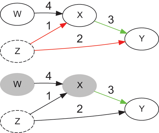
Assuming that Figure 4 represents a linear causal model, the coefficient
 provides a biased estimate of the effect X → Y, due to the confounding effect of
 . To estimate the unconfounded coefficient of effect X → Y, the instrumental variables method estimates first the coefficient of the effect W → X → Y as the slope of the regression line of
 on
on
 ,
,
 , which is the product of coefficients of effects (3) and (4) in Figure 4. The coefficient of effect (4) can be estimated from the slope of the regression line of
 on
on
 ,
,
 . Finally, the adjusted (unconfounded) coefficient of effect X → Y can be estimated as
 . For further reading, see Reference Hernán and RobinsHernán and Robins (2020, chapter 16).
5 Causality in Econometrics
Reference Chen and PearlChen and Pearl (2013) reviewed six of the most popular textbooks in econometrics, concluding that they “deviate significantly from modern standards of causal analysis.” Chen and Pearl find that most textbooks deny the causal content of econometric equations, and confuse causation with association. This section discusses several ways in which the econometrics literature often misunderstands causality.
5.1 Authors often Mistake Causality for Association
First, consider the joint distribution of
 , and the standard econometric model,
 . Second, consider an alternative model with specification,
 . If regression parameters are characteristics of the joint distribution of
 , it should be possible to recover one set of estimates from the other, namely
 ,
,
 , and
, and
 , because associational relations are nondirectional. However, least-squares estimators do not have this property. The parameter estimates from one specification are inconsistent with the parameter estimates from the alternative specification, hence a least-squares model cannot be “just” a statement on the joint distribution
 . If a least-squares model does not model association, what does it model? The answer comes from the definition of the error term, which implies a directed flow of information. In the first specification,
 represents the portion of the outcome
 that cannot be attributed to
 . This unexplained outcome is different from
 , which is the portion of the outcome
 that cannot be attributed to
 . A researcher that chooses the first specification has in mind a controlled experiment where
 causes
 , and he estimates the effect coefficient
 under the least-squares assumption that
 , rather than
 . A researcher that chooses the second specification has in mind a controlled experiment where
 causes
 , and he estimates the effect coefficient
 under the assumption that
 , rather than
 . The vast majority of econometric models rely on least-squares estimators, hence implying causal relationships, not associational relationships (Reference WooldridgeImbens and Wooldridge 2009; Reference Abadie and CattaneoAbadie and Cattaneo 2018).
By choosing a particular model specification and estimating its parameters through least-squares, econometricians inject extra-statistical information consistent with some causal graph. Alternatively, econometricians could have used a Deming (or orthogonal) regression, a type of errors-in-variables model that attributes errors to both
 and
and
 . Figure 5 illustrates the regression lines of: (1) a least-squares model where
 causes
 ; (2) a least-squares model where
 causes
 ; and (3) a Deming regression. Only result (3) characterizes the joint distribution
 , without injecting extra-statistical information.
Three regression lines on the same dataset
The realization that econometric equations model causal relationships may come as a surprise to many economics students and professionals. This surprise is understandable, because econometrics textbooks rarely mention causality, causal discovery, causal graphs, causal mechanisms, or causal inference. Economists are not trained in the estimation of Bayesian networks, design of experiments, or applications of do-calculus.Footnote 23 They are not taught that the causal graph determines the model’s specification, not the other way around, hence the identification of a causal graph should always precede any choice of model specification. Instead, they have been taught debunked specification-searching procedures, such as the stepwise algorithm (an instance of selection bias under multiple testing, see Reference Romano and WolfRomano and Wolf 2005), the general-to-simple algorithm (see Reference GreeneGreene 2012, pp. 178–182), or model selection through trial and error, see Reference ChatfieldChatfield (1995). Section 6.4.2.3 expands on this point, in the context of factor investing.
5.2 Authors often Misunderstand the Meaning of


The least-squares method estimates
 in the equation
 asFootnote 24
 (10)
(10)
For the estimate to be unbiased (
 ), it must occur that
 . This is known as the exogeneity condition. There are two approaches for achieving exogeneity. The first approach, called implicit exogeneity, is to define the error term as
 , thus
 . Under this approach,
 , and
, and
 has merely a distributional (associational) interpretation, as the slope of a regression line. This is the approach adopted by most econometrics textbooks, see for example Reference GreeneGreene (2012), Reference Hill, Griffiths and LimHill et al. (2011), Reference KennedyKennedy (2008), Reference RuudRuud (2000), and Reference WooldridgeWooldridge (2009). A first flaw of this approach is that it cannot answer interventional questions, hence it is rarely useful for building theories. A second flaw is that it is inconsistent with the causal meaning of the least-squares model specification (Section 5.1).
The second approach, called explicit exogeneity, is to assume that
 represents all causes of
 that are uncorrelated to
 . In this case, exogeneity is supported by a causal argument, not by an associational definition. When
 has been randomly assigned, as in an RCT or a natural experiment, exogeneity is a consequence of experimental design. However, in purely observational studies, the validity of this assumption is contingent on the model being correctly specified. Under this second approach,
 , and
, and
 has a causal interpretation, as the expected value of
 given an intervention that sets the value of
 . More formally,
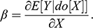 (11)
(11)
Defending the assumption of correct model specification requires the identification of a causal graph consistent with the observed sample. Absent this information,
 loses its causal meaning, and reverts to the simpler associational interpretation that is inadequate for building theories and inconsistent with least-squares’ causal meaning.
The ceteris paribus assumption, so popular among economists, is consistent with the causal interpretation of the estimated
 , whereby the model simulates a controlled experiment. Haavelmo (1944) was among the first to argue that most economists imply a causal meaning when they use their estimated
 . Almost 80 years later, most econometrics textbooks continue to teach an associational meaning of the estimated
 that contradicts economists’ interpretation and use. Accordingly, economists are taught to estimate
 as if it were an associational concept, without regard for causal discovery or do-calculus, while at the same time they interpret and use the estimated
 as if it were a causal concept, leading to spurious claims.
5.3 Authors Often Mistake Association for Causality
Section 5.1 explained how economists often mean causation when they write about association. Oddly, economists also often mean association when they write about causation. A case in point is the so-called Granger causality. Consider two stationary random variables
 and
and
 . Reference GrangerGranger (1969, Reference Granger1980) proposed an econometric test for (linear) causality, based on the equation:
 (12)
(12)
According to Granger,
 causes
 if and only if at least one of the estimated coefficients in
 is statistically significant. This approach was later expanded to multivariate systems, in the form of a vector autoregression specification, see Reference HamiltonHamilton (1994, section 11.2).
The term Granger causality is an unfortunate misnomer. The confusion stems from Granger’s attempt to define causality in terms of sequential association (a characteristic of the joint distribution of probability), see Reference DieboldDiebold (2007, pp. 230–231). However, sequentiality is a necessary, non-sufficient condition for causality (Section 2). Sequential association cannot establish causality, as the latter requires an interventional or natural experiment (Sections 4.1 and 4.2), and in the absence of these, a simulated intervention justified by a discovered or hypothesized causal graph (Section 4.3). For example, a Granger causality test will conclude that a rooster’s crow (
 ) causes the sun to dawn (
 ), because
 is statistically significant after controlling for lags of
 . And yet, it is trivial to falsify the claim that a rooster’s crow is a cause of dawn, by silencing the rooster before dawn, or by forcing it to crow at midnight (an intervention). A second problem with Granger causality is that, if both
 and
and
 are caused by
 (a confounder), Granger’s test will still falsely conclude that
 causes
 (see Figure 1). Granger causality is misleading in a causally insufficient multivariate time series (Peters et al. Reference Peters, Janzing and Scholkopf2017, pp. 205–208). A third problem is that the test itself is susceptible to selection bias, because the selection of lagged variables involves multiple testing across a large number of potential specifications that are not informed by a causal graph, for example through stepwise specification-searching algorithms. A fourth problem is that it assumes that the causal relation must be linear.
Reference GrangerGranger (1969) remains one of the most-cited articles in the econometrics literature, with over 33,000 citations, and it has become Granger’s second most-cited article. As Figure 6 illustrates, that publication receives thousands of new citations each year, and that number keeps rising, with 2,294 publications referencing it in the year 2021 alone. This confusion of association for causality has led to numerous misinformed claims in the factor investing literature (see Reference Schuller, Haberl and ZaichenkovSchuller et al. 2021 for a survey of claims based on Granger causality). While Granger causality may be used as a simple tool to help decide the direction of causal flow between two unconfounded variables (rather than the existence of causal flow), the field of causal discovery has developed more sophisticated methods to that purpose (see Reference Peters, Janzing and ScholkopfPeters et al. 2017, chapter 4).
Citations of Reference GrangerGranger (1969).
I cannot end this section without recognizing a few remarkable economists who, defying the resistance from their peers, have fought to bring the rigor of causal inference into their field of study. Section 4.3.2.4 already discussed the method of instrumental variables, first proposed in 1928 by economist P. G. Wright. Section 5.2 mentioned Haavelmo’s 1944 paper on the meaning of
 , whose insights continue to be ignored today to a large extent (Reference PearlPearl 2015). The original idea of the DID approach first appeared in labor economics, see Reference Ashenfelter and CardAshenfelter and Card (1986). In the year 2021, Joshua Angrist and Guido Imbens received (in conjunction with David Card) the Nobel Memorial Prize in Economics in recognition “for their methodological contributions to the analysis of causal relationships” in the context of natural experiments (see Section 4.2). Several authors have recently applied the RDD approach to corporate finance, such as Reference Bronzoni and IachiniBronzoni and Iachini (2014), Reference FlammerFlammer (2015), and Reference Malenko and ShenMalenko and Shen (2016). Reference Angrist and PischkeAngrist and Pischke (2010) have called for a “credibility revolution,” urging fellow economists to improve the reliability of their empirical work through the design of interventional studies and natural experiments. These academics offer a rare but inspiring example that ought to be emulated throughout the entire field of economics. On the other hand, asset pricing remains to this day staunchly oblivious to rigorous causal reasoning. Paraphrasing Reference LeamerLeamer (1983), factor researchers have not yet taken the “con” out of econometrics, with the dire consequences described in the following section.
6 Causality in Factor Investing
The previous section outlined the prevailing state of confusion between association and causation in the field of econometrics. This section focuses on how financial economists have often (mis)applied econometrics to factor investing, leading to a discipline based on shaky foundations and plagued with false discoveries (Reference HarveyHarvey 2017).
Factor investing can be defined as the investment approach that targets the exposure to measurable characteristics (called “factors”) that presumably explain differences in the performance of a set of securities.Footnote 26 This is an evolution of the Asset Pricing Theory literature,Footnote 27 inspired by the seminal work of Reference Schipper and ThompsonSchipper and Thompson (1981), that uses factor analysis and principal component analysis to validate those characteristics (Reference FersonFerson 2019, p. 130). For example, proponents of the value factor believe that a portfolio composed of stocks with a high book-to-market equity (called “value stocks”) will outperform a portfolio composed of stocks with a low book-to-market equity (called “growth stocks”). In search of supportive empirical evidence, factor researchers generally follow one of two procedures. In the first procedure, inspired by Reference Fama and MacBethFama and MacBeth (1973), a researcher gathers returns of securities (
 ), explanatory factors (
 ), and control variables (
 ). The researcher then estimates through least-squares the parameters (also called factor exposures or factor loadings) of a cross-sectional regression model with general form
 for each time period, and computes the mean and standard deviation of those parameter estimates across all periods (Reference CochraneCochrane 2005, pp. 245–251). In the second procedure, inspired by Reference Fama and FrenchFama and French (1993), a researcher ranks securities in an investment universe according to a characteristic, and carries out two parallel operations on that ranking: (a) partition the investment universe into subsets delimited by quantiles, and compute the time series of average returns for each subset; and (b) compute the returns time series of a long-short portfolio, where top-ranked securities receive a positive weight and bottom-ranked securities receive a negative weight. A researcher interested in a multifactor analysis will apply operations (a) and (b) once for each factor (for operation (a), this means further partitioning each subset). For each subset, the researcher then estimates through least-squares the parameters of a time-series regression model with general form
 , where
 represents one time series computed in (a),
 represents the (possibly several) time series computed in (b), and
 represents the times series of control variables chosen by the researcher.
The goal of both procedures is not to explain changes in average returns over time (a time-series analysis), but rather to explain differences in average returns across securities. The first procedure accomplishes this goal through averaging cross-sectional regressions coefficients computed on explanatory factors. The second procedure accomplishes this goal through a regression of quantile-averaged stock returns against the returns attributed to neutralized factors. Following the econometric canon, researchers state their case by showing that the estimated value of
 is statistically significant, with the interpretation that investors holding securities with exposure to factor
 are rewarded beyond the reward received from exposure to factors in
 .
.
6.1 Causal Content
Factor researchers almost never state explicitly the causal assumptions that they had in mind when they made various modeling decisions, and yet those assumptions shape their analysis. A different set of causal assumptions would have led to different data pre-processing, choice of variables, model specification, choice of estimator, choice of tested hypotheses, interpretation of results, portfolio design, etc. Some of these causal assumptions are suggested by the data, and some are entirely extra-statistical. I denote causal content the set of causal assumptions, whether declared or undeclared, that are embedded in a factor model’s specification, estimation, interpretation, and use. Factor investing strategies reveal part of their causal content in at least four ways.
First, the causal structure assumed by the researcher determines the model specification. A factor investing strategy is built on the claim that exposure to a particular factor (
 ) causes positive average returns above the market’s (
 ), and that this causal effect (X → Y, a single link in the causal graph) is strong enough to be independently monetizable through a portfolio exposed to
 . A researcher only interested in modelling the joint distribution
 would surely use more powerful techniques from the machine learning toolbox than a least-squares estimator, such as nonparametric regression methods (e.g., random forest regression, support-vector regression, kernel regression, or regression splines). Factor researchers’ choice of least-squares, explanatory variables, and conditioning variables, is consistent with the causal structure that they wish to impose (Section 5.1).Footnote 28
Second, the estimation of
 prioritizes causal interpretation over predictive power. If factor researchers prioritized predictive power, they would: (a) use estimators with lower mean-square error than least-squares, by accepting some bias in exchange for lower variance (Reference Mullainathan and SpiessMullainathan and Spiess 2017; Reference Athey and ImbensAthey and Imbens 2019). Examples of such estimators include ridge regression, LASSO, and elastic nets; or (b) use as loss function a measure of performance, such as the Sharpe ratio (for a recent example, see Reference Cong, Tang, Wang and ZhangCong et al. 2021). So not only researchers believe that
 is a function of
 (a causal concept), but they are also willing to sacrifice as much predictive power (an associational concept) as necessary to remove all bias from
 . The implication is that factor researchers assume that the errors are exogenous causes of
 , uncorrelated to
 (the explicit exogeneity assumption). Factor researchers’ choice of least-squares is consistent with their interpretation of the estimated
 as a causal effect (Section 5.2).
Third, factor researchers place strong emphasis on testing the null hypothesis of
 (no causal effect) against the alternative
 (causal effect), and expressing their findings through p-values. In contrast, machine-learners are rarely interested in estimating individual p-values, because they assess the importance of a variable in predictive (associational) terms, with the help of associational concepts such as mean-decrease accuracy (MDA), mean-decrease impurity (MDI), and Shapley values (Reference López de PradoLópez de Prado 2018). Factor researchers’ use of p-values is consistent with the claim of a significant causal effect.Footnote 29
Fourth, factor investors build portfolios that overweight stocks with a high exposure to
 and underweight stocks with a low exposure to
 , at the tune of one separate portfolio for each factor. A factor investor may combine those separate factor portfolios into an aggregate multifactor portfolio, however the reason behind that action is diversification, not monetizing a multifactor prediction. This approach to building portfolios stands in contrast with how other investors use predictions to form portfolios. Investors who rely on predictive models build portfolios exposed to the residual (
 ) rather than portfolios exposed to a particular factor (
 ), hence for them biased estimates of
 are not a concern. Factor researchers’ approach to portfolio design is consistent with the monetization of a causal claim rather than a predictive (associational) claim.
In conclusion, the objective of a factor model such as
 is not to predict
 conditioned on
 and
and
 (
(
 ), but to estimate the causal effect of
 on
on

 , which can be simulated on the observed sample by controlling for confounder
 . The implication is that researchers use factors as if they had assumed explicit exogeneity, and their chosen model specification
 is consistent with a particular causal graph (see Section 5.2), of which Figure 7 is just one possibility among several. It is the responsibility of the researcher to declare and justify what particular causal graph informed the chosen specification, such that the exogeneity assumption holds true.
Causal graph for which the specification
 estimates the causal effect of
 on
on
 , while adjusting for the confounding effect of

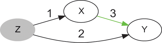
6.2 Omitted Mediation Analysis
Several papers have proposed alternative explanations for various factors, which can be grouped into two broad themes: (a) investment-based explanations; and (b) production-based explanations. For example, Reference Fama and FrenchFama and French (1996) argue that stocks approaching bankruptcy experience a price correction, which in turn is reflected as high value (a high book-to-market ratio). According to this explanation, investors holding portfolios of high-value stocks demand a premium for accepting a non-diversifiable risk of bankruptcy. Reference Berk, Green and NaikBerk et al. (1999) argue that, should firms’ assets and growth options change in predictable ways, that would impart predictability to changes in a firm’s systematic risk and its expected return. Reference JohnsonJohnson (2002) explains that the momentum effect in stock returns does not necessarily imply investor irrationality, heterogeneous information, or market frictions, because simulated efficient markets for stocks exhibit price momentum when expected dividend growth rates vary over time. Reference Gomes, Kogan and ZhangGomes et al. (2003) simulate a dynamic general equilibrium economy, concluding that the size and value factors can be consistent with a single-factor conditional CAPM. Reference ZhangZhang (2005) simulates an economy that exhibits many empirical irregularities in the cross-section of returns. Reference Sagi and SeasholesSagi and Seasholes (2007) claim that backtested performance of momentum strategies is particularly good for firms with high revenue growth, low costs, or valuable growth options. Reference Liu, Whited and ZhangLiu et al. (2009), Reference Li, Livdan and ZhangLi et al. (2009), and Reference Li and ZhangLi and Zhang (2010) associate market anomalies with corporate investment levels, using Tobin’s q-ratio (the ratio between a physical asset’s market value and its replacement value). Reference Liu and ZhangLiu and Zhang (2008) study the association between momentum portfolio returns and shifts in factor loadings on the growth rate of industrial production, concluding that the growth rate of industrial production is a priced risk factor. See Reference CochraneCochrane (2005, pp. 442–453) for additional explanations of factors, some of which are highly speculative or mutually contradictory.
These explanations, in the form of plausible economic rationales, do not rise to the level of scientific theories, for three primary reasons outlined in Sections 3 and 4. First, the authors of these explanations have not declared the causal relationship hypothetically responsible for the observed phenomenon. Second, the authors have not elucidated the ideal interventional study that would capture the causal effect of interest. A Gedankenexperiment, even if unfeasible, has the benefit of communicating clearly the essence of the causal relationship, and the counterfactual implications under various scenarios. Third, when the ideal interventional study is unfeasible, the authors have not proposed a method to estimate the causal effect through observational data (a natural experiment, or a simulated intervention). Consequently, while these economic rationales are plausible, they are also experimentally unfalsifiable. Following Pauli’s criterion, the explanations proposed by factor investing researchers are “not even wrong” (Reference LiptonLipton 2016). As discussed in Section 3, scientific knowledge is built on falsifiable theories that describe the precise causal mechanism by which
 causes
 . Value investors may truly receive a reward (
 ) for accepting an undiversifiable risk of bankruptcy (
 ), but how precisely does this happen, and why is book-to-market the best proxy for bankruptcy risk? Despite of factor models’ causal content, factor researchers rarely declare the causal mechanism by which
 causes
 . Factor papers do not explain precisely how a firm’s (or collection of firms’) exposure to a factor triggers a sequence of events that ends up impacting stock average returns; nor do those papers derive a causal structure from the observed data; nor do those papers analyze the causal structure (forks, chains, immoralities); nor do those papers make an effort to explain the role played by the declared variables (treatment, confounder, mediator, collider, etc.); nor do those papers justify their chosen model specification in terms of the identified causal structure (an instance of concealed assumptions).
6.2.1 Example of Factor Causal Mechanism
For illustrative purposes only, and without a claim of accuracy, consider the following hypothetical situation. A researcher observes the tendency of prices (
 ) to converge toward the value implied by fundamentals (
 ). The researcher hypothesizes that large divergences between prices and fundamental values (HML) trigger the following mechanism: (1) As investors observe HML, they place bets that the divergence will narrow, which cause orderflow imbalance (OI); (2) the persistent OI causes permanent market impact, which over some time period (
 ) pushes prices toward fundamental values (PC, for price convergence).Footnote 30 An investment strategy could be proposed, whereby a fund manager acts upon (1) before (2) takes place.
As stocks rally, investors are more willing to buy them, making some of them more expensive relative to fundamentals, and as stocks sell off, investors are less willing to buy them, making some of them cheaper relative to fundamentals. The researcher realizes that the
 mechanism is disrupted by diverging price momentum (MOM), that is, the momentum that moves prices further away from fundamentals, thus contributing to further increases of HML. The researcher decides to add this information to the causal mechanism as follows: (3) high MOM affects future prices in a way that delays PC; and (4) aware of that delay, investors are wary of acting upon HML in the presence of high MOM (i.e., placing a price-convergence bet too early). Accordingly, MOM is a likely confounder, and the researcher must block that backdoor path
 . Fortunately, MOM is observable, thus eligible for backdoor adjustment (Section 4.3.2.2). But even if MOM were not observable, a front-door adjustment would be possible, thanks to the mediator OI (Section 4.3.2.3).
The above description is consistent with the following system of structural equations:
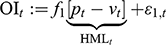 (13)
(13)
 (14)
(14)
 (15)
(15)
where
 are the functions associated with each causal effect (the arrows in a causal graph), and
 are exogenous unspecified causes. The symbol “
 ” indicates that the relationship is causal rather than associational, thus asymmetric (e.g., the right-hand side influences the left-hand side, and not the other way around). The researcher applies causal discovery tools on a representative dataset, and finds that the derived causal structure is compatible with his theorized data-generating process. Using the discovered causal graph, he estimates the effect of HML on OI, and the effect of OI on PC, with a backdoor adjustment for MOM. The empirical analysis suggests that HML causes PC, and that the effect is mediated by OI. Encouraged by these results, the researcher submits an article to a prestigious academic journal.
Upon review of the researcher’s journal submission, a referee asks why the model does not control for bid-ask spread (BAS) and market liquidity factors (LIQ). The referee argues that OI is not directly observable, and its estimation may be biased by passive traders. For instance, a large fund may decide to place passive orders at the bid for weeks, rather than lift the offers, in order to conceal their buying intentions. Those trades will be labeled as sale-initiated by the exchange, even though the persistent OI comes from the passive buyer (a problem discussed in Reference Easley, de Prado and O’HaraEasley et al. 2016). The referee argues that BAS is more directly observable, and perhaps a better proxy for the presence of informed traders. The researcher counter-argues that he agrees that (5) OI causes market makers to widen BAS, however (6) PC also forces market makers to realize losses, as prices trend, and market makers’ reaction to those losses is also the widening of BAS. Two consequences of BAS widening are (7) lower liquidity provision and (8) greater volatility. Accordingly, BAS is a collider, and controlling for it would open the noncausal path of association
 (see Section 6.4.2.2). While the referee is not convinced with the relevance of (6), he is satisfied that the researcher has clearly stated his assumptions through a causal graph. Readers may disagree with the stated assumptions, which the causal graph makes explicit, however, under the proposed causal graph everyone agrees that controlling for either BAS or LIQ or VOL would be a mistake.
The final causal path and causal graph are reflected in Figure 8. By providing this causal graph and mechanism, the researcher has opened himself to falsification. Referees and readers may propose experiments designed to challenge every link in the causal graph. For example, researchers can test link (1) through a natural experiment, by taking advantage that fundamental data is updated at random time differences between stocks. The treatment effect for link (1) may be estimated as the difference in OI over a given period between stocks where HML has been updated versus stocks where HML has not been updated yet. Links (2), (5), (6), (7), and (8) may be tested through controlled and natural experiments similar to those mentioned in Section 3.3. Link (3) is a mathematical statement that requires no empirical testing. To test link (4), a researcher may split stocks with similar HML into two groups (a cohort study, see Section 4.2): the first group is composed of stocks where MOM is increasing HML, and the second group is composed of stocks where MOM is reducing HML. Since the split is not random, the researcher must verify that the two groups are comparable in all respects other than MOM’s direction. The treatment effect may be measured as the two groups’ difference in: (a) sentiment extracted from text, such as analyst reports, financial news, social media (see Reference Das and ChenDas and Chen 2007; Reference Baker and WurglerBaker and Wurgler 2007); (b) sentiment from surveys; or (c) exposures reports in SEC 13F forms. If link (4) is true, MOM dampens investors’ appetite for HML’s contrarian bets, which is reflected in the groups’ difference.
Example of a hypothesized causal mechanism of HML (in the box) within a hypothesized causal graph
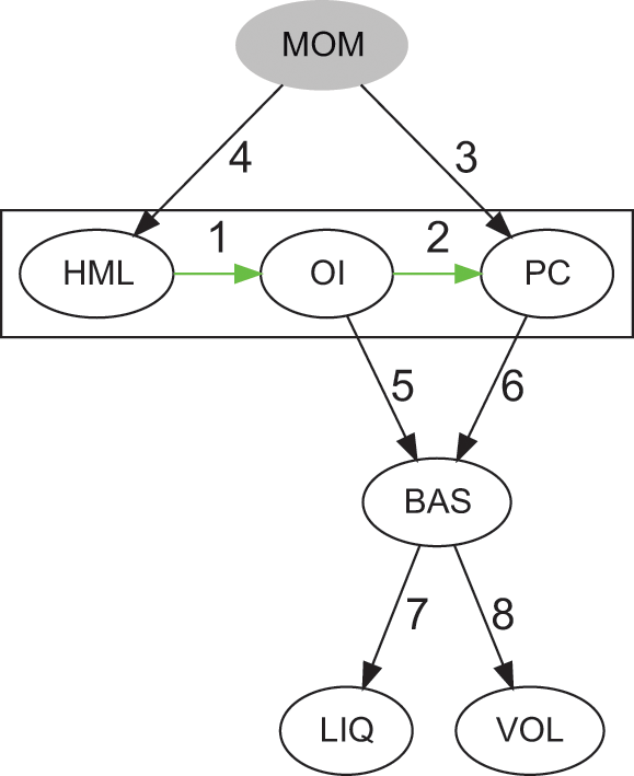
These experiments are by no means unique, and many alternatives exist. The opportunities for debunking this theory will only grow as more alternative datasets become available. Contrast this openness with the narrow opportunities offered by factor investing articles currently published in journals, which are essentially limited to: (a) in-sample replication of a backtest, and (b) structural break analyses for in-sample versus out-of-sample performance.
6.3 Causal Denial
Associational investment strategies do not have causal content. Examples include statistical arbitrage (Reference Rad, Low and FaffRad et al. 2016), sentiment analysis (Reference Katayama and TsudaKatayama and Tsuda 2020), or alpha capture (Reference IsichenkoIsichenko 2021, pp. 129–154). Authors of associational investment strategies state their claims in terms of distributional properties, for example, stationarity, ergodicity, normality, homoscedasticity, serial independence, and linearity. The presence of causal content sets factor investing strategies apart, because these investment strategies make causal claims. A causal claim implies knowledge of the data-generating process responsible, among other attributes, for all distributional properties claimed by associational studies. Causal claims therefore require stronger empirical evidence and level of disclosure than mere associational claims. In the context of investment strategies, this translates among other disclosures into: (i) making all causal assumptions explicit through a causal graph; (ii) stating the falsifiable causal mechanism responsible for a claimed causal effect; and (iii) providing empirical evidence in support of (i) and (ii).
Should factor researchers declare causal graphs and causal mechanisms, they would enjoy two benefits essential to scientific discovery. First, causal graphs like the one displayed in Figure 8 would allow researchers to make their causal assumptions explicit, communicate clearly the role played by each variable in the hypothesized phenomenon, and apply do-calculus rules for debiasing estimates. This information is indispensable for justifying the proposed model specification. Second, stating the causal mechanism would provide an opportunity for falsifying a factor theory without resorting to backtests. Even if a researcher p-hacked the factor model, the research community would still be able to design creative experiments aimed at testing independently the implications of every link in the theorized causal path, employing alternative datasets. Peer-reviewers’ work would not be reduced to mechanical attempts at reproducing the author’s calculations.
The omission of causal graphs and causal mechanisms highlights the logical inconsistency at the heart of the factor investing literature: on one hand, researchers inject causal content into their models, and use those models in a way consistent with a causal interpretation (Section 6.1). On the other hand, researchers almost never state a causal graph or falsifiable causal mechanism, in denial or ignorance of the causal content of factor models, hence depriving the scientific community of the opportunity to design experiments that challenge the underlying theory and assumptions (Section 6.2). Under the current state of causal confusion, researchers report the estimated
 devoid of its causal meaning (the effect on
 of an intervention on
 ), and present p-values as if they merely conveyed the strength of associations of unknown origin (causal and noncausal combined).
The practical implication of this logical inconsistency is that the factor investing literature remains at a phenomenological stage, where spurious claims of investment factors are accepted without challenge. Put simply: without a causal mechanism, there is no investment theory; without investment theory, there is no falsification; without falsification, investing cannot be scientific.
This does not mean that investment factors do not exist; however, it means that the empirical evidence presented by factor researchers is insufficient and flawed by scientific standards. Causal denial (or ignorance) is a likely reason for the proliferation of spurious claims in the factor investing studies, and the poor performance delivered by the factor-based investment funds, for the reasons explained next.
6.4 Spurious Investment Factors
The out-of-sample performance of factor investing has been disappointing. One of the broadest factor investing indices is the Bloomberg–Goldman Sachs Asset Management US Equity Multi-Factor Index (BBG code: BGSUSEMF <Index>). It tracks the long/short performance of the momentum, value, quality, and low-risk factors in US stocks (Bloomberg 2021). Its annualized Sharpe ratio from May 2, 2007 (the inception date) to December 2, 2022 (this Element’s submission date) has been 0.29 (t-stat = 1.16, p-value = 0.12), and the average annualized return has been 1.13 percent. This performance does not include: (a) transaction costs; (b) market impact of order execution; (c) cost of borrowing stocks for shorting positions; (d) management and incentive fees. Also, this performance assigns a favorable 0 percent risk-free rate when computing the excess returns. Using the 6-month US Government bond rates (BBG code: USGG6M <Index>) as the risk-free rates, the Sharpe ratio turns negative. Figure 9 plots the performance of this broad factor index from inception, without charging for the above costs (a)–(d). After more than fifteen years of out-of-sample performance, factor investing’s Sharpe ratio is statistically insignificant at any reasonable rejection threshold.
Performance of the Bloomberg – Goldman Sachs Asset Management US Equity Multi-Factor Index, since index inception (base 100 on May 2, 2007)
It takes over 31 years of daily observations for an investment strategy with an annualized Sharpe ratio of 0.29 to become statistically significant at a 95 percent confidence level (see Bailey and Reference Bailey and López de PradoLópez de Prado (2012) for details of this calculation). If the present Sharpe ratio does not decay (e.g., due to overcrowding, or hedge funds preempting factor portfolio rebalances), researchers will have to wait until the year 2039 to reject the null hypothesis that factor investing is unprofitable, and even then, they will be earning a gross annual return of 1.13 percent before paying for costs (a)–(d).
There is a profound disconnect between the unwavering conviction expressed by academic authors and the underwhelming performance experienced by factor investors. A root cause of this disconnect is that factor investing studies usually make spurious claims, of two distinct types.
6.4.1 Type-A Spuriosity
I define an empirical claim to be of type-A spurious when a researcher mistakes random variability (noise) for signal, resulting in a false association. Selection bias under multiple testing is a leading cause for type-A spuriosity. Type-A spuriosity has several distinct attributes: (a) it results in type-1 errors (false positives); (b) for the same number of trials, it has a lower probability to take place as the sample size grows (Reference López de PradoLópez de Prado 2022b); and (c) it can be corrected through multiple-testing adjustments, such as Reference HochbergHochberg (1988) or Bailey and Reference LópezLópez de Prado (2014).
In the absence of serial correlation, the expected return of a type-A spurious investment factor is zero, before transaction costs and fees (Reference Bailey and López de PradoBailey et al. 2014). Next, I discuss the two main reasons for type-A spuriosity in the factor investing literature.
6.4.1.1 P-Hacking
The procedures inspired by Reference Fama and MacBethFama and MacBeth (1973) and Reference Fama and FrenchFama and French (1993) involve a large number of subjective decisions, such as fit window length, fit frequency, number of quantiles, definition of long-short portfolios, choice of controls, choice of factors, choice of investment universe, data cleaning and outlier removal decisions, start and end dates, etc. There are millions of potential combinations to pick from, many of which could be defended on logical grounds. Factor researchers routinely run multiple regressions before selecting a model with p-values below their null-rejection threshold. Authors report those minimal p-values without adjusting for selection bias under multiple testing, a malpractice known as p-hacking. The problem is compounded by publication bias, whereby journals accept papers without accounting for: (a) the number of previously rejected papers; and (b) the number of previously accepted papers. Reference Harvey, Liu and ZhuHarvey et al. (2016) conclude that “most claimed research findings in financial economics are likely false.” The consequence is, factor investments do not perform as expected, and results are not replicated out-of-sample.
Other fields of research have addressed p-hacking decades ago. Statisticians have developed methods to determine the familywise error rate (Reference HochbergHochberg 1988; Reference WhiteWhite 2000; Reference Romano and WolfRomano and Wolf 2005) and false discovery rate (Reference Benjamini and HochbergBenjamini and Hochberg 1995).Footnote 31 Medical journals routinely demand the logging, reporting, and adjustment of results from all trials. Since 2008, laboratories are required by U.S. law to publish the results from all trials within a year of completion of a clinical study (Section 801 of the Food and Drug Administration Amendments Act of 2007).
While most disciplines are taking action to tackle the replication crisis, the majority of members of the factor investing research community remain unwaveringly committed to p-hacking. There are two possible explanations for their choice: ignorance and malpractice. Factor researchers have not been trained to control for multiple testing. To this day, all major econometrics textbooks fail to discuss solutions to the problem of conducting inference when more than one trial has taken place. As Reference HarveyHarvey (2017, p. 1402) lamented, “our standard testing methods are often ill equipped to answer the questions that we pose. Other fields have thought deeply about testing” (emphasis added). However, ignorance alone does not explain why some factor investing authors argue that multiple testing is not a problem, against the advice of mathematical societies (Reference Wasserstein and LazarWasserstein and Lazar 2016). Reference HarveyHarvey (2022) explains the stance of p-hacking deniers by pointing at the commercial interests that control financial academia.
6.4.1.2 Backtest Overfitting
A backtest is commonly defined as a historical simulation of how a systematic strategy would have performed in the past (Reference López de PradoLópez de Prado 2018, chapter 11). Factor researchers often present backtests as evidence that a claimed causal effect is real. However, a backtest is neither a controlled experiment, nor an RCT, nor a natural experiment, because it does not allow the researcher to intervene on the data-generating process (a do-operation), and a simulation does not involve the researcher’s or Nature’s random assignment of units to groups. Accordingly, a backtest has no power to prove or disprove a causal mechanism. At best, a backtest informs investors of the economic potential of an investment strategy, under the assumption that history repeats itself (a distributional inductive belief, hence associational and noncausal).
Factor researchers rarely report or adjust for the number of trials involved in a backtest (Fabozzi and Reference López de PradoLópez de Prado 2018; Reference López de Prado and LewisLópez de Prado and Lewis 2019; Reference López de PradoLópez de Prado 2019). As demonstrated by the False Strategy Theorem, it is trivial to overfit a backtest through selection bias under multiple testing, making it hard to separate signal from noise (Reference Bailey and López de PradoBailey et al. 2014; Reference LópezBailey and López de Prado 2014, Reference Bailey and López de Prado2021).
The outcome from a backtest is yet another associational claim. Replicating that associational claim does not prove that the association is causal, or that the noncausal association is true. Two researchers can independently mistake the same noise for signal, particularly when they narrow their modeling choices to linear regressions with similar biases. Obtaining similar backtest results on different sets of securities (e.g., from a different sector, or geography, or time period) does not constitute causal evidence, as those findings can be explained in terms of the same noncausal association being present on the chosen sets, or in terms of a statistical fluke.
6.4.2 Type-B Spuriosity
An association is true if it is not type-A spurious, however that does not mean that the association is causal. I define an empirical claim to be type-B spurious when a researcher mistakes association for causation. A leading cause for type-B spuriosity is systematic biases due to misspecification errors. A model is misspecified when its functional form is incongruent with the functional form of the data-generating process, and the role played by the variables involved. Type-B spuriosity has several distinct attributes: (a) it results in type-1 errors and type-2 errors (false positives and false negatives); (b) it can occur with a single trial; (c) it has a greater probability to take place as the sample size grows, because the noncausal association can be estimated with lower error; and (d) it cannot be corrected through multiple-testing adjustments. Its correction requires the injection of extra-statistical information, in the form of a causal theory.
The expected return of a type-B spurious investment factor is misattributed, as a result of the biased estimates. Also, type-B spurious investment factors can exhibit time-varying risk premia (more on this in Section 6.4.2.1).
Type-A and type-B spuriosity are mutually exclusive. For type-B spuriosity to take place, the association must be noncausal but true, which precludes that association from being type-A spurious. While type-A spuriosity has been studied with some depth in the factor investing literature, relatively little has been written about type-B spuriosity. Next, I discuss the main reasons for type-B spuriosity in factor investing.
6.4.2.1 Under-Controlling
Consider a data-generating process where one of its equations is
 , such that
 and
and
 is white noise. The process is unknown to a researcher, who attempts to estimate the causal effect of
 on
on
 by fitting the equation
 on a sample
 produced by the process. This incorrect specification choice makes
 , and
, and
 . However, if
 is correlated with
 ,
,
 , hence
 . This is a problem, because the least-squares method assumes
 (the exogeneity assumption, see Section 5.2). Missing one or several relevant variables biases the estimate of
 , potentially leading to spurious claims of causality. A false positive occurs when
 for
for
 , and a false negative occurs when
 for
for
 .
.
Econometrics textbooks do not distinguish between types of missing variables (see, for example, Reference GreeneGreene 2012, section 4.3.2), yet not all missing variables are created equal. There are two distinct cases that researchers must consider. In the first case, the second equation of the data-generating process is
 , where
 and
and
 is white noise. In this case,
 is a mediator (
 causes
 , and
, and
 causes
 ), and the chosen specification biases the estimation of the direct effect
 ; however,
 can still be interpreted as a total causal effect (through two causal paths with the same origin and end). The causal graph for this first case is displayed at the top of Figure 10. In the second case, the second equation of the data-generating process is
 , where
 and
and
 is white noise. In this case,
 is a confounder (
 causes
 and
and
 ), the chosen specification also biases
 , and
, and
 does not measure a causal effect (whether total or direct).Footnote 32 The causal graph for this second case is displayed at the bottom of Figure 10.
Variable
 as mediator (top) and confounder (bottom)
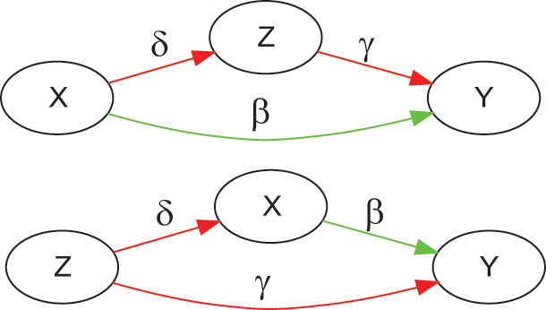
Assuming that the white noise is Gaussian, the expression
 reduces to

 (16)
(16)
where
 is the bias due to the missing confounder. The Appendix contains a proof of the above proposition. The intuition behind
 is that a necessary and sufficient condition for a biased estimate of
 is that
 and
and
 , because when both parameters are nonzero, variable
 is a confounder.
A first consequence of missing a confounder is incorrect performance attribution and risk management. Part of the performance experienced by the investor comes from a misattributed risk characteristic
 , which should have been hedged by a correctly specified model. The investor is exposed to both, causal association (from
 ), as intended by the model’s specification, and noncausal association (from
 ), which is not intended by the model’s specification.
A second consequence of missing a confounder is time-varying risk premia. Consider the case where the market rewards exposure to
 and
and
 (
(
 ,
,
 ). Even if the two risk premia remain constant, changes over time in
 will change
 . In particular, for a sufficiently negative value of
 , then
 . Performance misattribution will mislead investors into believing that the market has turned to punish exposure to risk characteristic
 , when in reality their losses have nothing to do with changes in risk premia. The culprit is a change in the covariance between the intended exposure (
 ) and the unintended exposure that should have been hedged (
 ). Authors explain time-varying risk premia as the result to changes in expected market returns (e.g., Reference EvansEvans 1994; Reference AndersonAnderson 2011; and Reference CochraneCochrane 2011), and asset managers’ marketing departments justify their underperformance in terms of temporary changes in investor or market behavior. While these explanations are plausible, they seem to ignore that time-varying risk premia is consistent with a missing confounder (an arguably more likely and parsimonious, hence preferable, explanation). For example, consider the causal graph in Figure 8, where MOM confounds the estimate of the effect of HML on PC. If an asset manager under-controls for MOM, the value investment strategy will be exposed to changes in the covariance between MOM and HML. The asset manager may tell investors that the value strategy is losing money because of a change in value’s risk premium, when the correct explanation is that the product is defective, as a result of under-controlling. Changes in the covariance between MOM and HML have nothing to do with value’s or momentum’s true risk premia, which remain unchanged (like the direct causal effects,
 and
and
 ). This flaw of type-B spurious factor investing strategies makes them untrustworthy.
The partial correlations method allows researchers to control for observable confounders when the causal effect is linear and the random variables jointly follow an elliptical (including multivariate normal) distribution, multivariate hypergeometric distribution, multivariate negative hypergeometric distribution, multinomial distribution, or Dirichlet distribution (Reference Baba, Shibata and SibuyaBaba et al. 2004). A researcher is said to “control” for the confounding effect of
 when he adds
 as a regressor in an equation set to model the effect of
 on
on
 . Accordingly, the new model specification for estimating the effect of
 on
on
 is
is
 . This is a particular application of the more general backdoor adjustment (Section 4.3.2.2), and by far the most common confounder bias correction method used in regression analysis. This adjustment method relies on a linear regression, thus inheriting its assumptions and limitations. In particular, the partial correlations method is not robust when the explanatory variables exhibit high correlation (positive or negative) with each other (multicollinearity).
6.4.2.2 Over-Controlling
The previous section explained the negative consequences of under-controlling (e.g., missing a confounder). However, over-controlling is not less pernicious. Statisticians have been trained for decades to control for any variable
 associated with
 that is not
 (Reference Pearl and MacKenziePearl and MacKenzie 2018, pp. 139, 152, 154, 163), regardless of the role of
 in the causal graph (the so-called omitted variable problem). Econometrics textbooks dismiss as a harmless error the inclusion of an irrelevant variable, regardless of the variable’s role in the causal graph. For example, Reference GreeneGreene (2012, section 4.3.3) states that the only downside to adding superfluous variables is a reduction in the precision of the estimates. This grave misunderstanding has certainly led to countless type-B spurious claims in economics.
In recent years, do-calculus has revealed that some variables should not be controlled for, even if they are associated with
 . Figure 11 shows two examples of causal graphs where controlling for
 will lead to biased estimates of the effect of
 on
on
 .
.
Variable
 as controlled mediator (top) and controlled collider (bottom)
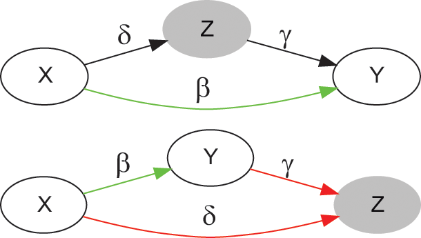
Common examples of over-controlling include controlling for variables that are mediators or colliders relative to the causal path from
 to
to
 .Footnote 33 Controlling for a collider is a mistake, as it opens a backdoor path that biases the effect’s estimation (Berkson’s fallacy, see Reference BerksonBerkson 1946). Controlling for a mediator interferes with the mediated effect (
 ) and the total causal effect (
 plus
plus
 ) that the researcher may wish to assess, leaving only the direct effect
 . In the case of the top causal graph in Figure 11, a researcher could estimate the mediated effect
 as the difference between the total effect (
 plus
plus
 ) and the direct effect (
 ).
).
Over-controlling a collider and under-controlling a confounder have the same impact on the causal graph: allowing the flow of association through a backdoor path (Section 4.3.2.2). Consequently, over-controlled models can suffer from the same conditions as under-controlled models, namely (i) biased estimates, as a result of noncompliance with the exogeneity assumption; and (ii) time-varying risk premia. Black-box investment strategies take over-controlling to the extreme. Over-controlling explains why quantitative funds that deploy black-box investment strategies routinely transition from delivering systematic profits to delivering systematic losses, and there is not much fund managers or investors can do to detect that transition until it is too late.
The only way to determine precisely which variables a researcher must control for, in order to block (or keep blocked) noncausal paths of association, is through the careful analysis of a causal graph (e.g., front-door criterion and backdoor criterion). The problem is, factor researchers almost never estimate or declare the causal graphs associated with the phenomenon under study (Section 6.2). Odds are, factor researchers have severely biased their estimates of
 by controlling for the wrong variables, which in turn has led to false positives and false negatives.
6.4.2.3 Specification-Searching
Specification-searching is the popular practice among factor researchers of choosing a model’s specification (including the selection of variables and functional forms) based on the resulting model’s explanatory power. To cite one example, consider the three-factor model introduced by Reference Fama and FrenchFama and French (1993), and the five-factor model introduced by Reference Fama and FrenchFama and French (2015). Reference Fama and FrenchFama and French (2015)’s argument for adding two factors to their initial model specification was that “the five-factor model performs better than the three-factor model when used to explain average returns.”
These authors’ line of argumentation is self-contradictory. The use of explanatory power (an associational, noncausal concept) for selecting the specification of a predictive model is consistent with the associational goal of that analysis; however, it is at odds with the causal content of a factor model. In the context of factor models, specification-searching commingles two separate and sequential stages of the causal analysis: (1) causal discovery (Section 4.3.1); and (2) control (Section 4.3.2). Stage (2) should be informed by stage (1), not the other way around. Unlike a causal graph, a coefficient of determination cannot convey the extra-statistical information needed to de-confound the estimate of a causal effect, hence the importance of keeping stages (1) and (2) separate.
Stage (1) discovers the causal graph that best explains the phenomenon as a whole, including observational evidence and extra-statistical information. In stage (2), given the discovered causal graph, the specification of a factor model should be informed exclusively by the aim to estimate one of the causal effects (one of the arrows or causal paths) declared in the causal graph, applying the tools of do-calculus. In a causal model, the correct specification is not the one that predicts
 best, but the one that debiases
 best, for a single treatment variable, in agreement with the causal graph. Choosing a factor model’s specification based on its explanatory power incurs the risk of biasing the estimated causal effects. For example, a researcher may achieve higher explanatory power by combining multiple causes of
 , at the expense of biasing the multiple parameters’ estimates due to multicollinearity or over-controlling for a collider.Footnote 34 It is easy to find realistic causal structures where specification-searching leads to false positives, and misspecified factor models that misattribute risk and performance (see Section 7.3).
There are two possible counter-arguments to the above reasoning: (a) A researcher may want to combine multiple causes of
 in an attempt to model an interaction effect. However, such attempt is a stage (2) analysis that should be justified with the causal graph derived from stage (1), showing that the total effect involves several variables that are observed separately, but that need to be modeled jointly; and (b) a researcher may want to show that the two causes are not mutually redundant (a multifactor explanation, see Reference Fama and FrenchFama and French 1996). However, there exist far more sophisticated tools for making that case, such as mutual information or variation of information analyses (Reference López de PradoLópez de Prado 2020, chapter 3).
While specification-searching may involve multiple testing, specification-searching is not addressed by multiple testing corrections, as it has to do with the proper modeling of causal relationships, regardless of the number of trials involved in improving the model’s explanatory power. Accordingly, specification-searching is a source of spuriosity that is distinct from p-hacking, and whose consequence is specification bias rather than selection bias. As argued in an earlier section, investors interested in predictive power should apply machine learning algorithms, which model association, not causation.
6.4.2.4 Failure to Account for Temporal Properties
In the context of time-series analysis, two independent variables may appear to be associated when: (a) their time series are nonstationary (Reference Granger and NewboldGranger and Newbold 1974); and (b) their time series are stationary, however they exhibit strong temporal properties, such as positively autocorrelated autoregressive series or long moving averages (Reference Granger, Hyung and JeonGranger et al. 2001). This occurs regardless of the sample size and for various distributions of the error terms.
Unit root and cointegration analyses help address concerns regarding the distribution of residuals, however they cannot help mitigate the risk of making type-B spurious claims. Like their cross-sectional counterparts, time-series models also require proper model specification through causal analysis, as discussed in the earlier sections. Section 5.3 exemplified one way in which econometricians mistake association for causation in time-series models.
6.5 Hierarchy of Evidence
Not all types of empirical evidence presented in support of a scientific claim are equally strong. The reason is, some types of evidence are more susceptible to being spurious than other types. Figure 12 ranks the types of empirical evidence often used in financial research, in accordance with their scientific rigor. Categories colored in red support associational claims, and hence are phenomenological. Categories colored in green make use of the formal language of causal inference, hence enabling the statistical falsification of a causal claim (see Section 3.4).
Hierarchy of evidence in financial research, ranked by scientific rigor
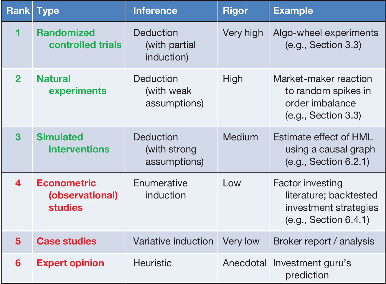
At the bottom of the hierarchy is the expert opinion, such as the discretionary view of an investment guru, which relies on rules of thumb and educated guesses (heuristics) to reach a conclusion. A case study proposes a rationale to explain multiple aspects of a phenomenon (variative induction), however it typically lacks academic rigor and suffers from confirmation or selection biases. An econometric (observational) study, such as an investment factor model or backtest, relies primarily on statistical patterns observed on numerous instances (enumerative induction). Econometric studies can be academically rigorous, however they are afflicted by the pitfalls explained in Section 6.4. These three associational types of evidence are highly susceptible to type-A and type-B spuriosity.
A simulated intervention is qualitatively different from the bottom three categories because it uses the formal language of causal inference to communicate a falsifiable theory. The deduced causal effects rely on the strong assumption that the causal graph is correct.Footnote 35 Natural experiments are yet superior to simulated experiments because the former involve an actual do-operation. The deduced causal effects rely on the weaker assumption that Nature’s assignment of units to the treatment and control groups has been random. Finally, the top spot belongs to RCTs, because they offer the greatest level of transparency and reproducibility. The deduced causal effects rely on the assumption that the underlying causal mechanism will continue to operate (a form of induction). At the present, controlled experiments on financial systems are not possible, due to the complexity of these systems, but also due to ethical and regulatory considerations.
The reader should not conclude from Figure 12 that associational evidence is useless. As explained in Section 3.1, associations play a critical role in the phenomenological step of the scientific method. Furthermore, the causal mechanism embedded in a theory implies the existence of key associations which, if not found, falsify the theory (see Section 3.3). In standard sequent notation, the claim that
 is not enough to assert
 , however it is enough to assert that
 , where
 stands for causation and
 stands for association. The reason is, causation is a special kind of association (i.e., the kind that flows through a causal path), hence the absence of association is enough to debunk the claim of causation by modus tollens.
Figure 12 does not include out-of-sample evidence as a category, because “out-of-sample” is not a type of causal evidence but rather a description of when the data was collected or used. Evidence collected out-of-sample is of course preferable to evidence collected in-sample, as the former is more resilient to type-A spuriosity, however evidence collected out-of-sample is not necessarily more resilient to type-B spuriosity. For example, a researcher may collect out-of-sample evidence of the correlation between stocks and bonds, and from that measurement be tempted to deduce that changes in one’s price cause changes in the other’s price. While a causal link between stocks and bonds would be a possible explanation for the observed association, the existence of correlation does not suffice to claim a direct causal relationship, regardless of whether the measurement was taken in-sample or out-of-sample.
7 Monte Carlo Experiments
As explained in Section 6.4.2, factor model specification errors can lead to false positives and false negatives. This section presents three instances of causal structures where the application of standard econometric procedures leads to mistaking association with causation, and ultimately to type-B spurious factor claims. Standard econometric procedures are expected to perform equally poorly on more complex causal structures.
7.1 Fork
Three variables
 form a fork when variable
 is a direct cause of variable
 and variable
 (see Figure 13). Consider a researcher who wishes to model
 as a function of
 . In that case,
 is said to be a confounding variable because not controlling for the effect of
 on
on
 and
and
 will bias the estimation of the effect of
 on
on
 . Given a probability distribution
 , the application of Bayesian network factorization on the fork represented by Figure 13 yieldsFootnote 36:
 (17)
(17)
which implies a (noncausal) association between
 and
and
 , since
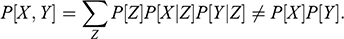 (18)
(18)
Causal graph with a confounder
 , before (left) and after (right) control
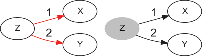
This is an example of noncausal association, because
 and
and
 are associated through the backdoor path
 , even though there is no causal path between
 and
and
 . The effect of conditioning by
 is equivalent to simulating a do-operation (an intervention), because it blocks the backdoor path, resulting in the conditional independence of
 and
and
 ,
,
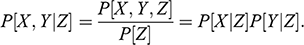
Conditioning by variable
 de-confounds
 in this causal graph, however not in other causal graphs. The widespread notion that econometricians should condition (or control) for all variables involved in a phenomenon is misleading, as explained in Section 6.4.2.2. The precise de-confounding variables are determined by do-calculus rules (see Section 4.3.2). The above conclusions can be verified through the following numerical experiment. First, draw 5,000 observations from the data-generating process characterized by the structural equation model,
 (20)
(20)
 (21)
(21)
 (22)
(22)
where
 are three independent random variables that follow a standard Normal distribution. Second, fit on the 5,000 observations the linear equation,
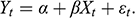 (23)
(23)
Figure 14 reports the results of the least-squares estimate. Following the econometric canon, a researcher will conclude that
 is statistically significant. Given the causal content injected by the researcher through the least-squares model specification, a statistically significant
 implies the statement “
 causes
 ,” not the statement “
 is associated with
 ” (Section 5.2). If the researcher intended to establish association, he should have used an associational model, such as Pearson’s correlation coefficient, or orthogonal regression (Section 5.1). At the same time, Figure 13 shows that there is no causal path from
 to
to
 . The claim of statistical significance is type-B spurious because
 is not a function of
 , as implied by the model’s specification. This is the effect of missing a single confounder.
False positive due to missing confounder

As explained in Section 6.4.2.1, it is possible to remove the confounder-induced bias by adding
 as a regressor (the partial correlations method),
 (24)
(24)
Figure 15 reports the result of this adjustment. With the correct model specification, the researcher will conclude that
 does not cause
 . The code for this experiment can be found in the Appendix.
De-confounding through the partial correlations method

7.2 Immorality
Three variables
 form an immorality when variable
 is directly caused by variable
 and variable
 (see Figure 16). Consider a researcher who wishes to model
 as a function of
 . In that case,
 is said to be a collider variable.
Causal graph with a collider
 , with (left) and without (right) control
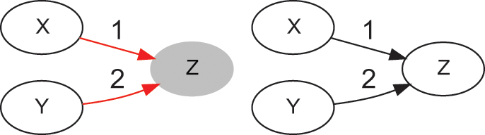
Colliders should be particularly concerning to econometricians because controlling for the effect of
 on
on
 and
and
 biases the estimation of the effect of
 on
on
 . Given a probability distribution
 , the application of Bayesian network factorization on the immorality represented by Figure 16 yields:
 (25)
(25)
There is no association between
 and
and
 because
 (26)
(26)
However, conditioning on
 opens the backdoor path between
 and
and
 that
that
 was blocking
 . The following analytical example illustrates this fact. Consider the data-generating process
 (27)
(27)
 (28)
(28)
 (29)
(29)
where
 are three independent random variables that follow a standard Normal distribution. Then, the covariance between
 and
and
 is
is
 (30)
(30)
The problem is, a researcher who (wrongly) conditions on
 will find a negative covariance between
 and
and
 , even though there is no causal path between
 and
and
 , because
 (31)
(31)
The Appendix contains a proof of the above proposition. Compare the causal graph in Figure 16 with the causal graph in Figure 13. Figure 13 has a structure
 , where not controlling for confounder
 results in under-controlling. The direction of causality is reversed in Figure 16, transforming the confounder into a collider. In the structure
 , controlling for
 results in over-controlling. This is an instance of Berkson’s fallacy, whereby a noncausal association is observed between two independent variables, as a result of conditioning on a collider (Reference PearlPearl 2009, p. 17).
This finding is problematic for econometricians because the direction of causality cannot always be solely determined by observational studies (Reference Peters, Janzing and ScholkopfPeters et al. 2017, pp. 44–45), and solving the confounder-collider conundrum often requires the injection of extra-statistical (beyond observational) information. Causal graphs inject the required extra-statistical information, by making explicit assumptions that complement the information contributed by observations.Footnote 37 Accordingly, the statistical and econometric mantra “data speaks for itself” is in fact misleading, because two econometricians who rely solely on observational evidence can consistently reach contradicting conclusions from the analysis of the same data. With a careful selection of colliders, a researcher can present evidence in support of any type-B spurious investment factor. The correct causal treatment of a collider is to indicate its presence and explain why researchers should not control for it. A key takeaway is that researchers must declare and justify the hypothesized causal graph that supports their chosen model specification, or else submit to the healthy skepticism of their peers.
We can verify the above conclusions with the following numerical experiment. First, draw 5,000 observations from the above data-generating process. Second, fit on the 5,000 observations the linear equation
 (32)
(32)
Figure 17 reports the results of the least-squares estimate. Following the econometric canon, a researcher will conclude that
 is statistically significant. This claim of statistical significance is type-B spurious because
 is not a function of
 , as implied by the model’s specification. This is the effect of controlling for a collider.
False positive due to adding collider


We can remove the bias induced by collider
 by excluding that variable from the model’s specification,
 (33)
(33)
Figure 18 reports the results of this adjustment. Note that the misspecified model delivered higher explanatory power, hence specification-searching would have misled the researcher into a false positive. With the correct model specification, the researcher will conclude that
 does not cause
 . The code for this experiment can be found in the Appendix.
Debiasing by removing collider

7.3 Chain
Three variables
 form a chain when variable
 mediates the causal flow from variable
 to variable
 (see Figure 19). Consider a researcher who wishes to model
 as a function of
 . In that case,
 is said to be a mediator variable.
Causal graph with mediator
 , before (top) and after (bottom) control
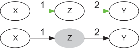
Given a probability distribution
 , the application of Bayesian network factorization on the chain represented by Figure 19 yields:
 (34)
(34)
which implies an association between
 and
and
 , since
 (35)
(35)
There is no backdoor path in Figure 19. This is an example of association with causation, because
 and Y are associated only through the causal path mediated by
 . Like in the case of a fork, the effect of conditioning by
 is equivalent to simulating a do-operation (an intervention), resulting in the conditional independence of
 and
and
 ,
,
 (36)
(36)
The problem with conditioning on a mediator is that it may disrupt the very causal association that the researcher wants to estimate (an instance of over-controlling, see Section 6.4.2.2), leading to a false negative. Making matters more complex, conditioning on a mediator can also lead to a false positive. This statement can be verified through the following numerical experiment. First, draw 5,000 observations from the data-generating process characterized by the structural equation model


 (38)
(38)
 (39)
(39)
 (40)
(40)
where
 are four independent random variables that follow a standard Normal distribution. Figure 20 displays the relevant causal graph.Footnote 38 Second, fit on the 5,000 observations the linear equation
 (41)
(41)
A confounded mediator (
 ), with (left) and without (right) control
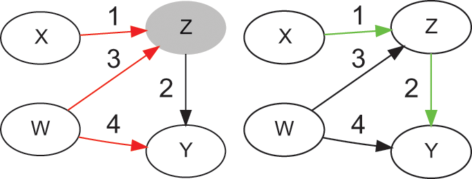
Figure 21 reports the results of the least-squares estimate. While it is true that
 causes
 (through
 ), this result is still a false positive, because the reported association did not flow through the causal path
 . The reason is,
 also operates as a collider to
 and
and
 , and controlling for
 has opened the backdoor path
 . This is the reason
 , despite of all effects being positive. This phenomenon is known as the mediation fallacy, which involves conditioning on the mediator when the mediator and the outcome are confounded (Reference Pearl and MacKenziePearl and MacKenzie 2018, p. 315). This experiment also illustrates Simpson’s paradox, which occurs when an association is observed in several groups of data, but it disappears or reverses when the groups are combined (Reference Pearl, Glymour and JewellPearl et al. 2016, pp. 1–6).
False positive due to adding a confounded mediator

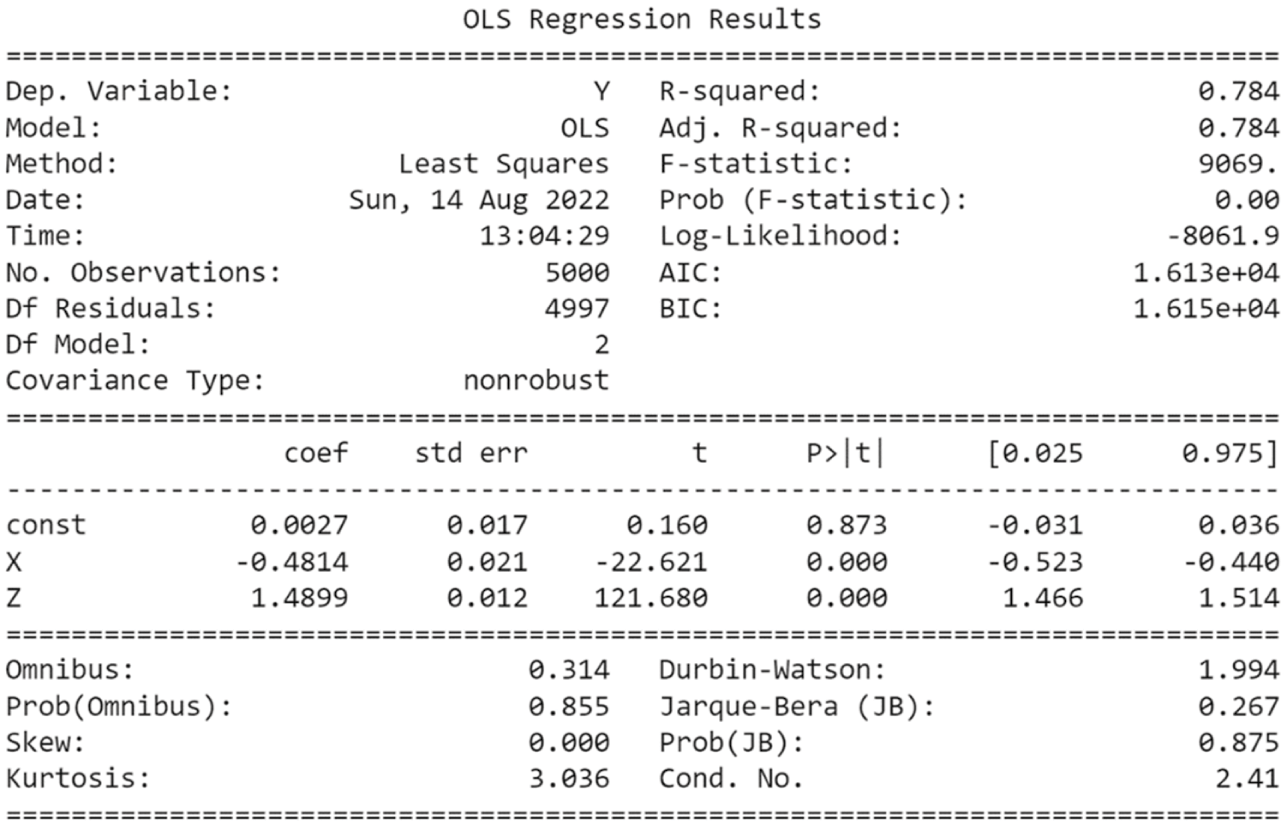
Following the rules of do-calculus, the effect of
 on
on
 in this causal graph can be estimated without controls. The reason is, the noncausal path through
 is already blocked by
 . Controlling for
 is not strictly necessary to debias
 , however it can help improve the precision of the estimates. The following model specification produces an unbiased estimate of
 :
:
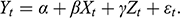
Figure 22 reports the results. Note that the correct model specification has much lower explanatory power: the adjusted R-squared drops from 0.784 to 0.144, and the F-statistic drops from 9,069 to 840.8. A specification-searching researcher would have chosen and reported the wrong model, because it has higher explanatory power, resulting in a misspecified model that misattributes risk and performance (Section 6.4.2.3).
De-confounding by removing the confounded mediator
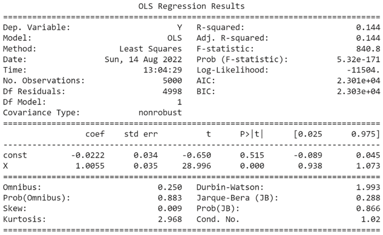
With the proper model specification, as informed by the declared causal graph, the researcher correctly concludes that
 causes
 , and that
 . The code for this experiment can be found in the Appendix.
7.4 An Alternative Explanation for Factors
Consider the influential three-factor and five-factor models proposed by Reference Fama and FrenchFama and French (1993) and Reference Fama and FrenchFama and French (2015). These journal articles, henceforth referred to as FF93 and FF15 respectively, have inspired and served as template for thousands of academic papers purporting the discovery of hundreds of factors. FF93 postulates that the cross-section of average stock returns is partly explained by a linear function of three factors, namely the broad market, size (quantified as stock price times number of shares), and value (quantified as book-to-market equity). FF15 added to this mix two quality-inspired factors, profitability and investment, on the premise of improving the model’s explanatory power. The model specifications proposed by FF93 and FF15 raise several objections: First, the authors fail to report and adjust for all the trials carried out before selecting their model, thus p-hacking has likely taken place (Section 6.4.1.1). Second, the authors justify the proposed specifications in terms of explanatory power, instead of a causal graph, thus the model is likely misspecified due to specification-searching (Section 6.4.2.3). Third, the authors ignore known macroeconomic confounders, such as inflation, GDP, stage of the business cycle, steepness of the yield curve, etc. Strangely, section 2.1.2 of FF93 makes explicit mention to the confounding effect of business cycles on size, and yet that confounder is inexplicably absent in the model. This points to a missing confounder (Section 6.4.2.1). Fourth, it is well documented that there is an interaction between the momentum and value factors (Reference Barroso and Santa-ClaraBarroso and Santa-Clara 2015). This interaction could be explained by a confounding relation between momentum and value, making momentum another likely missing confounding variable. Fifth, the authors do not provide the causal mechanism responsible for the reported observations, in denial of the causal content of their model, hence obstructing mediation analysis and falsification efforts (Section 6.3).
Reference CarhartCarhart (1997) (henceforth C97) expanded FF93 by adding momentum as a fourth factor; however, the justification for that expansion was that the four-factor model achieved higher explanatory power (an associational argument), not that controlling for momentum de-confounded the estimate of value’s causal effect. This is the same self-contradictory argument that FF15 used to add the two quality factors (Section 6.4.2.3). As demonstrated in Section 7.3, a correctly specified model can deliver lower explanatory power than a misspecified model on the same dataset. Improving on FF93’s explanatory power does not make C97’s model better specified, or its estimates less biased. Furthermore, the de-confounding control variable (momentum) is highly correlated with the confounded variable (value), thus exchanging confounder bias for multicollinearity. There are better ways of debiasing value’s causal effect estimate. Instead of the partial correlations method, authors could apply the backdoor adjustment (or some other do-calculus adjustment), in order to avoid the multicollinearity caused by the inversion of that covariance matrix.
There is a plausible sixth objection to the specification of FF93, FF15, and C97. Suppose that (1) a company’s stock returns and size are independent variables; and (2) both variables influence the company’s book-to-market equity (a collider). In this case, as explained in Section 6.4.2.2 and illustrated in Section 7.2, conditioning on book-to-market equity introduces a negative noncausal association between the two independent variables in (1). In other words, by adding book-to-market equity to their model specification, FF93, FF15, and C97 may have inadvertently induced a noncausal negative correlation between stock returns and size, making the size factor a false discovery.
The numerical experiments in Section 7 demonstrate that general causal structures can explain away the findings in FF93, FF15, and C97 as type-B spurious. Figure 23 provides an example of a causal graph under which the estimates in FF93, FF15, and C97 are biased by confounders and colliders. This particular graph may not be correct, however, the burden of proving it wrong belongs to the authors claiming the existence of investment factors. To address these concerns, those authors should make their models’ causal content explicit, declare the hypothesized causal mechanism, control for the missing confounders, and justify their belief that none of the chosen explanatory variables is a collider.
Example of a causal graph under which the findings in FF93, FF15, and C97 are biased
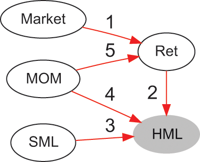
If FF93, FF15, and C97 had proposed a predictive model, producing such biased estimates of the factor coefficients would not be problematic, because the prediction might still lead to a profitable investment strategy. However, as explained in Section 6.1, the purpose of a factor model (such as FF93, FF15, and C97) is to build portfolios exposed to a particular risk characteristic presumably rewarded by the market. This is the reason value factor funds typically create a portfolio by ranking stocks in terms of their book-to-market ratio, not the model’s residuals.
To summarize, the findings in FF93, FF15, and C97 are likely type-A spurious, due to p-hacking, or type-B spurious, due to under-controlling of confounders, over-controlling of mediators, specification-searching, and missing mediation analysis. This is not a criticism of these three papers relative to the rest of the factor investing literature. On the contrary, with all their flaws, these three papers are as good as any other associational financial econometric study, and continue to be deeply influential. Other papers in this field share the same or similar methodological errors that make their promoted factors likely spurious.
8 Conclusions
A scientific theory is a falsifiable statement of the form “
 causes
 through mechanism
 .” Observed associations amount to phenomenological evidence, but do not rise to the status of scientific knowledge, for three reasons: (i) the observed association can be type-A spurious, due to p-hacking or backtest overfitting; (ii) even if true, the association is not necessarily causal; and (iii) even if causal, the association does not propose a falsifiable mechanism
 by which
 causes
 .
.
Scientific theories should matter to investors for at least three reasons: First, theories are a deterrent against type-A spuriosity, because they force scientists to justify their modelling choices, thus curtailing efforts to explain random variation (Section 6.4.1). A researcher who engages in p-hacking or backtest overfitting may build an ad hoc theory that explains an observed random variation. However, other researchers will use the theory to design an experiment where the original random variation is not observed (Section 3.3). Second, causality is a necessary condition for investment efficiency. Causal models allow investors to attribute risk and performance to the variables responsible for a phenomenon (Section 6.4.2). With proper attribution, investors can build a portfolio exposed only to rewarded risks, and aim for investment efficiency. In contrast, associational models misattribute risks and performance, thus preventing investors from building efficient portfolios. Third, causal models enable counterfactual reasoning, hence the stress-testing of investment portfolios in a coherent and forward-looking manner (see Reference RebonatoRebonato 2010; Reference Rebonato and DenevRebonato and Denev 2014; Reference DenevDenev 2015). In contrast, associational models cannot answer counterfactual questions, such as what would be the effect of
 on a not-yet-observed scenario
 , thus exposing those relying on associations to black-swan events.
Despite the above, the majority of journal articles in the investment literature make associational claims and propose investment strategies designed to profit from those associations. For instance, authors may find that observation
 often precedes the occurrence of event
 , determine that the correlation between
 and
and
 is statistically significant, and propose a trading rule that presumably monetizes such correlation. A caveat of this reasoning is that the probabilistic statement “
 often precedes
 ” provides no evidence that
 is a function of
 , thus the relationship between
 and
and
 may be coincidental or unreliable. One possibility is that variables
 and
and
 may appear to have been associated in the past by chance (type-A spuriosity), in which case the investment strategy will likely fail. Another possibility is that
 and
and
 are associated even though
 is not a function of
 (type-B spuriosity), for example due to a confounding variable
 which researchers have failed to control for, or due to a collider variable
 which researchers have mistaken for a confounder. These misspecification errors make it likely that the correlation between
 and
and
 will change over time, and even reverse sign, exposing the investor to systematic losses.
The main conclusion of this Element is that, in its current formulation, factor investing has failed to achieve its objectives. Academically, it is a data-mining exercise that has yielded countless type-A and type-B spurious findings. Commercially, it is falsely promoted as a scientific product, and it has failed to deliver statistically significant returns, against the profit expectations generated by its promoters.
To find the path forward, factor researchers must first understand how they ended up with a black-box. Part of the answer is the strong grip that commercial interests hold on financial academia. Financial academics interested in starting over on the more solid foundations of causal factor investing should pursue collaborations with the research arms of noncommercial asset managers, such as sovereign wealth managers and endowments.
8.1 Factor Investing Is a Black-Box
Virtually all journal articles in the factor investing literature deny or ignore the causal content of factor models. Authors do not identify the causal graph consistent with the observed sample, they justify their chosen model specification in associational terms (e.g., optimizing the coefficient of determination), and they rarely theorize a falsifiable causal mechanism able to explain their findings. Absent a causal theory, it is nearly impossible to falsify their claims thoroughly (Section 3). It could take decades to collect enough out-of-sample evidence to determine that the association is false, and in-sample evidence is highly susceptible to p-hacking and backtest overfitting. The outcome from a backtest or a factor model is yet another associational claim, prone to the same misunderstandings and spurious claims discussed in Sections 5 and 6. For example, the factor models and backtests of strategies based on FF93, FF15, and C97 do not prove that holding value stocks causes a portfolio to outperform the market, because that causal claim can only be tested by the methods described in Section 4. Even if it were true that holding value stocks causes a portfolio to outperform the market, neither a factor model nor a backtest tells us why.
Consider the large losses experienced by value funds between late 2017 and early 2022. Investors never received a straight answer to the question “why did value funds perform so poorly?” The reason is, in absence of a causal theory, nobody knows why value funds should have performed well in the first place, or what turned the sign of value’s
 (a hallmark of type-B spurious factors, see Section 6.4.2). Asset managers will not admit their confusion to clients, as that would invite large-scale redemptions. Answering the “why” question requires a falsifiable causal mechanism, which to this day remains unknown for value investments.
Due to the omission of causal mechanisms (Section 6.2), factor investment strategies are promoted like associational investment strategies, through inductive arguments. For example, a researcher may find that value and momentum strategies have been profitable for many years (enumerative induction) or in many different geographies (variative induction). This associational finding generates the expectation that, whatever the unknown cause of value and momentum, and whatever the mechanism responsible for their profitability, history will continue to repeat itself, even though there is no scientific-deductive basis for such belief. Ironically, commercial asset managers routinely require investors to accept disclaimers such as “past performance is not indicative of future results,” in direct contradiction with the inductive claims that authors promote and managers sell to customers.
Answering the “why” question is of particular importance for institutional investors, such as pension funds, sovereign wealth funds, endowments, and insurance companies. These investors manage funds for the benefit of the general public, and have a limited appetite for gambling. Factor investing may be an appropriate strategy for a high-net-worth individual, who can afford losing a large portion of his fortune. However, a salaried worker who has saved for 50 years and depends on those savings to retire should not be induced to wager his future wellbeing on investment strategies that, even if apparently profitable, are black-boxes. As long as asset managers remain unable to answer the “why” question, they should refrain from promoting to the general public factor investing products as scientific, and institutional investors should question whether factor investing products are investment grade.
8.2 The Economic Incentives for Associational Studies
In 2019, J.P. Morgan estimated that over USD 2.5 trillion (more than 20 percent of the US equity market capitalization) was managed by quant-style funds (Reference BermanBerman 2019). BlackRock estimates that the factor investing industry managed USD 1.9 trillion in 2017, and it projects that amount will grow to USD 3.4 trillion by 2022 (BlackRock 2017). This massive industry has been built on academic output, not on results for investors.
Reference HarveyHarvey (2022) argues that economic incentives, instead of scientific considerations, may be driving the academic agenda. The financial industry funds associational studies, because they are cheaper and easier to produce than causal (scientific) studies, while they help achieve annual revenues in the tens of billions of US dollars. Unless asset owners demand change, the academic establishment will dismiss the need for causality, just as it continues to dismiss the existence of a reproducibility crisis caused by rampant p-hacking and backtest overfitting, in defiance of warnings issued by the American Statistical Association, the American Mathematical Society, and the Royal Statistical Society, among other scientific bodies.
8.3 The Dawn of Causal Factor Investing
Answering the “why” question is more than an academic pursuit. Causal factor theories would be highly beneficial to all types of investors, for several reasons: First, efficiency: causal models attribute risk and performance correctly. With proper risk and performance attribution, researchers can build portfolios that concentrate exposure on rewarded risks and hedge unrewarded risks. Second, interpretability: every institutional investor owes it to its beneficial owners to explain why they may have to delay their plans (e.g., retirement). Third, transparency: a causal graph makes explicit all the assumptions involved in a theorized mechanism. Investment strategies based on causal theories are not black-boxes. Fourth, reproducibility: a causal explanation reduces the chances of (i) random variation (type-A spuriosity), by confining the search space to plausible theories, and (ii) noncausal association (type-B spuriosity), by providing some assurances that the phenomenon will continue to occur as long as the mechanism remains. Fifth, adaptability: the profitability of investment strategies founded on associational relations relies on the stability of the joint distribution’s parameters, which in turn depends on the stability of the entire causal graph (variable levels and parameters). In contrast, investment strategies based on causal relations are resilient to changes that do not involve the parameters in the causal path (see Section 6.4.2.1). This makes causal investment strategies more reliable than associational investment strategies. Sixth, extrapolation: only an investment strategy supported by a causal theory is equipped to survive and profit from black-swan events, by monitoring the conditions that trigger them (e.g., liquidity strategies based on the PIN theory performed well during the 2010 flash crash). Seventh, surveillance: the validity of a causal mechanism can be assessed in more direct and immediate ways than estimating the probability of a structural break in performance. This attribute is of critical importance in a complex dynamic system like finance: (i) an investor in a causal factor investing strategy may be able to divest when the causal mechanism weakens, before losses compound to the point that a statistical test detects a structural break; (ii) causal mechanisms enable factor timing, dynamic bet sizing, and tactical asset allocation. Eighth, improvability: causal theories can be refined, as a researcher learns more about the mechanism responsible for the observations. The fate of investment strategies based on causal theories is not unavoidable decay toward zero performance. These are all attributes that make an investment strategy appealing and trustworthy, and that current factor investments lack.
Financial economists’ adoption of causal inference methods has the potential to transform investing into a truly scientific discipline. Economists are best positioned to inject, make explicit, and argue the extra-statistical information that complements and enriches the work of statisticians. Financial economists interested in causal research would do well in partnering with noncommercial asset managers, such as sovereign wealth funds and endowments. These institutional investors are not conflicted by commercial interests, and their objectives are aligned with their beneficial owners.
The new discipline of “causal factor investing” will be characterized by the adaptation and adoption of tools from causal discovery and do-calculus to the study of the risk characteristics that are responsible for differences in asset returns. Every year, new alternative datasets become available at an increasing rate, allowing researchers to conduct natural experiments and other types of causal inference that were not possible in the twentieth century. Causal factor investing will serve a social purpose beyond the reach of (associational) factor investing: help asset managers fulfill their fiduciary duties with the transparency and confidence that only the scientific method can deliver. To achieve this noble goal, the dawn of scientific investing, the factor investing community must first wake up from its associational slumber.
Appendix
A.1 Proof of Proposition in Section 6.4.2.1
Consider a data-generating process with equations:
 (43)
(43)
 (44)
(44)
where
 ,
,
 , and variables
 are independent and identically distributed as a standard Normal,
 . The causal graph for this process is displayed in Figure 10 (bottom). The process is unknown to observers, who attempt to estimate the causal effect of
 on
on
 by fitting the equation
 on a sample produced by the process. Then, the expression
 is,
is,
 (45)
(45)
Replacing
 , we obtain
 (46)
(46)
Since the expected value is conditioned by
 , we replace
 to obtain

 (47)
(47)
Knowledge of
 does not convey information on
 , hence
 , however knowledge of
 conveys information on
 , since
 . Accordingly, we can reduce the above expression to
 (48)
(48)
This leaves us with an expression
 that we would like to simplify. Note that variables
 follow a Gaussian distribution with known mean and variance,
 (49)
(49)
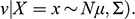
We can compute
 explicitly, using the formulas for the conditional Gaussian distribution (Reference EatonEaton 1983, pp. 116–117),Footnote 39
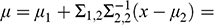
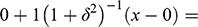
 (51)
(51)
For completeness, we can derive the variance
 as
as
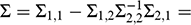
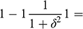
 (52)
(52)
Using the above results, the expression of
 reduces to,
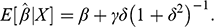 (53)
(53)
This completes the proof.
A.2 Proof of Proposition in Section 7.2
Consider the data-generating process with equations:
 (54)
(54)
 (55)
(55)
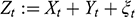 (56)
(56)
where
 are three independent random variables that follow a standard Normal distribution,
 . The random variable
 is still Gaussian,
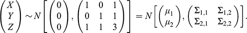 (57)
(57)
The conditional distribution has the form
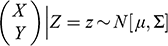
where the parameters can be derived using the formulas for the conditional Gaussian distribution (Reference EatonEaton 1983, pp. 116–117),
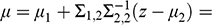
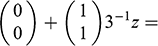
 (59)
(59)

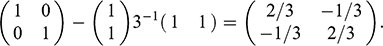 (60)
(60)
Then, the covariance between
 and
and
 conditional on
 is
is
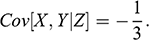 (61)
(61)
This completes the proof.
B.1 Code for Experiment in Section 7.1
Snippet 1 lists the Python 3 code used to produce the results of the Monte Carlo experiment that simulates a fork.
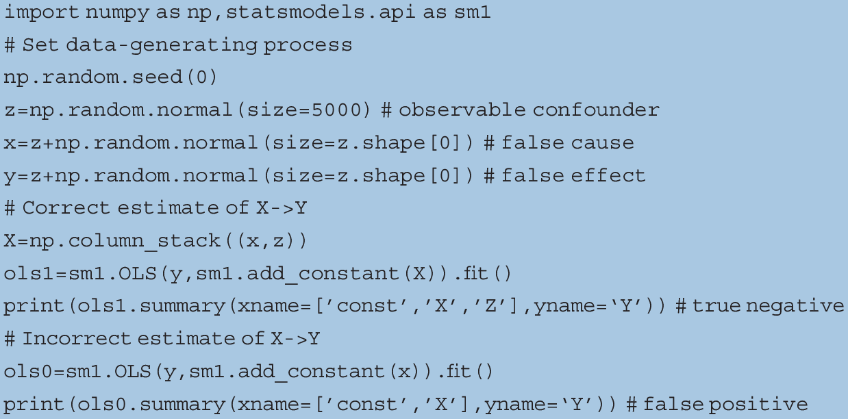
import numpy as np,statsmodels.api as sm1# Set data-generating processnp.random.seed(0)z=np.random.normal(size=5000) # observable confounderx=z+np.random.normal(size=z.shape[0]) # false causey=z+np.random.normal(size=z.shape[0]) # false effect# Correct estimate of X->YX=np.column_stack((x,z))ols1=sm1.OLS(y,sm1.add_constant(X)).fit()print(ols1.summary(xname=[’const’,’X’,’Z’],yname=‘Y’)) # true negative# Incorrect estimate of X->Yols0=sm1.OLS(y,sm1.add_constant(x)).fit()print(ols0.summary(xname=[’const’,’X’],yname=‘Y’)) # false positiveB.2 Code for Experiment in Section 7.2
Snippet 2 lists the Python 3 code used to produce the results of the Monte Carlo experiment that simulates an immorality.
import numpy as np,statsmodels.api as sm1# Set data-generating processnp.random.seed(0)x=np.random.normal(size=5000) # false causey=np.random.normal(size=x.shape[0]) # false effectz=x+y+np.random.normal(size=x.shape[0]) # collider# Correct estimate of X->Yols0=sm1.OLS(y,sm1.add_constant(x)).fit()print(ols0.summary(xname=[’const’,’X’],yname=‘Y’)) # true negative# Incorrect estimate of X->YX=np.column_stack((x,z))ols1=sm1.OLS(y,sm1.add_constant(X)).fit()print(ols1.summary(xname=[’const’,’X’,’Z’],yname=‘Y’)) # false positiveB.3 Code for Experiment in Section 7.3
Snippet 3 lists the Python 3 code used to produce the results of the Monte Carlo experiment that simulates a chain.
import numpy as np,statsmodels.api as sm1# Set data-generating processnp.random.seed(0)x=np.random.normal(size=5000) # causew=np.random.normal(size=x.shape[0]) # confounderz=x+w+np.random.normal(size=x.shape[0]) # mediatory=z+w+np.random.normal(size=x.shape[0]) # effect# Correct estimate of X->Yols1=sm1.OLS(y,sm1.add_constant(x)).fit()print(ols1.summary(xname=[’const’,’X’],yname=‘Y’)) # true positive# Incorrect estimate of X->YX=np.column_stack((x,z))ols1=sm1.OLS(y,sm1.add_constant(X)).fit()print(ols1.summary(xname=[’const’,’X’,’Z’],yname=‘Y’)) # false positiveAcknowledgments
The views expressed in this Element are the author’s, and do not necessarily represent the opinions of the organizations he is affiliated with. Special thanks are due to Majed AlRomaithi, Alexander Lipton, Jean-Paul Villain, and Vincent Zoonekynd, for numerous comments and contributions. The Element has also benefited from conversations with more ADIA colleagues than I can cite here, as well as Victoria Averbukh (Cornell University), David H. Bailey (Berkeley Lab), David Easley (Cornell University), Frank Fabozzi (EDHEC), Campbell Harvey (Duke University), John Hull (University of Toronto), Alessia López de Prado Rehder (ETH Zurich), Maureen O’Hara (Cornell University), Emilio Porcu (Khalifa University), Riccardo Rebonato (EDHEC), Alessio Sancetta (Royal Holloway, University of London), Luis Seco (University of Toronto), Sasha Stoikov (Cornell University), Josef Teichmann (ETH Zurich), and Jorge Zubelli (Khalifa University).
I would like to express my gratitude to the members of ADIA Lab’s Executive Board, for supporting the publication of this Element as Open Access: Abdulla AlKetbi (Chair), Fatima Almheiri (Vice-Chair), Khamis AlKhyeli, Humaid AlKaabi, Ahmed Almheiri, and Marwan AlRemeithi.
Finally, ADIA Lab’s Advisory Board comprises esteemed colleagues who are a constant source of inspiration: Horst Simon (Director), Steven Chu (Stanford University), Jack Dongarra (University of Tennessee), Shafi Goldwasser (UC Berkeley), Miguel Hernán (Harvard), Edward Jung (Intellectual Ventures), Alexander Lipton (Hebrew University), and Alexander Pentland (MIT).
Marcos López de Prado is Global Head of Quantitative Research and Development at the Abu Dhabi Investment Authority, a founding board member of ADIA Lab, and Professor of Practice at Cornell University’s School of Engineering, where he teaches machine learning. In recognition of his work, Marcos has received various scientific and industry awards, including the National Award for Academic Excellence (1999) by the Kingdom of Spain, the Quant Researcher of the Year Award (2019) by The Journal of Portfolio Management, and the Buy-Side Quant of the Year Award (2021) by Risk.net. For more information, visit www.QuantResearch.org
About ADIA Lab
ADIA Lab is an independent institution engaged in basic and applied research in Data Science, Artificial Intelligence, Machine Learning, and High-Performance Computing, across all major fields of study. This includes exploring applications in areas such as climate change and energy transition, blockchain technology, financial inclusion and investing, decision making, automation, cybersecurity, health sciences, education, telecommunications, and space.
Based in Abu Dhabi, ADIA Lab is an independent, standalone entity supported by the Abu Dhabi Investment Authority (ADIA), a globally-diversified investment institution that invests funds on behalf of the Government of Abu Dhabi.
ADIA Lab has its own governance and operational structure, and is guided by an Advisory Board of global thought-leaders in data and computationally-intensive disciplines, including winners of the Nobel, Turing, Gödel, Rousseeuw, Gordon Bell, and other prizes.
Riccardo Rebonato
EDHEC Business School
Editor Riccardo Rebonato is Professor of Finance at EDHEC Business School and holds the PIMCO Research Chair for the EDHEC Risk Institute. He has previously held academic positions at Imperial College, London, and Oxford University and has been Global Head of Fixed Income and FX Analytics at PIMCO, and Head of Research, Risk Management and Derivatives Trading at several major international banks. He has previously been on the Board of Directors for ISDA and GARP, and he is currently on the Board of the Nine Dot Prize. He is the author of several books and articles in finance and risk management, including Bond Pricing and Yield Curve Modelling (2017, Cambridge University Press).
About the Series
Cambridge Elements in Quantitative Finance aims for broad coverage of all major topics within the field. Written at a level appropriate for advanced undergraduate or graduate students and practitioners, Elements combines reports on original research covering an author’s personal area of expertise, tutorials and masterclasses on emerging methodologies, and reviews of the most important literature.


 Open access