


Introduction
Renewable energy technologies have seen considerable adoption over the last few decades (EIA, 2019c). Certain renewables, such as wind and solar power, are particularly unique technologies in that the amount of energy they supply is intermittent. Specifically, by intermittent, we mean that their output changes in predictable ways related to physical constraints. For example, wind turbine output varies with wind speed and direction, which can be predicted ahead of time. On the other hand, traditional fossil fuel energy sources offer a constant amount of energy. Intermittency presents a challenge when evaluating the economic value of renewable energy. Traditional approaches such as the levelized cost of electricity (LCOE) fail to capture the true economic value of intermittent technologies, because they neglect to account for variation in output and prices over time (Joskow Reference Joskow2011). Additionally, the intermittency of renewables complicates their ability to substitute for fossil energy, because consumers prefer to have more electricity at certain times than others, while the output of intermittent renewables varies exogenously with the weather. Consequently, modeling and better understanding the effects of intermittency would help us design more effective policies to promote the adoption of renewable energy.
In this article, we develop a partial equilibrium model of the electricity sector that takes into account intermittent generation. Specifically, the electricity sector consists of a representative firm that chooses and builds capacity from a set of electricity-generating technologies to maximize profit; some of these technologies are intermittent, while others are consistent. Then, we consider a representative consumer who purchases varying quantities of electricity in each period in order to maximize utility. People prefer to smooth their electricity consumption over time, so we model our consumer's preferences using a CES function of electricity consumption and assume preferences are time dependent.Footnote 1 These two sides of the market reach an equilibrium through the prices of electricity in each period.
Our model has two important features that distinguish it from present approaches in the literature. Firstly, it accommodates the critique made by Joskow (Reference Joskow2011). In our model, when firms maximize profit, they implicitly measure the economic value of each energy technology by integrating its production profile with electricity prices. That is, firms take into account how much a technology produces in each period and the price of electricity in those periods, as opposed to simply taking the product of the average electricity output of a technology with the average price of electricity. Secondly, our model captures the imperfect substitutability of intermittent and reliable energy technologies by modeling consumers with a preference for smooth electricity consumption, which they signal through prices. When firms respond to this signal and maximize profit, the equilibrium result is that the intermittency of certain renewables interferes with their ability to perfectly substitute for reliable energy technologies; that is, the substitutability of energy technologies is directly linked with their intermittency. This contrasts with alternative approaches that model electricity as a homogenous good produced according to a CES function of electricity-generating technologies; such approaches model imperfect substitutability on the supply side to implicitly capture the effects of intermittency. However, these approaches abstract from key features of intermittency and thus may reach incorrect conclusions.
Next, we parametrize our model empirically by fitting the parameters of the consumer's utility function using electricity consumption and price data for each U.S. state. Since the consumer's CES utility function is composed of electricity consumption differentiated by time, the elasticity parameter represents the intertemporal elasticity of substitution for electricity consumption; this parameter plays a particularly important role in our model, since it captures the effects of intermittency on demand. We also consider parametrizations of our model using previous estimates of this elasticity from the literature. Next, to model the supply side, we narrow our framework to a two-period, two-technology setting to focus on the substitutability between renewable and fossil energy. We proxy for renewable and fossil energy using solar and coal, respectively, while parametrizing each accordingly. Finally, we implement our model numerically and provide suggestions for policy and future models.
Our results quantify the relationship between the intertemporal elasticity of substitution for electricity consumption (IES) and the elasticity of substitution between renewable and fossil energy. The intuition behind the relationship is based on how the IES affects the desire for smoother consumption. When the IES is low, consumers want their electricity consumption to be smooth, so they prefer not to consume intermittent sources of energy such as solar. This means that the substitutability between renewables and fossils will be small. On the other hand, when the IES is high, consumers care less about smoothing their electricity consumption, so they are more willing to substitute between renewable and fossil energy. In short, the elasticity of substitution between renewable and fossil energy increases with the IES.
Furthermore, our numerical results show that the elasticity of substitution between renewable and fossil energy is non-constant and rises with the intermittency of present electricity generation. This occurs because consumers prefer to smooth their electricity consumption, so when electricity output varies more over time, it becomes harder to replace consistent technologies with intermittent technologies. The result that the elasticity of substitution between technologies is non-constant is important because a significant amount of literature has assumed a CES structure between renewable and fossil energy (see Papageorgiou, Saarn, and Schulte (Reference Papageorgiou, Saarn and Schulte2017)); this assumption has been motivated, in part, by the need to capture imperfect substitutability between these two generation technologies as a result of intermittency. However, our model finds that intermittency itself causes a non-constant elasticity between technologies. This elasticity appears to vary with the unit cost of each energy technology. Thus, we argue against assuming a CES structure. Alternatively, we argue that a variable elasticity of substitution (VES) production function should be used to approximate the relationship between the elasticity of substitution and the unit cost of each technology.Footnote 2 The numerical results suggest this relationship is roughly linear, which is exactly what a VES function assumes. Moreover, a VES function is analytically tractable, so it can be implemented in other frameworks without making them overly complicated.
These results have multiple important implications for environmental/energy policy. Firstly, the welfare burden of both a carbon tax and renewable subsidies varies geographically. This variation is a consequence of differences in the intermittency and availability of renewable energy by location. Moreover, this variability can create a trade-off between equity and efficiency when introducing policy to mitigate climate change. Secondly, we find strong motivation for research and development subsidies aimed at improving battery technology. Better energy storage can greatly increase the substitutability of renewable and fossil energy. Also, batteries can lessen the distributional side effects of carbon taxes and renewable subsidies by reducing intermittency. Thus, research into improving batteries can complement other policies by making them more equitable and by increasing their impact on the adoption of renewables. Finally, we revisit the results of Acemoglu et al. (Reference Acemoglu, Aghion, Bursztyn and Hemous2012) and qualitatively discuss the implications of our model in their setting.
Some of the literature has approached the question of intermittency by constructing numerical models that find the cheapest renewable technology set while accounting for intermittent supply. For instance, Musgens and Neuhoff (Reference Musgens and Neuhoff2006) model uncertain renewable output with intertemporal generation constraints, while Neuhoff, Cust, and Keats (Reference Neuhoff, Cust and Keats2007) model the temporal and spatial characteristics of wind output to optimize its deployment in the UK. Other articles study how intermittent technologies affect the market itself; Ambec and Crampes (Reference Ambec and Crampes2012) study the interaction between intermittent renewables and traditional reliable sources of energy in decentralized markets, and Chao (Reference Chao2011) models alternative pricing mechanisms for intermittent renewable energy sources. Additionally, Borenstein (Reference Borenstein2012) reviews the effects of present public policies used to promote renewables and the challenges posed by intermittency. Our model comes closest to that of Helm and Mier (Reference Helm and Mier2019), who build a peak-load pricing model where the availability of renewable capacity varies stochastically. Like Helm and Mier, we model the equilibrium of a market with dynamic pricesFootnote 3 and access to both renewable and fossil energy. However, Helm and Mier's approach is closer to one of reliability rather than intermittency. In accordance with the U.S. Department of Energy's ORNL (2004), reliability captures stochastic variability of electricity supply, while intermittency captures deterministic differences over time.Footnote 4 Consequently, since we model a different characteristic of renewable output, our model and results differ in a key way.
The remainder of the article proceeds as follows. The “Electricity Market Equilibrium” section states the consumer and firm problems and the resulting equilibrium. We also provide a discussion of the (consumer side) IES parameter and how it affects the optimal choice of electricity-generating inputs. Then, using estimable equitions based on the analytic results from the market equilibrium, we estimate the IES parameter. Next, in the Elasticity of Substitution section, we empirically parametrize and numerically implement our model. We also elaborate on the link between the IES parameter, intermittency, and the substitutability of renewable and fossil energy. In the Environmental and Energy Policy Implications section, we detail our model's policy implications. Finally, the Conclusion summarizes our article and offers suggestions for future models of intermittent renewables.
Electricity Market Equilibrium
Model
Consumers: Consumers purchase a quantity of electricity Z t in each period t. Furthermore, they demand a greater quantity of electricity in certain periods; for instance, consumers need more electricity during the middle of the day more than at night. At the same time, consumers are willing to shift their consumption from one period to another in response to a shift in prices. Overall, these characteristics can be captured using a standard CES utility function. Hence, we consider a representative consumer with the utility function

where σ = 1/(1 − ϕ) is the intertemporal elasticity of substitution for electricity consumption. The restriction on ϕ implies we have σ > 0; additionally, since electricity consumption increases utility, we must have α t > 0 for all t. For simplicity, we also define $\sum _t\alpha _t = 1$ , so that a 1 percent increase in electricity consumption in all periods increases utility by 1 percent; consequently, we then have α t ∈ (0, 1). The budget constraint is given by

where p t is the price of electricity in period t and I is the income. Our representative consumer maximizes utility against this budget constraint; the first order conditions of this problem imply:


where P is the price index. Note that this model naturally does not allow for blackouts in equilibrium, since the price of electricity in any period gets arbitrarily large as the quantity of energy consumed in that period approaches 0. Furthermore, note that prices must be positive; although this is sometimes violated in reality, we do not believe that this assumption significantly affects our analysis.
Firms: Secondly, we have firms maximizing profit by picking an optimal set of energy inputs. In reality, electricity markets are fairly competitive, so we can model the set of firms by using a single representative firm that sets marginal revenue equal to marginal cost.
We let X i represent the quantity of energy technology i, and we define its output per unit in period t as ξ 1,t. So, for example, if i is solar power, X i would be the number of solar panels and ξ i,t may be kWh generated per solar panel in period t. Consequently, the energy generated in period t, Z t, is given by $\sum _i\xi _{i\comma t}X_i$ . To simplify notation, we have

where we have n technologies, m periods, and Z ≡ ξTX.
A key assumption of our model is that the time scale is short enough such that the input vector X does not vary with time and the output per unit matrix ξ is exogenous. This is important because the time scale of our model must be fairly granular to study the effects of intermittency. So, for instance, a reasonably short two-period setting would be t ∈ {peak, off-peak}. Since the overall time frame is a single day, producers cannot modify the quantity of the technologies they deploy, so X must be fixed. Furthermore, this time frame is short enough to assume that ξ is exogenous; that is, technologies like coal power cannot significantly modify their output within a day, so ξ can be treated as a given set of constants. These two implications, that X cannot change over time and that ξ is exogenous, are important for parsimony, because they prevent more complicated dynamics from entering our model. And, they also make intermittency economically relevant, because having X fixed and ξ exogenous means that producers have no way of compensating for intermittent output; therefore, they must view the intermittency of technologies like solar and wind as a trade-off.
Furthermore, assuming a short time scale makes it simple to differentiate intermittent technologies. In this setting, we define an intermittent technology as a technology where output per unit varies with t. Specifically, this variation is exogenous and captured through ξ. We further narrow our article to deterministic variation as opposed to stochastic variation; hence, elements of the matrix ξ are constants. In total, we only need to consider ξ to determine whether a technology is intermittent. Additionally, in this context, we define intermittency as variation in electricity output over time. Since the set of inputs X are fixed over time, we can know whether the overall supply of electricity is intermittent based on total output Z = ξTX.
Now, we consider the firm's problem. Our representative firm chooses X to maximize total profit; it does so by setting marginal profit equal to marginal cost. Helm and Mier (Reference Helm and Mier2019) note that past literature has argued for concave cost functions in the energy market due to effects such as economies of scale and learning-by-doing; on the other hand, standard cost functions are generally convex. So, like Helm and Meir, we take an intermediate approach by using a linear cost function. Specifically, the total cost of the input bundle X is given by $\sum _ic_iX_i\equiv {\bi c}^T{\bi X}$ where c i is the cost per unit of X i. Then, total profit is given by

To simplify the algebra, we set the number of technologies equal to the number of periods (n = m). Additionally, we further require that the output per unit of each technology is unique and nonnegative in each period; in other words, the output per unit of one technology is not a linear combination of those of the other technologies in our set. This then implies that ξ is of full rank and therefore invertible. Now, maximizing profit, we find the first order condition:

Combining this FOC with the demand equation (equation 3) allows us to find the equilibrium. Generally, the equilibrium results for any number of technologies (n) are analytic, but they are difficult to interpret algebraically due to the number of parameters involved.
Equilibrium
For more tractable results, we consider a simpler scenario where n = m = 2 and σ = 1 (Cobb-Douglas); this particular case is described in greater detail in Appendix A.A. These assumptions simplify the discussion of intermittency. In a two-period, two-technology model, we can intuit that the magnitude of intermittency is given by how much ξ i,t/c i (output per dollar) varies with t; this is useful for understanding the link between intermittency and other parameters like σ. Furthermore, as we will discuss in our results, assuming σ = 1 is not far from its empirical estimate.
We define two recurring terms in our analysis: cost-efficiency and output efficiency in period t. For period t and technology i, we use cost-efficiency to refer to ξ i,t/c i and output efficiency to refer to ξ i,t. So, for example, with two technologies i and j at period t, technology i is more cost-efficient than technology j when ξ i,t/c i > ξ j,t/c j. Additionally, we say a technology is economical if its equilibrium quantity is above 0.
In Lemma 1 we use these two terms to define conditions that avoid an edge-case solution.
Lemma 1 Assume that, for all technologies i and periods t, we have ξ i,t > 0, α t > 0, and c i > 0. Then, for technology j to be economical, there need to exist a period s where the following three conditions are met:
ξ j,s/c j > ξ i,s/c i for all i
ξ j,s/ξ j,t > ξ i,s/ξ i,t where i ≠ j and t ≠ s
Period s demand needs to be sufficiently large, i.e., α s is large enough
The first condition is on cost-efficiency and is intuitive. Consider its contrapositive: if a technology does not have an advantage in cost-efficiency in any period, it will not be used. Alternatively, if a technology is the most cost-efficient in every single period, it will be the only technology used. The second condition regarding output stems from the invertibility of ξ. If we did not have ξ invertible, we either have at least one technology that does not produce in any period or we have at least one technology being a linear combination of the other technologies in terms of output and ξ is of row rank n < m, implying that at most, n technologies are used in equilibrium. Finally, the intuition behind the demand condition is straightforward; even if a technology is optimal in a certain period, if consumers do not sufficiently demand electricity during that period, then there is little reason to use that technology.
We may also derive the comparative statics for this simplified scenario.
Proposition 1 Suppose that the conditions of Lemma 1 hold for each technology, so we are not in an edge case. Then, the following hold:
The equilibrium quantity of a technology is increasing with its output and decreasing with its cost; at the same time, it is decreasing with the output of other technologies and increasing with the cost of other technologies.
Suppose that some technology i is the most cost-efficient in period t. Then, its equilibrium quantity is increasing with respect to the demand parameter α t and decreasing with respect to the demand parameters in other periods.
Furthermore, again assuming technology i is the most cost-efficient in period t, the comparative statics of Z t and X i are equivalent.
The comparative statics with respect to X i and output efficiency and cost of technology i are straightforward. On the other hand, the statics for Z t follow from the fact that we have Z ≡ ξTX. That is, suppose technology i is the most cost-efficient source of electricity in period t. If consumers demanded that 100 percent of their energy arrive in period t, then relying solely on technology i for energy would be the most economical solution. Consequently, the comparative statics of X i follow through to Z t. This intuition can then be generalized to when multiple technologies are employed and there is demand for electricity in multiple periods. Similarly, the comparative statics for the share parameters of the utility function, ${\bi \alpha }\equiv \lpar {\alpha_t \alpha_s} \rpar ^T$ , travel in the opposite direction. A rise in α t would directly raise the optimal quantity of Z t; hence, whichever technology is most cost-efficient at producing in period t would be used more. We provide a more detailed and formal discussion of the comparative statics and edge cases in Appendix A.
These theoretical results assumed σ = 1. This simplification implies that the utility function is Cobb-Douglas, which then results in the first-order condition Z t = α t/p t. This condition facilitates the analysis of ${\vector X}$ . In the following section, we empirically estimate σ to parametrize the model. Since the empirical estimate is not exactly 1, this complicates the solution for Z; consequently, the solution for X loses tractability. However, we can study the model analytically when σ is asymptotically large and small to see how it affects the equilibrium.
Proposition 2 Suppose that we have σ → ∞. Then,
Electricity consumption in each period t is a perfect substitute for electricity consumption in period s for all periods t, s;
The utility function takes on the linear form $U = \sum _t\alpha _tZ_t$ ; and
; and
The set of optimal bundles of inputs X is given by $W = \lcub {{\bi X}\colon {\bi c}^T{\bi X} = I\comma \;{\bi X}&InLnBrk;{\rm \;non}\hbox{-}{\rm negative}\comma \;{\rm and} \ \lpar {x_i \gt 0\Rightarrow i\in S} \rpar \forall i} \rcub$
${\rm where}\;S = \mathop {{\rm arg}\;{\rm max}}\limits_i \;\mathop \sum \limits_t \alpha _t\xi _{i\comma t}/c_i$
S represents the set of indices for technologies that have maximal cost-adjusted marginal utility. In other words, any vector of inputs X consisting of a feasible (non-negative X) and affordable (cTX = I) combination of technologies in S represents a valid equilibrium solution. Furthermore, the set $Y = \lcub {{\bi Z}\,\colon \,{\bi Z} = {\bi \xi }^T{\bi X}\forall {\bi X}\in W} \rcub$ contains all possible equilibrium values of electricity output.
A detailed proof of Proposition 2 is given in Appendix A.A.
If σ → ∞, then electricity consumption in each period becomes a perfect substitute for electricity consumption in other periods. In this case, the marginal utility of each input is $\sum _t\alpha _t\xi _{i\comma t}$ ; hence, the input that offers highest cost-adjusted marginal utility $\lpar {1/c_i} \rpar \sum _t\alpha _t\xi _{i\comma t}$
 will maximize utility. The perfect substitutability of Z t implies that consumers do not care about smoothing their electricity consumption over time. But they still value consumption in particular periods more than others through the α parameter. Consequently, they simply use whatever technology gives them the most total electricity (weighted by α). And there may be multiple technologies that maximize consumer utility in this way, so any combination of these technologies, indexed by S in Proposition 2, will be optimal.
Furthermore, since only total electricity output weighted by α matters when choosing the optimal set of inputs, there is no preference for smoothing electricity consumption over time; again, this is because σ → ∞ corresponds to the case of perfect substitutes. Consequently, the intermittency of an input has no effect on its adoption. This makes different inputs stronger substitutes for one another. To better understand why, suppose we have two technologies that cost the same per unit and produce the same total amount of electricity; one technology only produces during peak hours and the other producers only during the off-peak. If we have α peak = α off−peak, both technologies are perfect substitutes for one another when σ → ∞. This is because any feasible combination of the technologies would give the same utility to the representative consumer. For instance, using the first technology and only getting electricity during peak hours would offer the same amount of utility as using a mix of both technologies and getting electricity during both periods. On the other hand, if we had finite σ, consumers would care about having electricity during both periods. This would cause the equilibrium solution to involve using both inputs. So, in general, when σ → ∞, intermittency does not matter and inputs are more substitutable.
On the other hand, suppose that σ → 0; here, electricity consumption in each period is perfectly complementary with that in other periods. Furthermore, the utility function becomes $U = \mathop {\min }\limits_t \;Z_t/\alpha _t$ . While the analytic solution is not as clear here, some of the intuition from before carries through. As a result of perfect complementarity, consumers care strongly about smoothing their consumption. For instance, consider again a two-period, two-technology case with solar (intermittent) and coal (constant-output). Also, suppose that α t is constant. The utility function here implies that consumers only care about periods when they are getting the least electricity. Since solar performs worse during the off-peak, the implicit demand for solar would solely be based on its off-peak performance. Interestingly, no matter how high solar's output efficiency is during peak hours, the consumer's decisions and utility would be unaffected. On the other hand, when we had σ → ∞, the reduced performance of solar in the off-peak could always be compensated for by increasing performance during peak hours. In other words, intermittency plays a much larger role when σ → 0, since, in this case, a technology that with low output efficiency in certain periods cannot compensate by having higher output efficiency in other periods. This makes intermittent and consistent technologies weaker substitutes.
To summarize, the channel by which σ affects the inputs X is through the demand for electricity. Specifically, σ is inversely related to how much consumers value smoother electricity consumption Z. When σ is low, consumers care more about consumption smoothing. They are willing to reduce their total consumption of electricity if it means having more consistent electricity over time. In this case, intermittent energy technologies are less appealing because, by definition, they do not generate a consistent electricity output over time. On the other hand, when σ is high, consumers care less about consumption smoothing and are focused more on total consumption. In the extreme case above, when σ → ∞, they only care about total consumption and not about when they get their electricity. Intermittency becomes less of a concern, while other factors like cost-efficiency and output play a larger role. In short, σ is inversely related to how much the intermittency of an input matters.
Empirical Methodology
In order to better understand the practical implications of our model, we empirically estimate its parameters and study its implications numerically. We are particularly interested in estimating σ, since it determines the importance of intermittency. As shown earlier, when σ is large, consumers care less about when they get their electricity and are thus more likely to adopt intermittent technologies. On the other hand, when σ is small, consumers prefer to smooth their electricity consumption and therefore prefer less intermittent sources. Hence, ensuring that we have accurate estimates of σ is important for understanding how consumers decide between fossil and renewable energy. The other parameters in our model, c, ξ, and α are of secondary interest, since they are easier to obtain directly.
Recall the demand equation from earlier

where P is the price index and I is income. Retail customers pay fixed rates each month for electricity, hence p t is constant within each month, and we expect that income I does not vary significantly on a daily basis. Consequently, all variation in intramonthly demand is due to the share parameter α and the elasticity σ. But this creates a problem; since retail consumers do not face prices that vary each hour, we cannot estimate σ on an hourly basis.
A number of other articles have approached this problem using data from real-time pricing experiments.Footnote 5 In such experiments, consumers of electricity face prices that vary on an hourly basis; this makes it possible to estimateσ. Articles that use these experiments include Schwarz et al. (Reference Schwarz, Taylor, Birmingham and Dardan2002), Herriges et al. (Reference Herriges, Baladi, Caves and Neenan1993), and King and Shatrawka (Reference King and Shatrawka1994). The latter two articles estimate σ to be around 0.15 while the article by Schwarz et al. obtains estimates around 0.03. All three articles study real-time electricity pricing programs for industrial consumers using similar methodologies. Additionally, Aubin et al. (Reference Aubin, Fougere, Husson and Ivaldi1995) also provide estimates of the σ but using a different methodology; their results find an elasticity of substitution below 0. Under a CES structure, this is problematic, because it would imply upward-sloping demand curves. Finally, Mohajeryami et al. (Reference Mohajeryami, Moghaddam, Doostan, Vatani and Schwarz2016) also empirically estimate the share parameters for a CES function of this form, but they do not estimate the elasticity of substitution.
Overall, the past literature has estimated σ by running regressions on the CES demand equation, but we are concerned that this approach suffers from endogeneity. That is, producers may intertemporally substitute electricity output, which essentially means that there is a supply equation affecting prices. For instance, during the oil crisis of 1973, refineries increased gasoline stocks, expecting future prices to be higher (Adelman Reference Adelman1995). The existence of such behavior implies that estimates of σ would be biased downward unless we properly control for endogeneity. This is particularly important because whether σ is closer to 0.1 or 1 significantly changes the practical implications of our model.
So we take a different approach by using a supply instrument to identify the CES demand parameters. Specifically, we use coal prices, which affect the supply of electricity but not the demand. Furthermore, we estimate σ on a monthly basis. This decision is primarily due to data limitations, since we do not have access to the proprietary data on real-time pricing experiments, which the past literature has used. Although we are interested in understanding intertemporal substitution over a shorter time scale (since intermittency plays a larger role in shorter periods), estimates of σ on a monthly basis may still be applicable on a smaller time frame. For instance, Schwarz et al. (Reference Schwarz, Taylor, Birmingham and Dardan2002) estimate σ on a daily and hourly basis and find fairly close results; similarly, Herriges et al. (Reference Herriges, Baladi, Caves and Neenan1993) also find no significant difference in their estimates of σ for these two intervals. That is, while a daily basis is 24 times larger than an hourly basis, the estimates for σ, surprisingly, do not appear to change. Hence, we expect our estimates of σ on a monthly basis to not be far from estimates on shorter time scales. At the same time, our estimates of σ will likely be larger than that of the literature, because we are controlling for endogeneity. We now define our econometric methodology in detail.
Theory: We begin with the demand equation from our general model:


For any pair of electricity outputs Z t and Z s, we have:

Taking logs on both sides and letting i represent different observations, we may rewrite this in a form more suitable for estimation.

Our data differentiates consumption for each state in the United States, so we let i refer to a particular state. Additionally, most consumers pay monthly fixed rates for electricity, so we can, at most, estimate this equation on a monthly basis; hence, t and s refer to different months. Also, note that each observation only corresponds to a single state i; this is because consumers within each state can substitute consumption across time, but consumers in different states do not substitute consumption with one another.
In order to estimate this σ, we further modify this equation. Firstly, note that we cannot observe the demand shifter α t,i directly, so we must replace the α terms with a set of controls that may be responsible for shifts in demand. So, still in general terms, our regression equation is now

where A represents set of controls for changes in demand while u i is a normal error term. Note that the control A t,i replaces σln(α t,i) and likewise for the period s term; this substitution is valid because the ln(α t,i) ∈ ℝ and the σ term is simply absorbed into the estimated coefficient γ t,i. For the demand controls themselves, we consider degree days and the difference in months between periods t and s. Firstly, we use degree days rather than temperature due to the aggregation of the data. A degree day is defined as the difference between the average temperature for a day and a base temperature—our data uses 65°F (18°C). Cooling degree days (CDDs) and heating degree days (HDDs) further split this measure into deviations above and below the base temperature. That is, if the average temperature of a day is x°F, its CDD is max{0, x − 65} and its HDD is max{0, 65 − x}. Since these measures are linear, CDDs and HDDs can be aggregated without losing information. This does not hold true for temperature; averaging temperature over a month causes daily variation to be lost. Secondly, the demand for electricity may rise over time. Hence, we include, as a control, the difference in months between time t and s; this is represented by Δt,s. Finally, this panel requires us to consider fixed effects for each state, so we use a fixed effects panel regression. In total, the demand equation is:

Still, this equation may suffer from bias, since producers can also substitute production over time. To address endogeneity concerns, we define the following supply equation

where C t,i is the average cost of coal used for electricity generation in state i at time t and v i is a normal error term. Coal prices are independent of the electricity demand error term u i, since residential consumers generally do not use coal for electricity generation; on the other hand, shocks in the price of coal are linked with the supply of electricity. Hence, coal price is a theoretically valid instrument. In total, the reduced form equation is given by:

where A t,i consists of CDDs and HDDs at time t.
Finally, we also consider a semiparametric specification. That is, we allow the error terms u i and v i to be non-normal and place the demand controls and instruments in unknown functions. So, overall, we have:


where f and g are unknown, bounded functions. We restrict cov(u i, v i) = 0 but allow for the controls and instruments to be correlated. The advantage of this specification is that we can account for the controls or instrument having any nonlinear effects on the regressands. In order to estimate these equations, we use a procedure based on Newey (Reference Newey1990) that we describe in further detail in Appendix C.
Data: We collect monthly data from the EIA (2019a) on retail electricity prices and consumption for the 48 contiguous U.S. states from 2010 to 2018. Also from the EIA, we obtain data on the average cost of coal for electricity generation for each state and month.Footnote 6 We deflated both electricity and coal prices over time using the PCEP Index provided by the US BEA (2019). Finally, we collect data on HDDs and CDDs from the NOAA Climate Divisional Database (2019) for the same panel. Then, we merge these three data sets and trim 1 percent of outliers for a total of 818 observations for each month and state. We provide descriptive statistics for this data in Table 1. We use this preliminary data set to construct the data required for our regressions. That is, each observation in our estimation equation belongs to a set (t, s, i) consisting of two time periods and a state. Hence, we construct each row in our regression data set using unique combinations of t, s where t ≠ s for each state i. This gives us a total of 6817 observations. All in all, each observation in our regression data set consists the following variables: state (i), date 1 (t), date 2 (s), the log difference in electricity consumption between month 1 and month 2, the log difference in the price of electricity, the log difference in the price of coal, the number of CDDs for each date, the number of HDDs for each date, and the difference in months between dates 1 and 2.
Table 1. Descriptive Statistics

Results
In Table 2 we report the results for our three approaches. The most robust result is our partially linear specification, which controls for nonlinear effects. Here, we find much smaller estimates than 2SLS and OLS when using time and degree day controls. Specifically, in fit (3), we have $\hat{\sigma } = 0.8847\lpar \vert t \vert \gt 20\rpar$ . The estimates of σ with fewer controls are much larger. However, both the time and degree day controls were highly significant in the OLS and IV results; thus, it seems appropriate to include both controls in the partially linear IV regression.
Table 2. Regression Results
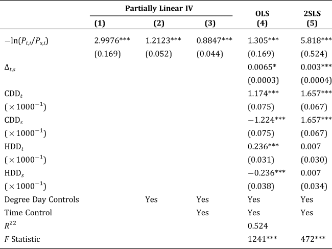
Additionally, all of the partially linear IV estimates are significantly different from the 2SLS results, which suggests that the 2SLS results are inconsistent. This may be because our controls and instrument have nonlinear effects on price and quantity, which cannot be captured by linear models. Specifically, we are likely to see temperature, which is proxied by CDDs and HDDs, to have nonlinear effects on electricity demand. The intuition here is that the amount of electricity needed to maintain room temperature varies nonlinearly with the outside temperature. So, using a linear functional form in the OLS and 2SLS regressions would produce inconsistent estimates. Alternatively, it may also be possible that the instrument, coal prices, affects electricity prices nonlinearly; this would also result in the 2SLS regression being inconsistent. On the other hand, the partially linear regression allows the control and instrumental variables to have nonlinear effects in both the supply and demand equation; this is shown equations 16 and 17. If the true functional form was linear for both the controls and instruments, we would expect the partially linear results to be closer to the 2SLS results. However, because the two types of regressions give significantly different results, the partially linear regression is more reliable since it is robust to nonlinearities that 2SLS cannot capture. So we believe that our third semiparametric fit, $\hat{\sigma } = 0.8847$ , is the most robust estimate of σ.
We also consider additional robustness checks for the estimate in fit (3). Firstly, we check if outliers are affecting the results meaningfully. We run the fit (3) regression but trim a larger number of outliers. We find that trimming an additional 1 percent, 5 percent, or 10 percent of outliers does not appear to significantly change the estimate of $\hat{\sigma }$ or meaningfully affect its standard error. Secondly, we test whether any particular states are driving the results. We run regression fit (3) on 48 subsamples; in each subsample, one of the 48 states in our data set is dropped out. We plot the results in the Appendix Figure B1. The mean and median of the estimates for σ are 0.8873 and 0.8860; additionally, 95 percent of the estimates lie in (0.8333, 0.9343). All of these estimates are highly significant—the average |t| value is 19.88, and the smallest |t| is 18.52. And although it seems that some of the estimates are (statistically) significantly from the full sample estimate of $\hat{\sigma } = 0.8847$
 (stdev = 0.044), the magnitude of the difference does not appear to be economically meaningful. That is, the largest estimate of $\hat{\sigma }$
 is 0.9793, which is only 0.0946 larger than the full sample estimate, while the smallest estimate is 0.8174, which is 0.0674 smaller than the full sample estimate. These differences are not meaningful in the practical application of our model.
Additionally, our estimates of σ appear to be much larger than estimates from the literature. Specifically, Schwarz et al. (Reference Schwarz, Taylor, Birmingham and Dardan2002) estimates σ to be between 0.02 and 0.04, while Herriges et al. (Reference Herriges, Baladi, Caves and Neenan1993) and King and Shatrawka (Reference King and Shatrawka1994) get estimates between 0.1 and 0.3. Our larger estimates may be due to limitations in our data—we use monthly data, while the literature uses hourly and daily data from real-time pricing experiments. However, in the following section, we implement our model numerically using our preferred estimate $\hat{\sigma } = 0.8847$ and then repeat our implementation using estimates closer to those in the literature. Our model's results do not change when using estimates from the literature; we discuss this in further detail in the “Robustness” section.
The Elasticity of Substitution between Renewable and Fossil Energy
So far, we have primarily focused on the (demand-side) intertemporal elasticity of substitution for electricity consumption σ. In this subsection, we discuss what implications σ has for the (supply-side) elasticity of substitution between energy inputs;Footnote 7 from here on, we will refer to this latter elasticity as e. Understanding this elasticity is important, because the substitutability of energy inputs determines the trade-offs required to transition into greener economy in the future. For instance, Acemoglu et al. (Reference Acemoglu, Aghion, Bursztyn and Hemous2012) provide a model where they argue: “When the two sectors [clean and dirty energy] are substitutable but not sufficiently so, preventing an environmental disaster requires a permanent policy intervention. Finally, when the two sectors are complementary, the only way to stave off a disaster is to stop long-run growth.”
The elasticity e is often assumed to be a constant value in the literature (Papageorgiou, Saarn, and Schulte Reference Papageorgiou, Saarn and Schulte2017). This is because existing models often represent the electricity sector using the production function

where $\tilde{Z}$ is the quantity of electricity output, $\tilde{X}_i$
 is the quantity of electricity-producing input, β i is a share parameter, and (ω − 1)−1 is the elasticity of substitution between the inputs. Since ω is a fixed parameter, the implied elasticity of substitution is constant. The literature often represents electricity production using a CES function and treats electricity as a single, homogeneous good. Furthermore, such models would generally have firms maximizing profit against a demand function based on some utility-maximizing agent. This approach captures the imperfect substitution between energy inputs in a tractable way. However, any results based on this model may be driven by the assumption that the elasticity of substitution between energy inputs, e, is constant.
Different from the exiting literature, our model implies that e is non-constant. We arrive at this conclusion through the numerical results which follow, although we can also see that e is non-constant in a simpler setting. Specifically, when σ = 1 and we have two periods and two technologies, the elasticity of substitution is given byFootnote 8

It is clear from the above equation that e will vary with the unit cost of the inputs c. However, what is not clear from this equation is the extent to which e varies with c or the link between intermittency and the elasticity σ. Since e does not have a tractable solution when σ ≠ 1, we parametrize and implement our model numerically.
To start, let technology 1 be coal power and technology 2 be solar power. These two technologies exemplify consistent fossil energy and intermittent renewable energy. Furthermore, let period t represent peak hours and period s represent off-peak hours. We assume that, holding prices equal, consumers prefer that approximately 60 percent of their energy arrive in period t and the remaining 40 percent arrive in period s; that is, we have α t = 0.6 and α s = 0.4. Since the union of both periods makes up only a single day, our model's assumption of an exogenous and constant ξ is fairly reasonable in this context.
Next, we normalize the remaining parameters in our model to a MWh basis rather than a per unit basis. This has no effect on the model at the theoretical level but makes it easier to empirically parametrize the unit cost of electricity production ${\vector c}$ . This is because the cost of electricity generation is generally reported in terms of $ per unit of electricity, while we originally set ${\vector c}$
 to represent cost per unit of input. Here, we set the cost parameters for each input equal to their LCOE ($/MWh).Footnote 9 In particular, we use estimates for 2023 for “Solar PV” and “Coal with 30 percent CCS” from Table 1b in EIA (2019b). Additionally, normalizing unit cost parameter ${\vector c}$
 requires us to normalize ξ as well; this ensures the rest of the model is unaffected. Consequently, ξrepresents the percent of total capacity utilized in each period; we assume coal uses 100 percent of its capacity in both periods, while solar can access 100 percent during peak hours and only 10 percent during the off-peak. In total, we have the following parameters.
Model Parameters:α t = 0.6, α s = 0.4, ξ 1 = (1, 1), ξ 2 = (1, 0.1), c 1 = 104.3, c 2 = 60.
We use these parameters with the theoretical results in the “Model” subsection of the “Electricity Market Equilibrium” section, to numerically compute the equilibrium. Specifically, given ξ and c, we can compute the equilibrium prices using the firm FOC p = ξ−1c (Equation 7). Then, knowing the prices, we can compute the price index given by the solution to the consumer's utility maximization problem $P = \sum _t\alpha _t^\sigma p_t^{1-\sigma }$ (Equation 4). Next, using the consumer's demand function $Z_t = \lpar {\alpha_t/p_t} \rpar ^\sigma \lpar {I/P} \rpar$
 , we are able to compute the solution for Z (Equation 3).Footnote 10 Finally, by definition, we have Z ≡ ξTX, which gives us the solution for X. In total, we have the equilibrium quantities X, Z and prices p.
Now, we explore how the elasticity of substitution e between these two technologies, solar and coal, changes with σ. Recall that for any two technologies i and j, the elasticity of substitution e i,j is given by:

We compute and plot our numerical estimates of e 1,2, the elasticity of substitution between solar and coal power, in Figure 1. To compute e 1,2, we numerically differentiate log (X 1/X 2) with respect to log (c 2/c 1). This is done by first computing the equilibrium quantities X across a range of cost vectors c; the results, in terms of log (X 1/X 2) and log (c 2/c 1), are shown in the first subplot of Figure 1. We only keep the results for X that correspond to interior solutions. Then, we numerically estimate e by computing the slope of log (X 1/X 2) with respect to log (c 2/c 1); this result is plotted in the lower subplot. Since log (X 1/X 2) is rising at an increasing rate with respect to log (c 2/c 1), we see that e is positive and increasing. We repeat this process with different values of σ, the IES in the consumer's utility function. Specifically, we use our estimate of $\hat{\sigma } = 0.8847\;\lpar {0.044} \rpar$ and its 95 percent confidence interval (0.7985, 0.9709). Overall, this shows how elasticity of substitution between solar and coal, e 1,2, changes with unit costs c and the consumer-side elasticity σ.

Figure 1. The Elasticity of Substitution between Solar and Coal
We see in Figure 1 that e 1,2 varies nonlinearly with the relative unit costs of each technology; in particular, it appears to take on a hockey stick shape. This shape can be understood as the interaction of two effects: intermittency and costs. The intermittency effect is that e falls when our electricity output is highly intermittent. The cost effect is that e is high when unit costs (c 1, c 2) differ significantly.
First, we explain the intermittency effect. Suppose that a majority of our energy came from solar; this corresponds to the left side of the graph where log (c 2/c 1) is lower and, as shown in the first subplot, log (X 1/X 2)is lower. In this case, a majority of the electricity is coming from an intermittent technology, therefore the overall supply of electricity is highly intermittent—it varies significantly over time. Specifically, solar generates primarily during peak hours, so consumers are being starved of electricity during the off-peak. This makes it difficult to replace even more coal power with solar. So the elasticity of substitution between solar and coal, e, is low. On the other hand, suppose that a majority of our electricity supply comes from coal; this corresponds to the right side of Figure 1. In this case, the electricity output is quite consistent over time. Consequently, replacing a marginal amount of coal input with solar input is not an issue. That is, making the overall energy output slightly more intermittent when it is already stable does not create as much disutility. Hence, when the intermittency of output is low, the elasticity e is relatively higher since it is easier to substitute between the energy inputs. In short, as the electricity output becomes less intermittent, e should rise.
Next, we study the effects of costs on e. We see quantities become more sensitive to unit costs when they differ significantly.Footnote 11 To understand why, suppose that the unit costs of two inputs are drastically different. And note that consumers want more electricity during peak hours compared to the off-peak based on the parametrization of α. This demand profile can only be achieved by combining solar and coal, since the electricity output of coal is constant, while solar produces more during peak hours. But if solar is extremely expensive, this makes it expensive to get relatively more electricity during peak hours than off-peak hours. Consequently, it may actually be more economical for consumers to rely primarily on coal. In other words, they would have to give up too much of their income to get more power during peak-hours than off-peak hours. Now, note that the elasticity e is defined as the derivative of the log difference in input quantities with respect to the log difference in unit costs. Consequently, when unit costs are very different, we would expect that small changes in costs would do much to change quantities, since costs (as opposed to other factors like intermittency) are primarily driving the market equilibrium. So ewould be high when log (c 2/c 1) takes extreme values. On the other hand, when unit costs are similar, the cost of generation does not matter for consumers as much as intermittency; so we would expect e to be low when log (c 2/c 1) takes more intermediate values.
We can add up the intermittency and cost effects to understand the shape of e. This means looking at three cases. The first case is the left-hand side of the second subplot of Figure 1, where solar is much cheaper. Here, the overall energy supply is highly intermittent, so e gets strongly pushed downwards; at the same time, the cost effect pushes e upwards. These two effects cancel out, and we see e take an intermediate value. The second case is near the middle of the subplot where we have more intermediate unit costs. Here, the intermittency effect moderately increases e, while the cost effect moderately decreases e. So, again, etakes an intermediate value. Finally, the third case is the right-hand side of the subplot where the majority of the electricity comes from coal. Both the intermittency and cost effect push e upwards. So, in this case, we see e being relatively high. In total, the two effects cause e to stay flat when the unit cost ratio, log (c 2/c 1), is low and then rise sharply when the unit cost ratio is high.
Additionally, these results and the intuition is not only limited to solar, as the following example illustrates. Consider a technology that produces most of its output during the off-peak period; this may be representative of wind energy. Now, for simplicity, suppose we parametrize this technology the same way as solar but with ξ 2 = (0.1, 1); this is simply the reverse of the parametrization we used for solar output per unit over time. Despite the fact that this technology primarily generates electricity in the lower demand period, the elasticity e between this hypothetical technology and coal as a function of the unit cost ratio will look nearly identical to that for solar in Figure 1.Footnote 12 This is because the intuition behind the cost effect and intermittency effect still applies. The intermittency effect causes e to rise as intermittency falls, and the cost effect creates a u shape. Like before, when we add these effects up, we get low e when we primarily rely on this new intermittent input and high e when we mainly rely on coal.
Secondly, we can see that the elasticity of substitution e 1,2 between solar and coal becomes larger as σ rises. To explain why, we first study the magnitude of e in two extreme cases: σ → 0 and σ → ∞. Specifically, we show that e will be small when σ → 0 and e will be large when σ → ∞. Understanding these two cases helps develop the intuition for why e rises with σ.
To start, consider the case where σ → ∞. Here, electricity consumption in each period is a perfect substitute for electricity consumption in other periods. Furthermore, from the equilibrium results, recall that the optimal solution was to only use whatever input had the highest cost-adjusted marginal utility $\sum _t\alpha _t\xi _{i\comma t}/c_i$ . This is because σ → ∞ causes utility becomes a linear function of electricity output in each period. So consumers only care about their total electricity consumption rather than when they get their electricity.Footnote 13 As a result, solutions generally turn into edge cases where we rely entirely on one input—whichever has the highest cost-adjusted marginal utility. Small changes in the cost of input i can cause it to become suboptimal. This means that the equilibrium quantity of the input may go from its maximum level to zero. Since e 12 = ∂log (X 1/X 2)/∂log (c 2/c 1) measures the sensitivity of the quantities of each input with respect to prices, we expect e to be extremely large in this case.
Next, consider the case where σ → 0. Here, electricity consumption across periods becomes complementary, with the optimal solution using some combination of inputs that make electricity as smooth as possible. This is because, when σ → 0, utility takes on a Leontiff functional form: $\mathop {\min }\limits_t \;Z_t/\alpha _t$ . In the context of our parametrization, this would imply that consumers want a relatively fixed ratio of peak and off-peak consumption. We know that coal offers a strictly smooth output, while solar offers more during peak hours. Hence, the equilibrium would be one which primarily uses coal and then a small amount of solar to account for the fact that consumers demand slightly more electricity during peak hours. Furthermore, even if unit costs change, the optimal solution would still require the consumer to maintain a relatively fixed ratio of peak and off-peak electricity cosnumption to maximize utility; this then requires maintaining a fixed ratio of solar and coal. Consequently, changes in the unit cost of solar and coal would do little to affect the equilibrium ratio of inputs. Thus, since e measures how sensitive the two inputs are with respect to their unit costs, it would be close to zero in this case.
These two extreme cases illustrate the link between e andσ. When σ rises, consumers care less about smoother consumption. Consequently, consumers are more willing to accept intermittency in the electricity supply. This causes the implicit demand for inputs to become relatively less sensitive to intermittency and relatively more sensitive to their costs. As a result, the substitutability of intermittent and consistent technologies rises, so we see e increase.
Thirdly, we can see that the higher levels of σ cause e to change shape. To understand why, we can appeal to the intermittency effect and the cost effect. Note that σ rising makes intermittency matter less; this diminishes the intermittency effect. As a result, we see the cost effect dominate. Recall that the cost effect creates a u-shape, while the intermittency effect is what causes e to fall when we rely heavily on solar. Now note how when σ rises, e becomes more u-shaped.Footnote 14 This is because the intermittency effect becomes more diminished and the cost effect takes over. By this logic, if we keep raising σ, the level of e becomes increasingly larger; at the same time, we would also see it become more u-shaped as the cost effect takes over.
To summarize, e depends on two factors, cost and intermittency, while σ affects the importance of intermittency. When costs are highly different, e rises—this is the cost effect. When the output of electricity is highly intermittent, e falls—this is the intermittency effect. These two effects combine to give e the shape we see in Figure 1. Furthermore, at higher levels of σ, consumers care less about smoother electricity consumption and thus intermittency matters less. So higher σ diminishes the magnitude of the intermittency effect resulting in a larger e. Additionally, a smaller intermittency effect causes e to take on more of a u-shape as the cost effect dominates. Overall, these numerical results for e are consistent with the analytic results and intuition from earlier.
Environmental and Energy Policy Implications
A simple but important finding here is that e, the elasticity of substitution between renewable and fossil energy, is not constant. Furthermore, it appears to fall with the level of intermittency. What implications does this result have?
Revisiting Past Models
To start, we consider how a variable elasticity of substitution affects past models of the energy sector. As an example, consider the results of Acemoglu et al. (Reference Acemoglu, Aghion, Bursztyn and Hemous2012). Firstly, they find that the short-run cost of policy intervention is increasing with the elasticity of substitution between clean and dirty technologies.Footnote 15 Additionally, their article states that the cost of delaying intervention is increasing with the elasticity of substitution. Secondly, Acemoglu et al. argue that, when the discount rate and elasticity of substitution between clean and dirty energy (e) is sufficiently low, a disaster cannot be avoided under laissez-faire.Footnote 16 And, finally, Acemoglu et al. find that, “when the elasticity of substitution is high … a relatively small carbon tax is sufficient to redirect R&D towards clean technologies.”
Based on our results, each of these statements has a complementary interpretation in terms of intermittency. For instance, the first statement suggests that the cost of policy intervention is decreasing with the intermittency of clean technologies; the cost of delaying intervention is decreasing with intermittency as well. This is because the elasticity of substitution between renewables and fossil fuels becomes small when renewables are more intermittent. So in other words, delaying policy intervention will be the most costly in regions with access to clean, non-intermittent energy (such as hydro and geothermal energy). Secondly, when the discount rate is sufficiently low and the intermittency of clean energy is sufficiently high, a disaster cannot be avoided under laissez-faire. The intuition here is that, even if clean energy became relatively cheap, its intermittency would prevent it from adequately substituting for fossil energy. Finally, Acemoglu et al. argue that the size of a carbon tax should be inversely proportional to the elasticity of substitution and should decrease over time. Recall that, in our model, the elasticity of substitution e changes with relative prices; when fossil fuels are relatively cheap, e is large. Hence, this implies we need a relatively small carbon tax early on to spur research. As technological change makes renewables cheaper, fossil fuels will become relatively more expensive so e will fall; thus, the carbon tax will need to increase over time. These dynamics (a rising carbon tax) contrast with the results of Acemoglu et al., who numerically show that an optimal carbon tax should decrease over time when e is sufficiently large. A potential resolution to these contradictory solutions may be to take an intermediate route and maintain a constant carbon tax over time.
Carbon Taxes and Their Distributive Consequences
Our results also suggest that carbon taxes can have important distributional consequences. Earlier, we showed that the elasticity of substitution between renewable and fossil fuels (e) is non-constant and falls with the intermittency of present generation. This further implies that the elasticity of demand for generation technologies is non-constant as well. Specifically, the elasticity of demand for non-intermittent energy increases and then decreases with respect to its own price. Using the earlier numerical example of solar and coal power, we show this explicitly in Figure 2. As the price of coal power rises significantly beyond its current price, demand gets more elastic because its price becomes the primary factor disincentivizing its use. But initially, a rise in the cost of coal power causes its demand to become inelastic. This is because a rise in the price of coal shifts generation towards solar; consequently, generation becomes more intermittent and demand for coal becomes less price-sensitive since it is needed to help smooth electricity generation. This relationship should be of concern for policy makers considering a pollution tax. Consumers in regions without access to clean, non-intermittent energy will have the most inelastic demand for fossil fuels; hence, they will bear the greatest welfare losses from a tax on pollution/carbon. On the other hand, consumers in regions that have access to dispatchable, renewable energy such as hydropower will see smaller welfare losses; the demand for fossil fuels in these regions will not be as inelastic, because dirty generation can be replaced with non-intermittent, clean generation. All in all, if a carbon tax were implemented federally and its revenue were distributed equally, it may nevertheless function as an inequitable, between-state welfare transfer due to differences in the availability of renewable energy technology. This same argument would apply to carbon quotas.
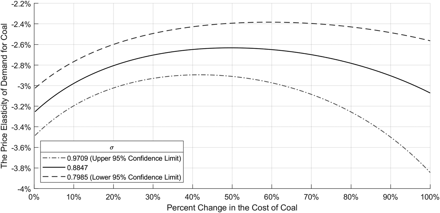
Figure 2. The Price Elasticity of Demand for Coal Power
The Case for Subsidizing Battery Research
However, there are alternative policies that can mitigate this distributional side effect. One such policy is a research subsidy for improving battery technologies. Reducing battery costs, improving their storage capacity, and reducing their energy loss can allow intermittent renewables to far more easily substitute for traditional, fossil energy. To understand the magnitude of this effect, we again provide a numerical example using solar and coal. We aim to understand how batteries effect substitutability, so we consider a parsimonious model where batteries are used to shift a portion of solar energy output from its high-output period to its low-output period.Footnote 17 Specifically, we initially parametrized solar with ξ 2 = (1, 0.1), implying that it functions at 100 percent of its potential capacity during the peak and at 10 percent of its potential capacity during the off-peak; this is far from matching consumer demand. So we represent solar output with batteries using ξ 2 = (0.95, 0.15) and ξ 2 = (0.90, 0.20); this is equivalent to transferring 5 percent and 10 percent of solar output. We plot our results in Figure 3. It is immediately clear that making solar output more consistent through the day results in a large increase in the elasticity of substitution e 1,2. Moreover, e 1,2 no longer tapers off around 4 as solar becomes the dominant source of electricity. Rather, with batteries, cost plays a much larger role in determining the optimal quantity of each technology even when solar is relatively cheap. Overall, shifting even a small fraction of solar output using batteries can significantly improve solar power's substitutability with coal.
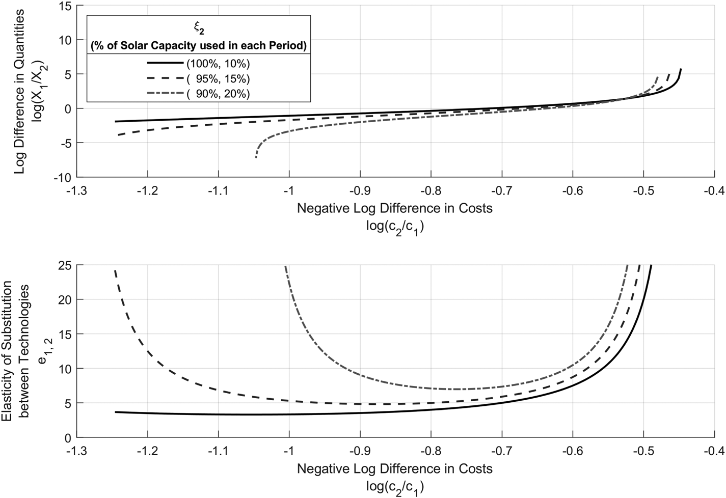
Figure 3. The Effect of Battery Storage on the Elasticity of Substitution between Solar and Coal
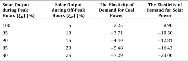
Consequently, batteries can complement reductions in the cost of intermittent renewables and mitigate the distributional side effects of a carbon tax. As shown in Figure 3 the elasticity of substitution between solar and coal rises significantly as solar becomes less intermittent; this implies that a change in the relative price of solar would have a far greater effect on solar adoption if batteries were employed with solar. Hence, if policy makers aim to promote the use of renewables, they should subsidize research that reduces the cost of renewables as well as research that improves battery technology. Using both policy instruments can be more effective than either alone. Additionally, the second benefit of batteries is that they mitigate the distributional problems of a carbon tax. This is because, by reducing the intermittency of renewables, batteries make demand for fossil fuels less inelastic. We specifically show this elasticity would change with another numerical example in Table 3; as in Figure 3, we model batteries that shift solar output towards the off-peak. We then estimate the elasticity of demand for coal power around its initial price; this elasticity is decreasing at an increasing rate with the percent shift in solar output. The practical implications of this are straightforward. Researching and implementing battery technology can reduce the welfare losses from a carbon tax. Moreover, regions without clean, consistent renewables would benefit in particular, because they will be able to combine intermittent technologies with better energy storage to help transition away from fossil fuel energy. In short, subsidizing battery research can reduce some of the unintended distributional consequences of carbon taxes while mitigating environmental damage.
Table 3. The Effect of Battery Storage on the Elasticity of Demand
Learning-by-Doing and Intermittency
Learning-by-doing, originally introduced by Arrow (Reference Arrow1992), refers to an increase in productivity or quality as firms acquire experience producing a particular good. In the context of renewable policy, a common argument is that knowledge from learning-by-doing spills over across firms, and thus governments should subsidize renewable adoption (Borenstein Reference Borenstein2012).
Our results suggest that renewable subsidies aimed at correcting the positive externalities of learning-by-doing should vary geographically. This is because our model shows that the substitutability of renewable energy depends on their intermittency and the preexisting technologies used for generation in a particular area. And both intermittency and existing technologies vary by region; for instance, the intermittency of wind power may vary due to regional differences in climate. Consequently, the level of subsidies needed to promote the deployment of renewables can vary geographically.
But are geographic differences in substitutability economically significant? As an example, consider equivalent solar panels deployed in two different regions. In the first region, the solar panels generate energy at 100 percent of their capacity during peak hours and at 10 percent during the off-peak; on the other hand, in the second region, the same solar panels produce at 90 percent during the peak and 20 percent during the off-peak due to geographic differences. This is similar to the earlier exercise where we studied how substitutability would change if we shifted a portion of solar output toward the off-peak using batteries. Specifically, we can see how the elasticity of substitution differs between the “(100 percent, 10 percent)” region and “(90 percent, 20 percent)” region using Figure 3. That is, if the regions are otherwise equivalent, solar is far more substitutable for fossil energy in the (90 percent, 20 percent) region due to its slightly smoother output profile. Specifically, at the prices used for the numerical simulation earlier (c coal = 104.3, c solar = 60), the point elasticity of demand for solar power is −8.9 in the (100 percent, 10 percent) region and 12.8 in the (90 percent, 20 percent) region; this is given in Table 3. Consequently, the level of subsidies needed to promote solar adoption in the former region would need to be about 43 percent larger than those in the latter region due to differences in intermittency.
Along with geographic variance in intermittency, preexisting generation technologies also vary by region and can create large differences in substitutability between alternative power generation feedstocks. For instance, consider two regions where the first primarily uses natural gas and the latter uses coal power. It is easier to promote the adoption of intermittent renewable energy like solar in the first region, since the output of electricity from a natural gas plant can be deliberately changed within an hour. Again, the intuition is similar to that from the battery storage example where smoothing solar output increased its substitutability. In this case, solar and natural gas are strong substitutes, since natural gas can fill gaps in solar's intermittent generation; the same idea would apply to other intermittent renewables such as wind. On the other hand, coal is a base load technology that is much less flexible in its intra-daily output. So, in the region relying on coal power, increasing the share of solar power would necessarily create greater intermittency in the overall electricity supply. This means solar and coal are much weaker substitutes than solar and natural gas. More generally, the elasticity of substitution between intermittent renewables and fossil energy varies significantly based on type of fossil energy in question. This variation in substitutability creates differences in the efficacy of subsidies/taxes aimed at promoting renewable adoption. Therefore, regional differences in the preexisting technologies used for generation can be economically significant and should be accounted for when designing energy policy aimed at correcting externalities from learning-by-doing.
Adjusting Future Models
Given that traditional assumption of a CES relationship between renewable and fossil energy appears to be inaccurate, we offer two alternative approaches for future models. The first approach is to directly integrate our model within a given framework. The second approach is to assume a variable elasticity of substitution (VES) structureFootnote 18 between clean and dirty energy. These two approaches have their own advantages/disadvantages and serve different purposes.
Direct Integration: The first approach is better suited for numerical models. For example, our model of the energy sector can be embedded within a Computational General Equilibrium (CGE) model. CGEs, specifically ones designed to study energy and environmental policy, tend to assume a CES relationship between generation technologies and treat electricity as a homogeneous good. On the other hand, our representation of the energy sector directly models the source of imperfect substitutability between generation technologies—intermittency. Consequently, embedding our model within a CGE would improve its predictive accuracy by giving it more realistic microfoundations.
Furthermore, implementation can be done with relatively few modifications to standard CGE. To start, CGEs already use CES utility to model consumer preferences. In order to integrate our method of modeling electricity consumption, a CGE practitioner need only to rewrite preferences as:

where the intertemporal elasticity of substitution for electricity consumption is given by σ = 1/(1 − ϕ), the elasticity of substitution between all consumer goods is given by 1/(1 − η), the consumption of each good is given by Z i, and the consumption of electricity in each period t is given by Z elc,t. This can be simplified to:


where Z elc is an aggregate electricity good. Next, we consider the production functions for electricity production in each period. These are simply linear, since the total electricity produced in a period is equal to the sum of electricity produced by each technology in that period. That is, we have

where X i is a generation technology and ξ i,t is its output in period t. The parameters for ξ 1,t must be estimated using additional data. For fossil fuels, ξ i can remain constant over time. For intermittent renewables, ξ i,t may be set to empirical estimates of the average output per unit of X i in period t.Footnote 19 Additionally, the supply-side equations for building capacity in each technology can be modeled using the usual CGE approach; total cost is given by the sum of costs for each input factor, and total quantity is given by a CES of the input factors used to build capacity (X i). Finally, since these functional forms are equivalentFootnote 20 to those used in standard CGEs, they can be calibrated using the usual procedures and a social accounting matrix. So overall, implementing our model within a CGE can be done in a fairly simple way.
VES Approximation: The second approach is to use a variable elasticity of substitution function to model the relationship between clean and dirty energy. A VES function would approximately capture the dynamics of e, the elasticity of substitution between clean and dirty technology while keeping a theoretical model relatively simple. The latter is because assuming a VES structure between clean and dirty energy only requires considering one more parameter than a traditional CES function. To be more precise, the VES function is defined in Revankar (Reference Revankar1971) as


where ω, δ, ρ, and γ are parameters, Z is the output, X 1 and X 2 are the inputs, and e is the elasticity of substitution between X 1 and X 2. In the context of an electricity sector, we can think of Z as electricity output, while X 1 and X 2 represent dirty and clean inputs. Note that e is a linear function of X 1/X 2; this relationship allows a VES function to approximate the effects of intermittency. To show why, we plot e against its VES approximation $\hat{e}$ for solar and coal in Figure 4. This approximation was fit by running OLS against the numerical results for e while holding the intercept fixed at 1.Footnote 21 We can see that, as either the capacity of solar or coal dominates the market, the approximation becomes weaker. But overall it seems to mimic the shape of the true elasticity of substitution e implied by our model of intermittency. Hence, a VES function is a reasonable alternative to a CES function—it better models intermittency while also maintaining parsimony.

Figure 4. The VES Approximation of the Elasticity of Substitution between Solar and Coal
One potential objection to using the VES function is that it assumes the elasticity of substitution e approaches 1 when the majority of electricity output comes from renewables (X 1/X 2 → 0). And a VES structure assumes linear e, which does not seem to be the case in Figure 4. However, both these assumptions may still be fairly reasonable in the right context. That is, suppose renewable energy was highly intermittent and that the consumer's elasticity of substitution σ = 1. Firstly, this results in renewable and fossil energy entering a Cobb-Douglas relationship (e = 1) as X 1/X 2 → 0, which supports the VES assumption of an intercept of 1. Secondly, no matter the relative prices, whenever the renewable technology is highly intermittent, e becomes perfectly linear with respect to X 1/X 2; this supports the VES assumption of linearity. The proofs for both are given in Appendix A.C. Hence, in these cases, a VES approximation can perfectly match e. Additionally, even when the consumer's elasticity of substitution is not 1, e may still be approximately linear; this is shown in Figure B4 where we consider our estimated $\hat{\sigma } = 0.8847$ . In short, the assumptions made by a VES structure may nevertheless be accurate in certain cases.
Overall, using a VES function is a reasonable alternative to directly modeling intermittency. It allows theorists to derive policy implications from intermittency without relying too heavily on numerical models. Furthermore, it keeps theory simple, since the elasticity of substitution can be represented as a linear function of a single parameter β. And this parameter can be estimated econometrically, so theoretical models assuming a VES structure can offer empirically based results. Finally, it may even be of use for CGE modelers. Its structure is simple enough to be calibrated with a given set of data, while its implementation can produce simple but reasonably accurate models of energy sectors with intermittency.
Robustness
As a robustness check, we reproduce the estimates of e shown in Figure 1 across a larger range of values for σ. This allows us to evaluate the extent to which our results for e are driven by our estimate of σ. Specifically, we consider parametrizations of σ closer to estimates from the literature. Herriges et al. (Reference Herriges, Baladi, Caves and Neenan1993) and King and Shatrawka (Reference King and Shatrawka1994) estimated σ to be between 0.1 and 0.3, while estimates by Schwarz et al. (Reference Schwarz, Taylor, Birmingham and Dardan2002) were between 0.02 and 0.04. Additionally, we consider σ = 1 and σ = 2, which is closer to our OLS and 2SLS estimates. We estimate e using values of σ around these values and plot our results in Figure 5.
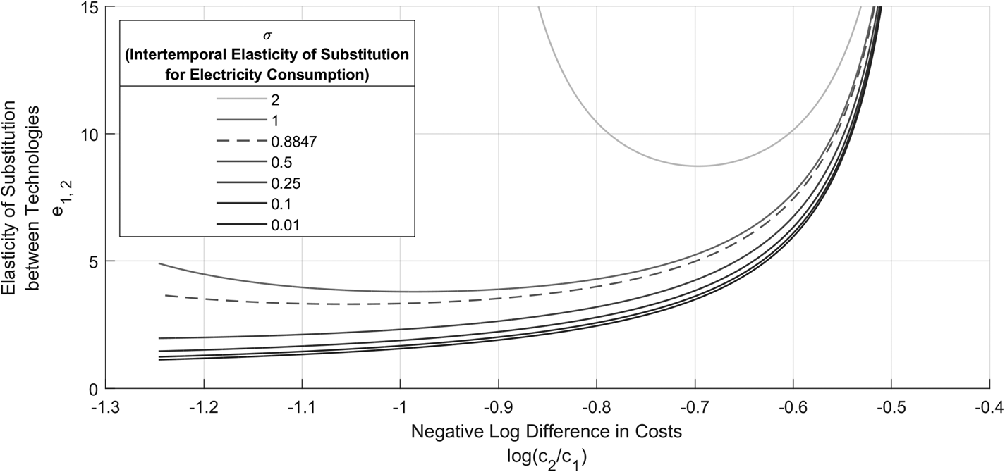
Figure 5. The Elasticity of Substitution Between Solar and Coal (Robustness Check)
Using values of σ closer to our OLS and 2SLS estimates causes e to be much higher. This is because the OLS and 2SLS results have σ higher than our partially linear specification. This suggests that intermittency is much less of a problem for substitutability if we parametrize our model using the 2SLS results. However, as argued in the “Results” section, the partially linear model is robust to functional form misspecifications and nonlinearities, while 2SLS is not.
When using the literature's estimates of σ, which are much lower than ours, we find lower values of e. The estimate for e near the parametrized value of c is 10.29 when σ = 0.8847 (our estimate) and 8.93 when σ = 0.1. Furthermore, the difference between the implied elasticity e when σ = 0.1 and when σ = 0.01 is fairly small. Furthermore, the difference between the results implied by our estimate of σ and that of the literature gets bigger when solar is relatively cheaper (left-hand side of the plot); this is because of the intermittency effect, as discussed earlier.
Although these differences from using the literature's estimates appear to be large, they do not negatively affect the implications of our results. Thus far, we have discussed how intermittency complicates environmental policy. The literature's estimates of σ are lower than our own; in other words, the literature finds that consumers care strongly about smoothing their electricity consumption. Consequently, if one puts more weight on the literature's estimates, then intermittency is more important than we have argued with our results. That is, when σ is lower, it is harder to substitute between intermittent renewable and reliable fossil energy; this is shown in Figure 5, where e is lower at all relative prices log (c 2/c 1). As a result, using the literature's estimates of σ makes the distributional consequences of energy policy more pronounced and research into batteries more important. Hence, the policy implications from our article are strengthened when using the literature's estimates of σ.
Conclusion
In this article, we have offered a framework for understanding the economics of intermittent renewable energy that bears in mind the critique offered by Joskow (Reference Joskow2011). That is, our model evaluates the economic value of a generation technology by integrating its production profile with the market value of electricity. Moreover, consumers in our model treat electricity as a heterogeneous good differentiated by time. The empirical parametrization of our model and its numerical results suggest that the elasticity of substitution between renewable and fossil energy is non-constant. We have shown that this has important implications for policy and future models.
With respect to policy, we have shown (i) the welfare effects of carbon taxes and renewable subsidies depend on the intermittency of renewables and thus vary geographically; (ii) the effect that renewable subsidies have on promoting the adoption of renewables varies geographically; (iii) the combination of (i) and (ii) can create a trade-off between efficiently and equitably preventing climate change; (iv) subsidizing battery research can complement other policies by increasing the substitutability of renewable and fossil energy; (v) improving batteries can mitigate the unintentional distributional consequences of carbon taxes and research subsidies. Additionally, we have qualitatively evaluated the results of Acemoglu et al. (Reference Acemoglu, Aghion, Bursztyn and Hemous2012) in a setting where renewables and fossil fuels have a nonlinear elasticity of substitution. Based on their framework, we have further argued that: (vi) the short-run cost of policy intervention is decreasing with intermittency; (vii) the cost of delaying intervention is decreasing with intermittency; (viii) when the discount rate is sufficiently low and the intermittency of renewables is sufficiently high, a laissez-faire equilibrium would require policy intervention to prevent disaster; (ix) when renewables are moderately intermittent, an optimal carbon tax should remain approximately constant over time.
Table 4. Parameter Restrictions for Z, X > 0
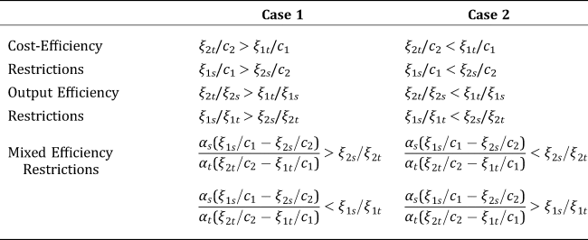
Notes: The inequalities in this table assume that all elements of ξ are greater than 0. The full proof given below provides equivalent restrictions for the zero cases.
Given how strongly the elasticity of substitution between renewable and fossil energy varies with relative price, future models of intermittency should not assume a CES structure. This work showed that to integrate the proposed framework with a numerical model, such as a CGE, may improve predictive accuracy by providing more realistic microfoundations. On the other hand, theoretical models would be better served by a more analytically tractable alternative. Therefore, we suggest theoretical models use a VES production function to approximate the effect of intermittency on the elasticity of substitution between renewable and fossil energy. Under certain conditions, our own model simplifies to a VES case; hence, the VES production function can reasonably approximate for our full model in a more tractable way.
While constructing our model, we made several simplifications for tractability. For instance, we set aside modeling reliability—stochastic or otherwise unpredictable variation in output. An aim for future research may be to develop a model of clean and dirty energy that incorporates both intermittency and reliability in a multi-period setting. This could involve integrating our framework with that of Helm and Mier (Reference Helm and Mier2019). Additionally, another avenue for future research may be to explicitly model the effects of battery technology and how storage interacts with intermittency and reliability. Such models can offer more accurate predictions/suggestions for policy makers and bring theory closer to reality.
Supplementary material
The supplementary material for this article can be found at https://doi.org/10.1017/age.2020.7.
Acknowledgments
This work was supported by the Northeast Sun Grant #5701-RU-SDSU-G640. We would also like to thank Prof. Roger Klein and the participants of the NAREA 2019 Workshop for helpful comments.


 Open access