This sessional meeting discussion relates to the paper presented by Tim Berry and James Sharpe at the IFoA sessional webinar held on 5 July 2021. The Moderator (Mr A. D. Smith, Hon F.I.A): Good afternoon, everybody, and welcome to this sessional meeting on “Asset Liability Modelling in the Quantum Era.” My name is Andrew Smith and I teach Actuarial Science at the University College Dublin. Welcome especially to those of you who are dialling in from overseas.
We have two speakers today: Tim Berry and James Sharpe. Tim is a consulting actuary. He specialises in valuation and pricing models in life insurance, primarily in reinsurance. Tim’s real strength is in creating insightful, user-friendly and efficient models. He has worked in Hong Kong and Tokyo for many years. He is now back in the UK, but still has a good portfolio of international clients. He regularly chairs actuarial learning events and has an amateur interest in physics and hiking in warm places, which today probably includes London.
James Sharpe is also a consulting actuary. He has more than twenty years of actuarial experience, and recently he has done a lot of work on calibrating internal models on matching adjustment portfolios and asset liability matching. He chairs the IFoA’s Extreme Events Working Party, of which I also happen to be a member.
So without further ado, I am going to hand over to Tim (Berry) and James (Sharpe) to present to us on the topic of “Asset Liability Modelling in the Quantum Era.”
Mr J. A. Sharpe, F.I.A. (introducing the paper): There are six items on the agenda. For the first item, “Introduction – What is Asset Liability Modelling (ALM)?”, we talk through what this means and the general principles used under ALM. The second section is on “Specification of the ALM Problem” and specifying what we are trying to do in ALM. In section three, we look at “Early Attempts to Solve the ALM Problem,” examining how actuaries have been looking at this problem for the last 300 to 400 years and how the approach has evolved over the years into what people do today. The fourth section on “Current Solutions to the ALM Problem” covers the solutions we see in insurance companies operating in the UK, Europe and the US today. Section five, which forms the majority of this presentation, is on “Quantum Computing” and how this can be used to solve the ALM problem. Section six contains our conclusions.
So, what is ALM? To address this, we took a set of points first described by Arthur Bailey in his paper from 1862. We liked these points because they were relevant at the time, but remain relevant today, 160 years later. Arthur Bailey’s paper was the first articulation of efforts to deal with the ALM problem. The first point that Mr Bailey came up with is the consideration of default risk. A primary consideration is to minimise default risk for assets that we are considering for backing our liabilities.
The second point Mr Bailey came up with is that we would prefer a higher yield to a lower yield. So, provided we have controlled our default risk and have a good understanding of this, a higher-yielding asset is preferred to a lower-yielding asset, for the same security of capital.
The third point Mr Bailey came up with was that some of the assets should be readily convertible or liquid. If we only have illiquid assets, then this can create problems due to changes in liabilities or short-term claims/outgoings.
The fourth point raised was the concept of a liquidity premium, which is still very much around today, where illiquid assets typically would have higher-yielding returns than assets that are more liquid but of the same security/default risk. Even in 1862 people were looking for the same type of liquidity premium that continues to be sought out today, to back the long-term liabilities. Finally, the fifth point, which perhaps is not so common today, is that capital should be employed to aid the life assurance business itself.
The above principles were a clear articulation of the key underpinnings of ALM and what an insurer might try to do when selecting assets to back long-term liabilities.
We now proceed to the section dealing with the specification of the ALM problem. We try to minimise the value of the assets to back our liabilities, subject to several constraints. Minimising the market value of the assets is the same as maximising the yield on those assets. The constraints we have noted are typically what you would expect under regulatory requirements or similar to those that the management of an insurance company might be focused on. These would be items like minimum security requirements. For example, with a matching adjustment portfolio, there is a limit on BBB rated assets where you can have a “matching adjustment” (MA) higher than a BBB asset.
Insurance companies themselves might also have specific limitations on assets of a particular credit rating. For example, not all investments need to be allocated in BBB or above assets. It may be possible to invest in assets with other ratings as well. There could also be a maximum exposure to interest rate risk to limit the impact of interest rate movements, and similarly for inflation or currency risks. There could also be a requirement to maintain a minimum level of liquid assets, such as gilts or cash, so that you can meet your liquidity requirements. The minimum present value of asset cash flows compared to liability cash flows is also a requirement on the MA portfolio, as well as other requirements. These include a minimum cash flow mismatch in any given year, so that over any year during the term of the liabilities there is not a large deficit which might need to be subsidised by a large surplus in another year. Lastly, there may also be some constraints to minimise capital requirements, for example regulatory or risk capital requirements.
The next section outlines a brief history of ALM that prepares us for the discussion about quantum computing. There is a quote from Charles Coutts in 1933 where Mr Coutts, who was the President of the Institute of Actuaries, said “An attempt should be made to ‘marry’ the liabilities and the assets as far as possible.” This was picked up in a book by Craig Turnbull entitled “A History of British Actuarial Thought,” pointing out that no quantitative method had been introduced in ALM until 1933. For over 70 years it had still been looking at qualitative points and principles rather than mathematical calculations. But the move to quantitative methods happened in 1938 with the Macaulay Duration. In principle, if the asset time-weighted average of cash flows was matched with that of the liability time-weighted average of cash flows you could argue that the asset and liability positions were matched. Items like changes in interest rates could be minimised by having a closely matched time weighted average of your cash flow, that is by matching the duration. It was not until the 1950s that this matching of durations was formalised, and that was done so by Frank Redington in his immunisation formula. It is a very well-known formula used by many actuaries to this day.
Looking at Redington’s immunisation formula, the value of liabilities is set equal to the value of assets. Any asset amounts above this are not subject to this method and are considered outside this framework. Then, looking at the present value of the asset and liability proceeds, the portfolio is de-sensitised to small changes in interest rates. This means that if interest rates move, we want to ensure the surplus (amount of assets over liabilities) is not negatively reduced. The way Mr Redington did this was to use Taylor’s approximation for a small change in interest rates. A change in the value of assets with respect to interest rates, minus the change of value of liabilities with respect to interest rates, can be approximated to by Taylor’s theory. Redington concludes that if you set the first derivatives (in the Taylor series) to zero and the second derivative to greater than zero, then in cases of a small interest rate change, you would make a small profit/observe a small increase in your surplus subject to small changes in interest rates such that none of the higher order terms impacts (in the Taylor series expansion) surpasses the impacts of the first two derivatives. This is quite a simple method, but also very effective.
In Redington’s paper, he talks about immunisation with respect to interest rates, but it could also be applied to other risks such as inflation or currency risk. Redington notes that there are infinitely many solutions to his immunised equation, but he does not comment as to which solutions might be preferable, such as maximising yield whilst minimising credit risk. You are still left with this combination of quantitative methods in unison with Bailey’s qualitative descriptions from 1862. Furthermore, if we are choosing solutions based on single present values, it is possible to have cash flow mismatches in particular years that could cause liquidity issues. Those problems are there because people did not have the computing power they now have. Following a 20-year period after the World War II, we did see huge progress in computing power, which led to new solutions and the first introduction to operations research methods. There was a huge level of research during the World War II on operations research methods, where computers were used in places like Bletchley Park. At the end of the war, the people who worked in the field produced a lot of papers that went out into industry, including insurance companies. In principle, operations research is all about maximising or minimising certain parameters subject to a number of constraints. This is an ideal set of tools for the ALM problem we have talked about where we are minimising the market value of the assets subject to a list of constraints. The simplest algorithm you might use is to consider all possible combinations of assets and see which gives you the best value(s). If you use a non-quantum computer to do this, it might take a significant amount of time. For example, if you have 100 assets, you get 2100 possible combinations of those assets and that is only if you consider the possibility of investing 100% in each asset, and not considering partial holdings, for example, 50% of one asset and 50% of another, which would mean many more combinations. 2100 is approximately equivalent to 1030 possible combinations.
Whilst that is an algorithm that could be written, it cannot be solved within a tangible timeframe. These operations research techniques are all about identifying algorithms that can reduce that timeframe by narrowing down the number of scenarios you look at. This is done by dismissing a large number of scenarios from the outset. Using these methods, large pensions or insurance company portfolios might only take a few minutes to run.
There are two key parts of an operations research type problem you need in order to find a solution to the ALM problem is. The first is to identify and define the problem in mathematical terms, and that can often be visualised in n-dimensional spaces. In our example we use two assets and try to look at the optimism proportion of these two assets, which would maximise a return subject to a number of constraints. If you had 500 assets, it would be a 500-dimensional shape. There is a whole host of possible algorithms you could use depending on whether the problem is linear or non-linear. Once you define the shape and specify the problem, then you would apply this algorithm and it would find what you hope is the maximum. It either is the maximum or, if it is a non-linear problem, it might be only close to the maximum.
This is a description of the current ALM practices that insurance companies are using. As mentioned previously, such an algorithm might take several minutes to run and you can effectively solve this problem. It just narrows down the number of possible solutions it looks at and that means it goes from taking an impractical amount of time, by considering all possible combinations, to taking five or ten minutes. It is quite an efficient process, but if you are a large insurance company, you might want to run 500,000 scenarios on your portfolio. If you wanted to optimise in every one of those scenarios, taking 10 minutes to do each of these optimisations would still be an unworkable amount of time. In order to resolve this problem, we need to look at alternative approaches. The next step that is being considered is quantum computing, where timeframes are vastly smaller for these kinds of problems. So, to talk us through that next stage, I will hand over to Tim (Berry).
Mr Tim Y. Berry, F.I.A.: Before we consider how a quantum computer can solve the ALM problem, we will first consider some of the properties of quantum mechanics that are relevant to quantum computers.
The Copenhagen interpretation of quantum mechanics was devised in the 1920s by Bohr and Heisenberg. In this research, microscopic quantum objects were deemed to not have definite properties prior to being measured. The wave function is a mathematical representation of the system, and from this you can define probabilities of the measurement results. When you measure the objects, the wave function collapses and becomes certain in properties. In our illustration, we show a photon on a plane, and the vertical axis is the probability of where it might be. When you look at it, it collapses into a particular place, but before you looked at it, it had a range of probabilities.
The two key features of quantum mechanics are “superposition” and “entanglement.” To get an idea about superposition, we show an experiment in our diagrams where you create a photon at the source and send it towards a partially reflective mirror where there is a 50% chance it could go into box A or a 50% chance it could go into box B. Each of the boxes has a slit, which are opened simultaneously, through which the photon then leaves the box and heads towards a screen where it is measured as a dot. If the experiment is repeated many times, one photon at a time, then an interference pattern appears on the screen. The results of the pattern shown indicate that each photon was originally in both boxes at the same time. This principle of the photon being in two positions at the same time is an example of superposition.
The other key property of quantum mechanics is “entanglement.” Imagine if you create two electrons in such a way that they have opposite spin properties, so if the first electron is an “up” electron, then the other electron is a “down” electron. Imagine that you create two electrons (one with an “up” spin and another with a “down” spin) and put them in separate boxes, and then keep one box and send the other box to the other side of our galaxy. If we open the box in front of you and you discover it is an “up” electron, then you know that the other electron must be a “down” electron. What is surprising about this is that before you looked at that electron, it was in its superposition state of being “up” and “down.” By looking at it, it became an “up” electron which means you have made something else at the other side of the galaxy change into a “down” electron. This was obviously unexpected and led to the EPR (Einstein-Podolsky-Rosen) paradox in the 1930s, which described this as “spooky action at a distance” and suggested that the wave function is not how reality is. In the 1960s, John Bell formulated the “Bell theorem,” which was later tested and validated in the 1970s. Although this experiment has been tested to a very high degree of accuracy, what is still not fully understood is what is occurring at the collapse of the wave function. Whilst the Copenhagen interpretation is the most widely accepted interpretation, there are others too, most noticeably the many-worlds theory, where instead of the wave function collapsing, a parallel universe might emerge at that time.
Next, we move onto some ideas behind quantum computing. Quantum computers have quantum bits or qubits, and these can be compared to classical bits. A classical bit, in a classical computer, can take a value of zero or one, whereas the quantum bit can be in a superposition state of both. It is both zero and one, until it is measured, and its wave function collapses, and then it becomes either one or zero. Using entanglement, it is possible to create a set of connected qubits. If we consider three bits, then there are 23 possible combinations. A classical computer might perform a calculation on each combination sequentially, whereas quantum computers can use and calculate all the states at once. If this example was extended to 1,000 bits then a classical computer would not be able to manage this. In reality, quantum computing is more complicated and, for example, if you were to look at the qubits, you would imagine it would collapse into one of the many combinations that may be of no use. You have to control them in a certain way, and it is therefore a new type of programming. This works in a very different way to the current classical computers.
There two main types of quantum computing. The first is quantum annealing, which is used for optimisation problems and works by putting a system in a high-energy state. The energy is then lowered with the aim of seeking a global minimum. Quantum properties such as quantum tunnelling and superposition help the system escape a local minimum. At the current time, the number of qubits for Quantum annealing computers is of the order of 5,000.
Universal quantum computers are the second type and are different from quantum annealing. They have a wider scope of applications and involve controlling individual key bits using quantum circuit operations. At the current time, the number of qubits is of the order of 100. For ALM, we feel that quantum annealing is the area of interest.
We will now bring it back to the ALM problem that James (Sharpe) introduced earlier. We will try to solve the Solvency II MA problem. This is a problem of selecting the subset of assets so that their combined market value is minimised, subject to the constraints from the regulator: the asset de-risked cash flows must be adequately matched to the insurer’s liability cash flows. This can be formulated as a “Quadratic Unconstrained Binary Optimisation” (QUBO) problem, which can then be put through a quantum annealing computer. The QUBO model shown in Figure 1 outlines all possible ways of multiplying x
i by x
j, and coefficients in front of these define the problem. We are using a quantum computer to work out what the x
i’s should be, and as they are either a value of one or zero, this also means that x
i squared is x
i, and that is why we have a linear term there. The model can then be expressed in matrix form, and this will be illustrated in an example later.
Figure 1. Mathematical formulation of the QUBO model.
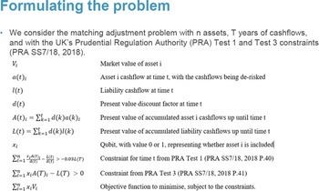
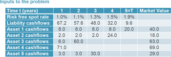
To formulate the problem, we consider the PRA Test 1 and Test 3, using n assets and t years of cash flows. Figure 2 defines tests, variables and parameters we will walk through. Start with the market value of an asset being V
i, the de-risked cash flows of asset i at time t being a(t)i, and l(t) being the liability cash flow at time t. There is a discount factor d(t) and A(t) is the present value of accumulated asset i cash flows up until time t. Similarly, L(t) is the present value of accumulated liability cash flows up until time t. We have a qubit assigned to each asset x
i here. Eventually it will take a value of zero or one, representing whether the asset is included or not. Next, we bring in the two constraints from the PRA. The PRA Test 1 states that the shortfall in asset cash flows cannot be more than 3% of the present value of liabilities at any time. This actually represents many constraints as it is a constraint for each time t. The PRA Test 3 is more straightforward, where you need sufficient assets by the end of the policy duration/project period. We now start introducing the objective function ∑x
i
V
i, which is what we want to minimise. The ∑x
i
V
i will be the combined market value of the chosen asset portfolio. The challenge is how to bring those constraints into the objective function.
Figure 2. The mathematical formulation for the PRA Test 1 and Test 3 and the variable and parameter definitions used in the example.
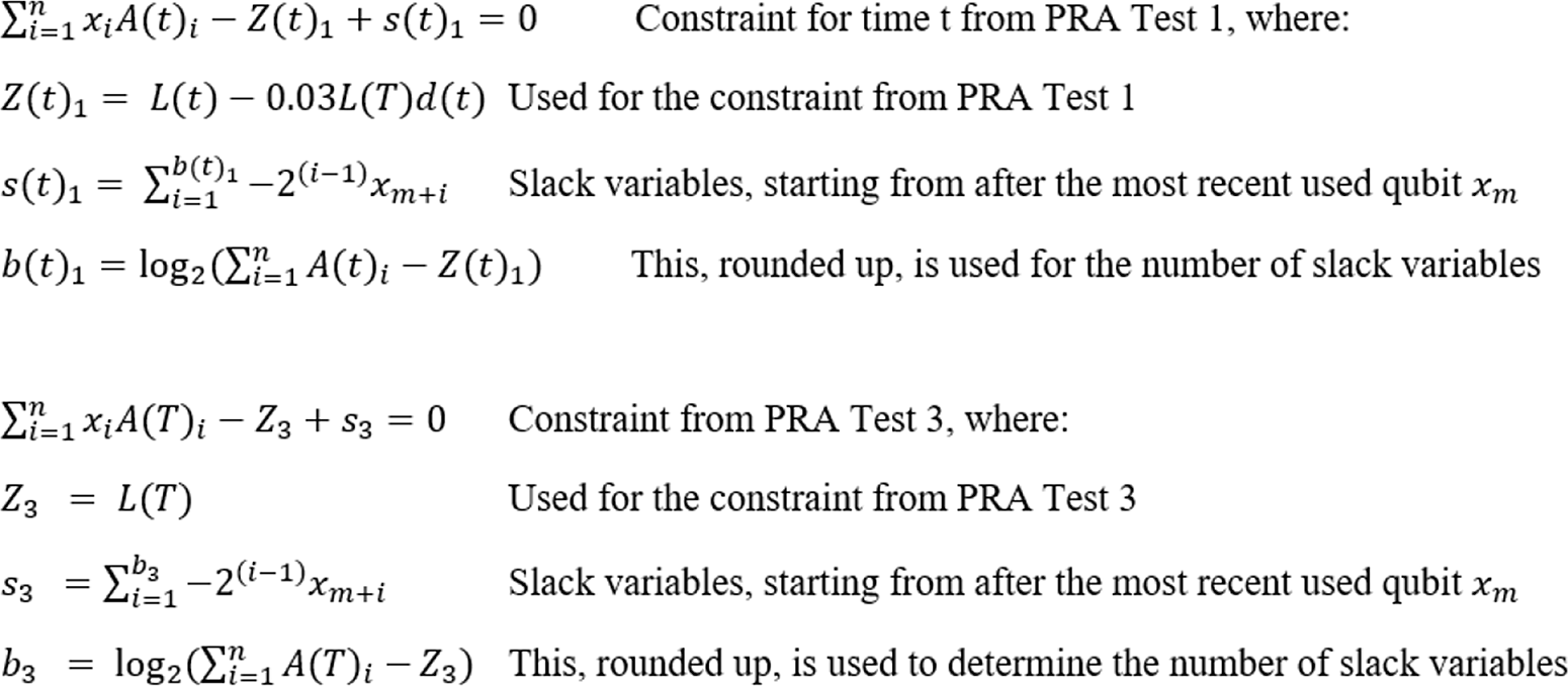
The way we do this is to first move all the terms to one side to create a quantity that is greater than zero and then introduce a number so that it becomes an equality equal to zero. This is when you introduce slack variables. In the case of the PRA Test 1, for a particular time t we move everything off to the left-hand side and re-express the formula (see Figure 3). We first create a function, Z(t), that generalises the problem based on the constraint in question and then we add s(t), which is the slack variable. The number of slack variables would represent a number that we know has an upper and lower bound: a lower bound of zero and an upper bound of some other number. This number can be written as the sum of various values of “two to the power of.” For example, eleven can be written as two to the power of zero plus two to the power of one plus two to the power of three. To each of those figures we can attribute a new slack power, a new qubit, so that an optimal solution would choose the right qubit combination of zeros and ones to get the right number so the constraint is met.
Figure 3. The re-expression of PRA Test 1 and Test 3.
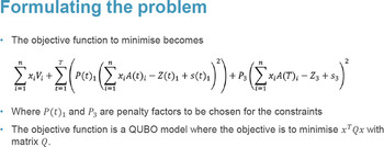
It is a similar process for PRA Test 3 where the formula can be expressed in much the same way (see Figures 2 and 3). The re-expressed constraints can then be collated together into a full objective function (see the formulae in Figure 4), which is the function we are trying to minimise. In the first term of the objective function you have the market value of the chosen assets. In the third term of the objective function you have P3 times a series squared. This term is a constraint and we are trying to minimise this. If you square this third term, the square is only minimised when it is zero. That is why we square that constraint, so that the constraint is met when this is minimised. If the constraint is not met, there will be a positive number and we want to penalise this. Because we are trying to minimise something, we therefore want to increase the number if the constraints are not met. That is why we have the P3 penalty factors in this case, and this parameter needs to be set large enough so it adequately penalises constraints that are not met. This must be the right amount, so that if it is almost fully met you will still find the correct minimum. So, setting the penalty parameter appropriately requires skill and judgement. An approach to setting this parameter might be to start with something, see what the results look like and adjust according using alternative penalty factors. The objective function is a QUBO model and it can also be written in matrix form. If you were to expand out the QUBO function there would be various combinations of x
i times x
j times the coefficients.
Figure 4. The objective function.
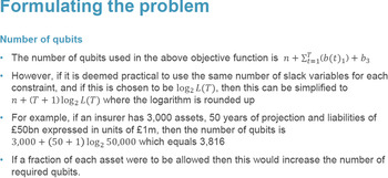
Before we move on and consider a worked example, just a comment on the number of qubits. The number of qubits used is given by the formula shown in Figure 5. In practice, it may be more practical to use the same number of slack variables for each constraint, as it is likely the number of slack variables will be similar for each constraint given that you are adding two to the power of some number each time.
Figure 5. The formula for the number of qubits used in the objective function.
As an example, if an insurer had 3,000 assets with 50 years of projections and liabilities of 50 billion expressed in units of 1 million, then the number of qubits would be around 3,800. That is below the number of qubits available in a quantum annealing computer. In practice, it is more complicated because the quantum annealing computer qubits are not all connected to one another, so the complexity of the problem may require more qubits. This is only looking at whether each asset is included fully or not at all. If we want to include a fraction of each asset, this is then a different challenge and would require an increase in the number of qubits.
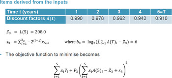
We will now finish on a worked example where we have five assets with five years of cash flows and only the PRA Test 3 constraint applying (see Figures 6 and 7 for the inputs, parameters and interim calculations of the example). We provide it the liability and asset cash flows, the market value of assets and assume the penalty factor to be 10. We incorporate the discount factors and calculate the Z function and number of slack variables (6). The objective function is shown in the formula in Figure 7. In order to solve for the optimal option, we need to convert the problem into a Quadratic Unconstrainted Binary Optimization (QUBO) matrix with various coefficients in front of x
i times x
j, as shown in Figure 8.
Figure 6. Inputs, parameters and values used in the worked example.
Figure 7. The interim calculations and objective function (reflecting PRA Test 3 constraints) used in the worked example.
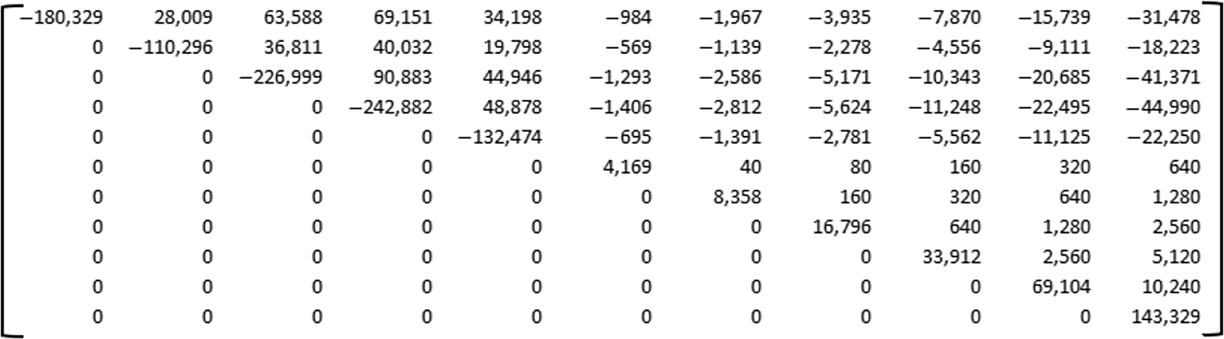
Figure 8. Worked example represented in QUBO form to try to minimise XTQx with the entries in row i and column j of the matrix being the coefficient of x
i
x
j of the objective function.
Row i and column j in this matrix gives the coefficient of x
i
x
j and then XTQX results in the formula from Figure 7. The leading diagonal is just the coefficients of x
i because x
i squared is equal to x
i, as x
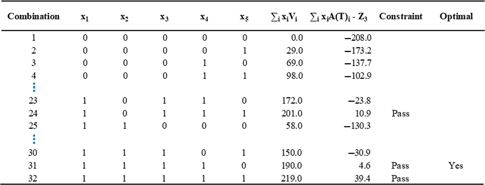
i is either a zero or one in the example. This formulation is now ready to go into a quantum annealing computer. As this is a relatively small problem, we can analyse it classically first to determine what we expect the outcome to be. For this purpose, we consider all possible combinations of the five assets, which will be two to the power of five (or 32) combinations. If you include all assets (32 combinations) then you are likely to have sufficient asset cash flows, but it is unlikely to be the optimum solution. When you start taking assets away, you get closer to the top of the table in Figure 9, where there is a low aggregate market value, but with insufficient assets for cash flows to meet the liability cash obligations. In this example, there are only three combinations that have sufficient asset cash flows for liabilities. The optimal combination is the one that passes the constraint and has the lowest market value of assets.
Figure 9. Expected results using “classical” analysis considering all combinations of assets and its results.
We now can see what the expected results are from a quantum annealing computer. In this case, there are eleven qubits: five assets and six slack variables, so 211 (2048) combinations. We can work out what the objective functional results would be just using Microsoft Excel.
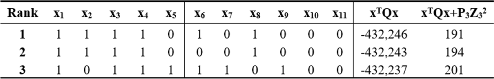
Using a quantum computer, the results show the most optimal combination being the one using the first four assets and not the fifth asset (see Figure 10). That is the same as the classical test earlier, so it gives us confidence that the objective function is correct. The next six qubits can be discarded because they are just slack variables. Once you have your solution, they are not needed anymore. As the quantum annealing results are the same as the classical analysis, the choice of a penalty factor often seems to be reasonable.
Figure 10. The results using a quantum annealing computer.
In conclusion, we feel that quantum computers have at least the potential to be useful for asset liability management. It is likely that the concepts can be more widely used for actuaries in general. It should be noted that finding a mathematical optimum is not the only thing to consider when choosing an optimal portfolio, but it is useful to know when making a decision. Finally, if we are able to determine new ways of finding optimal matching adjustments (perhaps considering a much wider set of assets), then this may lead to better retirement outcomes for people. That concludes the presentation. I will pass back to Andrew (Sharpe) to lead us into the Q&A session.
The Moderator: Thank you very much James (Sharpe) and Tim (Berry). We have got a few questions coming in. I am going to start off with a question from Jon Spain in London. “How near are quantum computers to practical use?” So maybe one of you could say a little bit about the hardware on which you ran the calculations you showed us.
Mr Berry: Quantum annealing computer is now being used in practice. The quantum computer we used has about 200 to 300 applications mentioned. Universal quantum computers will perhaps be useful at a later date. There are hopes for what that might do, like improving chemistry, which might help with analysing larger molecules that could lead to new ways of doing carbon capture and making transportation of electricity more efficient. This seems to be a bit further away, and universal quantum computing would seem a harder thing to build. With quantum annealing, there are approximately 5,000 qubits. They are not all connected, so if the problem you have is larger, then there is a potential to use a hybrid solution where one picks off parts of the problems that could be dealt with locally/via a classical computer, and parts in a quantum way. It is being used, but this is still new. It seems to have become available in the last few years.
The Moderator: Just to be clear, Tim (Berry), you did use a real quantum computer to do the calculation in your example?
Mr Berry: Yes.
Mr Sharpe: As Tim (Berry) said, they are usable now and people are using them for QUBO problems. If you can get a problem into the QUBO form, then you can apply that to the quantum annealing computer and solve it in a much quicker time.
The Moderator: We have a question from Malachy McGuinness: “In your example, you could validate the answer by classical methods and see the right answer. That enables you to conclude on the appropriateness of your penalty factor. If you suppose the problem was too hard to compute under a classical method, how would you know that you have chosen the right penalty factor?”
Mr Berry: That is a great question. I think that is a challenge of quantum computers. There was a story, a few years ago, on whether universal quantum computers had claimed to have solved something better than any supercomputer, but it was debatable because it was hard to verify. There are errors with quantum computing. You may not necessarily get the perfect results every time, and if you run the same problems/scenarios, you may not get the same results. There are physical hardware constraints where the processors need to be kept at temperatures of almost absolute zero. There are many more errors than you would get with a classical computer and that remains a challenge. In the case of matching adjustments, some of the methods that James (Sharpe) mentioned earlier on operations research, you potentially could verify the problem given sufficient time.
The Moderator: A question in from Martin White about Periodic Payment Orders (PPO). You might be familiar with those. They are awarded to victims in various sorts of accidents, and very often they have cash flows for life, linked to some inflation index (e.g. maybe an index of wages for care providers). There are some questions about what a suitable set of assets might be, either for an insurer who has the liability, or the victim who may invest their respective lump sum. It is not really a quantitative computing question. It is more an ALM question but we would be interested to hear your thoughts on this.
Mr Sharpe: Yes, ideally you will have assets linked to indices like the Annual Survey of Hours and Earnings (ASHE), but I do not believe there are any. The problem is how to minimise the capital requirement based on that basis risk between the actual index and RPI or CPI assets you might be matching it with. I do not think there is a solution at the moment, where you match liability based on an index that you do not have any assets based on. You will encounter a basis risk problem if you use RPI to try to match the liabilities that are growing at a different inflation rate. Something that could be done, as an example, is that you could hold more assets than liabilities, which is in principle what you probably have to do with any capital events. It might be possible to invest in assets tracking the ASHE index. I am surprised that no company has done that to date. You could also merge the PPO liabilities with other liabilities, so that it reduces the size of the basis risk when you look at the full portfolio of liabilities. If you have some measure of how much basis risk you can allow for, and combine your PPOs with another block of non-inflation linked liabilities, then as a proportion of the full block, it hopefully would be a smaller amount. It is a difficult problem though without assets backing ASHE.
Mr Berry: One thing I like about the question is that it considers areas that are less familiar. Of course, we have picked an example that we are fairly familiar with, but potentially actuaries could consider things like liabilities associated with nuclear power station decommissioning, which are large liabilities in the distant future, and what assets might be needed. When enough qubits become available, quantum computing might also be able to consider the entire universe of investible assets.
The Moderator: We have had a few more questions coming in about other applications. Somebody is suggesting dynamic portfolio optimisation. I think there have been papers presented previously on high frequency trading applications. I am interested in any comments you have about this.
Mr Berry: One thought occurs to me. We have been in contact with the quantum computing company, and there seemed to be very few finance-related applications. In fact, this was the first insurance-related one they knew of. If someone comes up with some new ideas to solve a problem with quantum computers, they probably will be the first to do it. It is an interesting area for those who might be interested in those ideas.
Mr Sharpe: In terms of other applications, if you can get that problem into the QUBO form, then that quantum annealing computer can solve it, but the general-purpose quantum computers can do different algorithms as well.
The Moderator: We have a question about other applications for economic scenario generators, forecasting interest rate curves and SOP rates. Do either of you have anything to say about that?
Mr Berry: It is less clear to me at this stage whether it can perform, and substitute for, Monte Carlo simulations. The types of problems it is well-suited to solving have discrete values. The QUBO is binary, but one of the problems it is particularly good at is the “travelling salesperson” problem, where you have to pick the quickest route and these have discrete solutions. This is the kinds of things that can be done in seconds with quantum computing, where classical computers might take minutes. If Monte Carlo simulation could be put into a QUBO form, then this could be theoretically done using a quantum computer.
The Moderator: Another question from the audience. In your optimisation example, this is over discrete variables that could be zero or one. James (Sharpe) mentioned the potential of using continuous variables where you hold a proportion of your portfolio in an asset and that proportion can be between zero and one, or any real value in between. I wondered if you could comment on the discrete continuous contrast.
Mr Sharpe: Yes, it can be done, this just entails plugging in a whole asset or not. A simple solution would just be to add more qubits for each decimal place, so you would have fractions of each asset. That would give the same answer to the number of decimal places you want for fractions of assets.
Mr Berry: A discrete option has become available, so rather than just zero and one, you could give it maybe 50 different possible outcomes. It will of course use up more qubits. As far as we are aware, we don’t know a way of getting a solution equivalent to a continuous outcome. That could be a new problem that could be solved. Potentially you could have 99% of the asset allocated to one qubit, and 1% to another qubit, and could there be any iterative way of homing in on the right continuous solution using potentially a combination of classical and quantum computing? I think this is an open question.
The Moderator: We have got a few questions about the practicalities of quantum computing and what quantum computers you used. Did you have to call in a few favours with somebody at a university? Can you just go online and find one that charges by the second? How does it work in practice? Is there a URL you can share?
Mr Berry: Yes, they are now available. There are several well-known companies who are building this capacity. You can search online and find them. We probably won’t mention the individual ones, and keep it general, but they are available to find on the internet. The one we used could be accessed through the internet. You have to write some python code and provide it with the QUBO structure. It allows a certain amount of free usage.
The Moderator: We have got a question here from Gerard Kennedy who is commenting on cryptography and encryption, and security for financial trades. They are asking for your comments on whether this is going to lead to an arms race, where access to quantum computers makes it easy for bad actors to crack codes, and therefore the good guys must keep strengthening their codes. Any thoughts on that?
Mr Sharpe: This is what I thought of when I looked at this. If you can solve that QUBO problem, a discrete problem that is hard for classical computers, then you can basically solve it instantly, and a lot of those cryptography problems can be solved straight away. The hardware for some of the bigger problems isn’t there, and the number of firms having sufficient hardware for a QUBO problem is small. If somebody was doing this at the moment, it would probably be easy to find them. I suspect that it is going to be something that happens in the next few years.
Mr Berry: People are saying that the security of the internet could be at risk unless tools are developed. One area I think is interesting about cryptography is that with the quantum mechanics properties, you can tell if your encrypted message has been intercepted using quantum methods, which I find fascinating.
The Moderator: I am going to breach protocol and answer a question myself on whether quantum mechanics is being taught in universities given I happen to be a university teacher. I believe the answer is “no,” but we certainly teach a lot more coding in R, Python and other tools now compared with five or ten years ago. I am not, and I would not be able to, teach quantum computing, but that is a good suggestion. A lot of these changes start from educating actuaries and then waiting 30 years.
The Moderator: Another question here. The banking sector seems to be investing more in quantum computing than insurers are. Apart from the obvious fact that the banking sector is bigger than the insurance sector, have you got any comments on whether you think there might be more applications in banking than insurance?
Mr Sharpe: On the ALM matching problem, a lot of insurers are using methods developed in 1938 rather than the ones developed in the 1980s or in 2011. Maybe some of that is because papers on operations research were not very widely read by actuaries. It is not on the actuarial syllabus, so it has been a bit ignored. When you talk to people at the big banks, they are using these methods. They are spending a lot of time and effort on these kinds of approaches. Some of it is down to actuarial mentality where they like to have something that is prudent, but not necessarily quantified. This is something people are uncomfortable with – quantifying the level of prudence. In this presentation, we have said that if you are able to optimise and know where the limit is, this is useful information, even if you don’t use it. Banks have been using it for this purpose, but this has probably been an area where actuaries have ignored developments a bit and banks have been more focused on those same developments. If it is the same phenomenon with quantum, that would not be surprising, but it probably is something that we should try to reverse. I think insurance companies should be looking at this as well.
The Moderator: Thank you. We have got a question from a member here about the rate of increase in technology. Is there a Moor’s law type of relationship where every eighteen months, the number of qubits is doubling?
Mr Berry: That is a great question. Computer scientists do have a great track record in this respect. It appears that universal quantum computing is a very difficult thing to achieve, but who knows? You do not necessarily need millions of qubits. Once you get to a certain number, you can do some amazing things. I may have mentioned earlier, I think tasks related to chemistry might be one of the most amazing things it has potential for. Timescale wise, I don’t know. In quantum annealing, I mentioned there was the hybrid solution that can take very large problems, so that is an area of interest too.
Mr Sharpe: I saw some discussions a few year ago from a well-known physicist who said, around 2019, that this is just not going to happen and quantum computing would be a bit like nuclear fusion, where it was theoretically possible but never happened. Then the same person two years later gave a presentation where they said “Look, hold on. This has already happened now.” It was something they thought two years prior would not happen, but they are now saying that actually there are quantum annealing computers with 5,000 qubits. It is very difficult to know whether we are either absolutely on the cusp of something enormous or more like the nuclear fusion situation that never took off. It does feels like a small probability now that it proceeds like nuclear fusion.
The Moderator: Another question from Bea Shannon about Solvency II reform, in connection to the UK and the recent consultation from Her Majesty’s Treasury. Do you think there is going to be any impact of quantum computing and ALM that we can do, now that we do not have to follow the previous European regulations in this area?
Mr Sharpe: It obviously depends on what the new problem is and whether it has changed. In an extreme scenario where there is no requirement whatsoever, then you still want to have the best way of managing the business. Tim (Berry)'s example on the quantum side is just showing how this could work, but if the constraints were not regulatory constraints, a pension fund or an insurance company would still want to be well matched. It still makes sense to manage the matching using constraints for things you are worried about.
The Moderator: Thank you for that. We have got a comment here you might want to reflect on, which is that Redington immunisation limits profits as well as losses. In your objective function, does that eliminate upside as well as downside?
Mr Sharpe: You are maximising the yield on the assets, but you can introduce a constraint. For example, you could have one of your constraints set such that you would never lose more than a certain amount in a yield curve stress.
The Moderator: We have a question from Tahira Hussain about whether the IFoA needs to be doing something on quantum computing. Now of course, we have already done something because we have got this paper out. What do you think the next steps should be? Do we need a panel to keep looking at it, something like the CMI? How will we encourage actuaries to use it more widely?
Mr Berry: I feel having knowledge of the QUBO model feels like something suitable for actuaries. It is mathematical, and perhaps less computer science. Universal computing is a very unusual way of programming, and maybe that is venturing more away from the actuarial discipline and more into computer science. It is certainly a new area and it would be great if the IFoA were to create interest through training and working parties.
The Moderator: I am going to tie in a question of my own about classical ways of solving the same problem. The problem that you stated in your original problem with continuous variables is a quadratic programming problem. Those familiar with these types of problems would know that an established way of solving it would involve writing down conditions and then solving it using a simplex algorithm, but there is a bit of clever mathematics as a prelude to doing the computing. If you just throw a computer at it, you might not get very far. It seems that with quantum computing you need to do less homework. You have brute force and out comes an answer. Do you think that is going to save us thinking time? Is that a good thing or a bad thing and would you like to compare and contrast those different approaches?
Mr Berry: It does seem that way. In the case of quantum annealing, the skill is formulating the problem in QUBO form, which is mathematical, and perhaps an actuarial-type skill. Once you have it, you can then run it. There are certain parameters associated with running it like how many times it is run and other details, but it is not fully just about computing. Formulating a problem is part of the challenge I see.
Mr Sharpe: In the classical problem there the two steps. First is defining the problem and second is finding the algorithm to work its way through to find the optimum. The challenge here is to get the problem into QUBO form, after which the quantum computer finds all the answers straight away and effectively takes out one of the steps. One challenge is also to keep the number of qubits to a minimum, because these are limited at the moment. Tim (Berry) mentioned 5,000 for quantum annealing computers earlier. When that goes up to 100,000 it won’t be a problem, but currently, if you can find ways to express the problem with as few qubits as possible it is beneficial, because that is a challenge at the moment.
The Moderator: Related to that, we have got a question from Rahul Khandelwal about selecting the numbers of qubits and selecting penalty factors. That is a human input. Is there a risk of biasing the results due to subjective inputs?
Mr Berry: Yes, you can argue that good judgement is required. It is expected that you would run that many times to check and get a feel for the results. Then, there is the challenge when the problem becomes too hard to check classically in any way and how you know it is a suitable answer. It would seem to be a skilled task which, I would say, does relate to the actuarial skill set.
The Moderator: We have a question about how practical it is to keep updating this on a daily basis. When you have done it once, how much could then be automated?
Mr Sharpe: I thought it could be automated relatively easily. It is like the classical form. Some firms running it have some challenge to get it into the right format, but it is the same thing for the quantum form: if you set it all up properly you can automate it at a press of a button similar to the classical method.
The Moderator: Some of you on the call may have heard of simulated annealing as being an optimisation tool, which is used for particularly difficult optimisation questions. I would come across it in calibrating economic scenario generators for complicated implied volatility surfaces. Apart from just the common use of the word annealing, has simulated annealing anything to do with quantum annealing? Annealing is what we do to metal, isn’t it, when you are cooling iron and you give it a bash so that it settles in a crystalline form that is suitable for application. What are all these different annealing algorithms about and how do they link up?
Mr Berry: That is a great question. Simulated annealing can be done classically on a classical computer. Essentially the way it works is you might be trying to find the lowest points in a valley, and you randomly choose a direction to move in. If it is a lower point, then you move to that point. If it is a worse move, then you may still move there but the probability reduces with the so-called “badness” of the move. Quantum annealing can be compared to that. You might start at the top and try to seek the lowest point in the valley, but it has some advantages. Because of superposition, you can start in many coordinates. When you get into some local minimum, then that is where things like quantum tunnelling mean you can go straight through the hill rather than having to require the energy or the probability to climb over the hill. That is why it is seen as a better way of simulating.
The Moderator: We have a question here about parallel computing compared to quantum computing. Is there an analogy between quantum computing, where all the states are there at once until you resolve the wave function, compared with parallel computing where a large number of chips are processing in parallel? Is there an analogy/comparison there?
Mr Berry: I suppose they can be compared, but I think the hope is that quantum computing will be better than super computers in future. It has substantial potential given the number of states that could simultaneously exist. Even the best supercomputers will never reach that point. I do see the point about parallel computing, which we use a lot in valuation when we are trying to value many policies. We just often have a computer that sets off many computers to do the evaluation at once.
The Moderator: It seems that we have answered all the questions that people had. Tim (Berry) and James (Sharpe), were there any closing remarks that you would like to make to inspire or encourage us before we wind up the session?
Mr Sharpe: I had one comment and that was to encourage people to start having a look at the topic in this paper. It is obviously a simple example. It has been tested on a quantum computer, but as Tim (Berry) was saying earlier, that QUBO model is one model. This is just starting, so there will be other algorithms used that apply to other uses. It is worth reading up on for your applications that you are looking at. It is a new tool that actuaries should be starting to look at.
The Moderator (closing the discussion): In that case, I am going to thank Tim (Berry) and James (Sharpe) for a fascinating and wide-ranging presentation here. You have really helped us think through some quite broad issues that are outside the main areas of expertise for many of us, so we are very grateful for the research you have done, the effort that you have put in to writing this paper and the trouble you have taken to present it to us today. Thank you also to those of you who dialled in from around the world.


 This is an Open Access article, distributed under the terms of the Creative Commons Attribution licence (http://creativecommons.org/licenses/by/4.0/), which permits unrestricted re-use, distribution, and reproduction in any medium, provided the original work is properly cited.
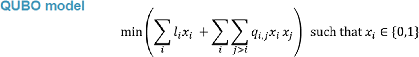
 You have
Access
You have
Access
 Open access
This sessional meeting discussion relates to the paper presented by Tim Berry and James Sharpe at the IFoA sessional webinar held on 5 July 2021. The Moderator (Mr A. D. Smith, Hon F.I.A): Good afternoon, everybody, and welcome to this sessional meeting on “Asset Liability Modelling in the Quantum Era.” My name is Andrew Smith and I teach Actuarial Science at the University College Dublin. Welcome especially to those of you who are dialling in from overseas.
We have two speakers today: Tim Berry and James Sharpe. Tim is a consulting actuary. He specialises in valuation and pricing models in life insurance, primarily in reinsurance. Tim’s real strength is in creating insightful, user-friendly and efficient models. He has worked in Hong Kong and Tokyo for many years. He is now back in the UK, but still has a good portfolio of international clients. He regularly chairs actuarial learning events and has an amateur interest in physics and hiking in warm places, which today probably includes London.
James Sharpe is also a consulting actuary. He has more than twenty years of actuarial experience, and recently he has done a lot of work on calibrating internal models on matching adjustment portfolios and asset liability matching. He chairs the IFoA’s Extreme Events Working Party, of which I also happen to be a member.
So without further ado, I am going to hand over to Tim (Berry) and James (Sharpe) to present to us on the topic of “Asset Liability Modelling in the Quantum Era.”
Mr J. A. Sharpe, F.I.A. (introducing the paper): There are six items on the agenda. For the first item, “Introduction – What is Asset Liability Modelling (ALM)?”, we talk through what this means and the general principles used under ALM. The second section is on “Specification of the ALM Problem” and specifying what we are trying to do in ALM. In section three, we look at “Early Attempts to Solve the ALM Problem,” examining how actuaries have been looking at this problem for the last 300 to 400 years and how the approach has evolved over the years into what people do today. The fourth section on “Current Solutions to the ALM Problem” covers the solutions we see in insurance companies operating in the UK, Europe and the US today. Section five, which forms the majority of this presentation, is on “Quantum Computing” and how this can be used to solve the ALM problem. Section six contains our conclusions.
So, what is ALM? To address this, we took a set of points first described by Arthur Bailey in his paper from 1862. We liked these points because they were relevant at the time, but remain relevant today, 160 years later. Arthur Bailey’s paper was the first articulation of efforts to deal with the ALM problem. The first point that Mr Bailey came up with is the consideration of default risk. A primary consideration is to minimise default risk for assets that we are considering for backing our liabilities.
The second point Mr Bailey came up with is that we would prefer a higher yield to a lower yield. So, provided we have controlled our default risk and have a good understanding of this, a higher-yielding asset is preferred to a lower-yielding asset, for the same security of capital.
The third point Mr Bailey came up with was that some of the assets should be readily convertible or liquid. If we only have illiquid assets, then this can create problems due to changes in liabilities or short-term claims/outgoings.
The fourth point raised was the concept of a liquidity premium, which is still very much around today, where illiquid assets typically would have higher-yielding returns than assets that are more liquid but of the same security/default risk. Even in 1862 people were looking for the same type of liquidity premium that continues to be sought out today, to back the long-term liabilities. Finally, the fifth point, which perhaps is not so common today, is that capital should be employed to aid the life assurance business itself.
The above principles were a clear articulation of the key underpinnings of ALM and what an insurer might try to do when selecting assets to back long-term liabilities.
We now proceed to the section dealing with the specification of the ALM problem. We try to minimise the value of the assets to back our liabilities, subject to several constraints. Minimising the market value of the assets is the same as maximising the yield on those assets. The constraints we have noted are typically what you would expect under regulatory requirements or similar to those that the management of an insurance company might be focused on. These would be items like minimum security requirements. For example, with a matching adjustment portfolio, there is a limit on BBB rated assets where you can have a “matching adjustment” (MA) higher than a BBB asset.
Insurance companies themselves might also have specific limitations on assets of a particular credit rating. For example, not all investments need to be allocated in BBB or above assets. It may be possible to invest in assets with other ratings as well. There could also be a maximum exposure to interest rate risk to limit the impact of interest rate movements, and similarly for inflation or currency risks. There could also be a requirement to maintain a minimum level of liquid assets, such as gilts or cash, so that you can meet your liquidity requirements. The minimum present value of asset cash flows compared to liability cash flows is also a requirement on the MA portfolio, as well as other requirements. These include a minimum cash flow mismatch in any given year, so that over any year during the term of the liabilities there is not a large deficit which might need to be subsidised by a large surplus in another year. Lastly, there may also be some constraints to minimise capital requirements, for example regulatory or risk capital requirements.
The next section outlines a brief history of ALM that prepares us for the discussion about quantum computing. There is a quote from Charles Coutts in 1933 where Mr Coutts, who was the President of the Institute of Actuaries, said “An attempt should be made to ‘marry’ the liabilities and the assets as far as possible.” This was picked up in a book by Craig Turnbull entitled “A History of British Actuarial Thought,” pointing out that no quantitative method had been introduced in ALM until 1933. For over 70 years it had still been looking at qualitative points and principles rather than mathematical calculations. But the move to quantitative methods happened in 1938 with the Macaulay Duration. In principle, if the asset time-weighted average of cash flows was matched with that of the liability time-weighted average of cash flows you could argue that the asset and liability positions were matched. Items like changes in interest rates could be minimised by having a closely matched time weighted average of your cash flow, that is by matching the duration. It was not until the 1950s that this matching of durations was formalised, and that was done so by Frank Redington in his immunisation formula. It is a very well-known formula used by many actuaries to this day.
Looking at Redington’s immunisation formula, the value of liabilities is set equal to the value of assets. Any asset amounts above this are not subject to this method and are considered outside this framework. Then, looking at the present value of the asset and liability proceeds, the portfolio is de-sensitised to small changes in interest rates. This means that if interest rates move, we want to ensure the surplus (amount of assets over liabilities) is not negatively reduced. The way Mr Redington did this was to use Taylor’s approximation for a small change in interest rates. A change in the value of assets with respect to interest rates, minus the change of value of liabilities with respect to interest rates, can be approximated to by Taylor’s theory. Redington concludes that if you set the first derivatives (in the Taylor series) to zero and the second derivative to greater than zero, then in cases of a small interest rate change, you would make a small profit/observe a small increase in your surplus subject to small changes in interest rates such that none of the higher order terms impacts (in the Taylor series expansion) surpasses the impacts of the first two derivatives. This is quite a simple method, but also very effective.
In Redington’s paper, he talks about immunisation with respect to interest rates, but it could also be applied to other risks such as inflation or currency risk. Redington notes that there are infinitely many solutions to his immunised equation, but he does not comment as to which solutions might be preferable, such as maximising yield whilst minimising credit risk. You are still left with this combination of quantitative methods in unison with Bailey’s qualitative descriptions from 1862. Furthermore, if we are choosing solutions based on single present values, it is possible to have cash flow mismatches in particular years that could cause liquidity issues. Those problems are there because people did not have the computing power they now have. Following a 20-year period after the World War II, we did see huge progress in computing power, which led to new solutions and the first introduction to operations research methods. There was a huge level of research during the World War II on operations research methods, where computers were used in places like Bletchley Park. At the end of the war, the people who worked in the field produced a lot of papers that went out into industry, including insurance companies. In principle, operations research is all about maximising or minimising certain parameters subject to a number of constraints. This is an ideal set of tools for the ALM problem we have talked about where we are minimising the market value of the assets subject to a list of constraints. The simplest algorithm you might use is to consider all possible combinations of assets and see which gives you the best value(s). If you use a non-quantum computer to do this, it might take a significant amount of time. For example, if you have 100 assets, you get 2100 possible combinations of those assets and that is only if you consider the possibility of investing 100% in each asset, and not considering partial holdings, for example, 50% of one asset and 50% of another, which would mean many more combinations. 2100 is approximately equivalent to 1030 possible combinations.
Whilst that is an algorithm that could be written, it cannot be solved within a tangible timeframe. These operations research techniques are all about identifying algorithms that can reduce that timeframe by narrowing down the number of scenarios you look at. This is done by dismissing a large number of scenarios from the outset. Using these methods, large pensions or insurance company portfolios might only take a few minutes to run.
There are two key parts of an operations research type problem you need in order to find a solution to the ALM problem is. The first is to identify and define the problem in mathematical terms, and that can often be visualised in n-dimensional spaces. In our example we use two assets and try to look at the optimism proportion of these two assets, which would maximise a return subject to a number of constraints. If you had 500 assets, it would be a 500-dimensional shape. There is a whole host of possible algorithms you could use depending on whether the problem is linear or non-linear. Once you define the shape and specify the problem, then you would apply this algorithm and it would find what you hope is the maximum. It either is the maximum or, if it is a non-linear problem, it might be only close to the maximum.
This is a description of the current ALM practices that insurance companies are using. As mentioned previously, such an algorithm might take several minutes to run and you can effectively solve this problem. It just narrows down the number of possible solutions it looks at and that means it goes from taking an impractical amount of time, by considering all possible combinations, to taking five or ten minutes. It is quite an efficient process, but if you are a large insurance company, you might want to run 500,000 scenarios on your portfolio. If you wanted to optimise in every one of those scenarios, taking 10 minutes to do each of these optimisations would still be an unworkable amount of time. In order to resolve this problem, we need to look at alternative approaches. The next step that is being considered is quantum computing, where timeframes are vastly smaller for these kinds of problems. So, to talk us through that next stage, I will hand over to Tim (Berry).
Mr Tim Y. Berry, F.I.A.: Before we consider how a quantum computer can solve the ALM problem, we will first consider some of the properties of quantum mechanics that are relevant to quantum computers.
The Copenhagen interpretation of quantum mechanics was devised in the 1920s by Bohr and Heisenberg. In this research, microscopic quantum objects were deemed to not have definite properties prior to being measured. The wave function is a mathematical representation of the system, and from this you can define probabilities of the measurement results. When you measure the objects, the wave function collapses and becomes certain in properties. In our illustration, we show a photon on a plane, and the vertical axis is the probability of where it might be. When you look at it, it collapses into a particular place, but before you looked at it, it had a range of probabilities.
The two key features of quantum mechanics are “superposition” and “entanglement.” To get an idea about superposition, we show an experiment in our diagrams where you create a photon at the source and send it towards a partially reflective mirror where there is a 50% chance it could go into box A or a 50% chance it could go into box B. Each of the boxes has a slit, which are opened simultaneously, through which the photon then leaves the box and heads towards a screen where it is measured as a dot. If the experiment is repeated many times, one photon at a time, then an interference pattern appears on the screen. The results of the pattern shown indicate that each photon was originally in both boxes at the same time. This principle of the photon being in two positions at the same time is an example of superposition.
The other key property of quantum mechanics is “entanglement.” Imagine if you create two electrons in such a way that they have opposite spin properties, so if the first electron is an “up” electron, then the other electron is a “down” electron. Imagine that you create two electrons (one with an “up” spin and another with a “down” spin) and put them in separate boxes, and then keep one box and send the other box to the other side of our galaxy. If we open the box in front of you and you discover it is an “up” electron, then you know that the other electron must be a “down” electron. What is surprising about this is that before you looked at that electron, it was in its superposition state of being “up” and “down.” By looking at it, it became an “up” electron which means you have made something else at the other side of the galaxy change into a “down” electron. This was obviously unexpected and led to the EPR (Einstein-Podolsky-Rosen) paradox in the 1930s, which described this as “spooky action at a distance” and suggested that the wave function is not how reality is. In the 1960s, John Bell formulated the “Bell theorem,” which was later tested and validated in the 1970s. Although this experiment has been tested to a very high degree of accuracy, what is still not fully understood is what is occurring at the collapse of the wave function. Whilst the Copenhagen interpretation is the most widely accepted interpretation, there are others too, most noticeably the many-worlds theory, where instead of the wave function collapsing, a parallel universe might emerge at that time.
Next, we move onto some ideas behind quantum computing. Quantum computers have quantum bits or qubits, and these can be compared to classical bits. A classical bit, in a classical computer, can take a value of zero or one, whereas the quantum bit can be in a superposition state of both. It is both zero and one, until it is measured, and its wave function collapses, and then it becomes either one or zero. Using entanglement, it is possible to create a set of connected qubits. If we consider three bits, then there are 23 possible combinations. A classical computer might perform a calculation on each combination sequentially, whereas quantum computers can use and calculate all the states at once. If this example was extended to 1,000 bits then a classical computer would not be able to manage this. In reality, quantum computing is more complicated and, for example, if you were to look at the qubits, you would imagine it would collapse into one of the many combinations that may be of no use. You have to control them in a certain way, and it is therefore a new type of programming. This works in a very different way to the current classical computers.
There two main types of quantum computing. The first is quantum annealing, which is used for optimisation problems and works by putting a system in a high-energy state. The energy is then lowered with the aim of seeking a global minimum. Quantum properties such as quantum tunnelling and superposition help the system escape a local minimum. At the current time, the number of qubits for Quantum annealing computers is of the order of 5,000.
Universal quantum computers are the second type and are different from quantum annealing. They have a wider scope of applications and involve controlling individual key bits using quantum circuit operations. At the current time, the number of qubits is of the order of 100. For ALM, we feel that quantum annealing is the area of interest.
We will now bring it back to the ALM problem that James (Sharpe) introduced earlier. We will try to solve the Solvency II MA problem. This is a problem of selecting the subset of assets so that their combined market value is minimised, subject to the constraints from the regulator: the asset de-risked cash flows must be adequately matched to the insurer’s liability cash flows. This can be formulated as a “Quadratic Unconstrained Binary Optimisation” (QUBO) problem, which can then be put through a quantum annealing computer. The QUBO model shown in Figure 1 outlines all possible ways of multiplying x i by x j, and coefficients in front of these define the problem. We are using a quantum computer to work out what the x i’s should be, and as they are either a value of one or zero, this also means that x i squared is x i, and that is why we have a linear term there. The model can then be expressed in matrix form, and this will be illustrated in an example later.
Figure 1. Mathematical formulation of the QUBO model.
To formulate the problem, we consider the PRA Test 1 and Test 3, using n assets and t years of cash flows. Figure 2 defines tests, variables and parameters we will walk through. Start with the market value of an asset being V i, the de-risked cash flows of asset i at time t being a(t)i, and l(t) being the liability cash flow at time t. There is a discount factor d(t) and A(t) is the present value of accumulated asset i cash flows up until time t. Similarly, L(t) is the present value of accumulated liability cash flows up until time t. We have a qubit assigned to each asset x i here. Eventually it will take a value of zero or one, representing whether the asset is included or not. Next, we bring in the two constraints from the PRA. The PRA Test 1 states that the shortfall in asset cash flows cannot be more than 3% of the present value of liabilities at any time. This actually represents many constraints as it is a constraint for each time t. The PRA Test 3 is more straightforward, where you need sufficient assets by the end of the policy duration/project period. We now start introducing the objective function ∑x i V i, which is what we want to minimise. The ∑x i V i will be the combined market value of the chosen asset portfolio. The challenge is how to bring those constraints into the objective function.
Figure 2. The mathematical formulation for the PRA Test 1 and Test 3 and the variable and parameter definitions used in the example.
The way we do this is to first move all the terms to one side to create a quantity that is greater than zero and then introduce a number so that it becomes an equality equal to zero. This is when you introduce slack variables. In the case of the PRA Test 1, for a particular time t we move everything off to the left-hand side and re-express the formula (see Figure 3). We first create a function, Z(t), that generalises the problem based on the constraint in question and then we add s(t), which is the slack variable. The number of slack variables would represent a number that we know has an upper and lower bound: a lower bound of zero and an upper bound of some other number. This number can be written as the sum of various values of “two to the power of.” For example, eleven can be written as two to the power of zero plus two to the power of one plus two to the power of three. To each of those figures we can attribute a new slack power, a new qubit, so that an optimal solution would choose the right qubit combination of zeros and ones to get the right number so the constraint is met.
Figure 3. The re-expression of PRA Test 1 and Test 3.
It is a similar process for PRA Test 3 where the formula can be expressed in much the same way (see Figures 2 and 3). The re-expressed constraints can then be collated together into a full objective function (see the formulae in Figure 4), which is the function we are trying to minimise. In the first term of the objective function you have the market value of the chosen assets. In the third term of the objective function you have P3 times a series squared. This term is a constraint and we are trying to minimise this. If you square this third term, the square is only minimised when it is zero. That is why we square that constraint, so that the constraint is met when this is minimised. If the constraint is not met, there will be a positive number and we want to penalise this. Because we are trying to minimise something, we therefore want to increase the number if the constraints are not met. That is why we have the P3 penalty factors in this case, and this parameter needs to be set large enough so it adequately penalises constraints that are not met. This must be the right amount, so that if it is almost fully met you will still find the correct minimum. So, setting the penalty parameter appropriately requires skill and judgement. An approach to setting this parameter might be to start with something, see what the results look like and adjust according using alternative penalty factors. The objective function is a QUBO model and it can also be written in matrix form. If you were to expand out the QUBO function there would be various combinations of x i times x j times the coefficients.
Figure 4. The objective function.
Before we move on and consider a worked example, just a comment on the number of qubits. The number of qubits used is given by the formula shown in Figure 5. In practice, it may be more practical to use the same number of slack variables for each constraint, as it is likely the number of slack variables will be similar for each constraint given that you are adding two to the power of some number each time.
Figure 5. The formula for the number of qubits used in the objective function.
As an example, if an insurer had 3,000 assets with 50 years of projections and liabilities of 50 billion expressed in units of 1 million, then the number of qubits would be around 3,800. That is below the number of qubits available in a quantum annealing computer. In practice, it is more complicated because the quantum annealing computer qubits are not all connected to one another, so the complexity of the problem may require more qubits. This is only looking at whether each asset is included fully or not at all. If we want to include a fraction of each asset, this is then a different challenge and would require an increase in the number of qubits.
We will now finish on a worked example where we have five assets with five years of cash flows and only the PRA Test 3 constraint applying (see Figures 6 and 7 for the inputs, parameters and interim calculations of the example). We provide it the liability and asset cash flows, the market value of assets and assume the penalty factor to be 10. We incorporate the discount factors and calculate the Z function and number of slack variables (6). The objective function is shown in the formula in Figure 7. In order to solve for the optimal option, we need to convert the problem into a Quadratic Unconstrainted Binary Optimization (QUBO) matrix with various coefficients in front of x i times x j, as shown in Figure 8.
Figure 6. Inputs, parameters and values used in the worked example.
Figure 7. The interim calculations and objective function (reflecting PRA Test 3 constraints) used in the worked example.
Figure 8. Worked example represented in QUBO form to try to minimise XTQx with the entries in row i and column j of the matrix being the coefficient of x i x j of the objective function.
Row i and column j in this matrix gives the coefficient of x i x j and then XTQX results in the formula from Figure 7. The leading diagonal is just the coefficients of x i because x i squared is equal to x i, as x i is either a zero or one in the example. This formulation is now ready to go into a quantum annealing computer. As this is a relatively small problem, we can analyse it classically first to determine what we expect the outcome to be. For this purpose, we consider all possible combinations of the five assets, which will be two to the power of five (or 32) combinations. If you include all assets (32 combinations) then you are likely to have sufficient asset cash flows, but it is unlikely to be the optimum solution. When you start taking assets away, you get closer to the top of the table in Figure 9, where there is a low aggregate market value, but with insufficient assets for cash flows to meet the liability cash obligations. In this example, there are only three combinations that have sufficient asset cash flows for liabilities. The optimal combination is the one that passes the constraint and has the lowest market value of assets.
Figure 9. Expected results using “classical” analysis considering all combinations of assets and its results.
We now can see what the expected results are from a quantum annealing computer. In this case, there are eleven qubits: five assets and six slack variables, so 211 (2048) combinations. We can work out what the objective functional results would be just using Microsoft Excel.
Using a quantum computer, the results show the most optimal combination being the one using the first four assets and not the fifth asset (see Figure 10). That is the same as the classical test earlier, so it gives us confidence that the objective function is correct. The next six qubits can be discarded because they are just slack variables. Once you have your solution, they are not needed anymore. As the quantum annealing results are the same as the classical analysis, the choice of a penalty factor often seems to be reasonable.
Figure 10. The results using a quantum annealing computer.
In conclusion, we feel that quantum computers have at least the potential to be useful for asset liability management. It is likely that the concepts can be more widely used for actuaries in general. It should be noted that finding a mathematical optimum is not the only thing to consider when choosing an optimal portfolio, but it is useful to know when making a decision. Finally, if we are able to determine new ways of finding optimal matching adjustments (perhaps considering a much wider set of assets), then this may lead to better retirement outcomes for people. That concludes the presentation. I will pass back to Andrew (Sharpe) to lead us into the Q&A session.
The Moderator: Thank you very much James (Sharpe) and Tim (Berry). We have got a few questions coming in. I am going to start off with a question from Jon Spain in London. “How near are quantum computers to practical use?” So maybe one of you could say a little bit about the hardware on which you ran the calculations you showed us.
Mr Berry: Quantum annealing computer is now being used in practice. The quantum computer we used has about 200 to 300 applications mentioned. Universal quantum computers will perhaps be useful at a later date. There are hopes for what that might do, like improving chemistry, which might help with analysing larger molecules that could lead to new ways of doing carbon capture and making transportation of electricity more efficient. This seems to be a bit further away, and universal quantum computing would seem a harder thing to build. With quantum annealing, there are approximately 5,000 qubits. They are not all connected, so if the problem you have is larger, then there is a potential to use a hybrid solution where one picks off parts of the problems that could be dealt with locally/via a classical computer, and parts in a quantum way. It is being used, but this is still new. It seems to have become available in the last few years.
The Moderator: Just to be clear, Tim (Berry), you did use a real quantum computer to do the calculation in your example?
Mr Berry: Yes.
Mr Sharpe: As Tim (Berry) said, they are usable now and people are using them for QUBO problems. If you can get a problem into the QUBO form, then you can apply that to the quantum annealing computer and solve it in a much quicker time.
The Moderator: We have a question from Malachy McGuinness: “In your example, you could validate the answer by classical methods and see the right answer. That enables you to conclude on the appropriateness of your penalty factor. If you suppose the problem was too hard to compute under a classical method, how would you know that you have chosen the right penalty factor?”
Mr Berry: That is a great question. I think that is a challenge of quantum computers. There was a story, a few years ago, on whether universal quantum computers had claimed to have solved something better than any supercomputer, but it was debatable because it was hard to verify. There are errors with quantum computing. You may not necessarily get the perfect results every time, and if you run the same problems/scenarios, you may not get the same results. There are physical hardware constraints where the processors need to be kept at temperatures of almost absolute zero. There are many more errors than you would get with a classical computer and that remains a challenge. In the case of matching adjustments, some of the methods that James (Sharpe) mentioned earlier on operations research, you potentially could verify the problem given sufficient time.
The Moderator: A question in from Martin White about Periodic Payment Orders (PPO). You might be familiar with those. They are awarded to victims in various sorts of accidents, and very often they have cash flows for life, linked to some inflation index (e.g. maybe an index of wages for care providers). There are some questions about what a suitable set of assets might be, either for an insurer who has the liability, or the victim who may invest their respective lump sum. It is not really a quantitative computing question. It is more an ALM question but we would be interested to hear your thoughts on this.
Mr Sharpe: Yes, ideally you will have assets linked to indices like the Annual Survey of Hours and Earnings (ASHE), but I do not believe there are any. The problem is how to minimise the capital requirement based on that basis risk between the actual index and RPI or CPI assets you might be matching it with. I do not think there is a solution at the moment, where you match liability based on an index that you do not have any assets based on. You will encounter a basis risk problem if you use RPI to try to match the liabilities that are growing at a different inflation rate. Something that could be done, as an example, is that you could hold more assets than liabilities, which is in principle what you probably have to do with any capital events. It might be possible to invest in assets tracking the ASHE index. I am surprised that no company has done that to date. You could also merge the PPO liabilities with other liabilities, so that it reduces the size of the basis risk when you look at the full portfolio of liabilities. If you have some measure of how much basis risk you can allow for, and combine your PPOs with another block of non-inflation linked liabilities, then as a proportion of the full block, it hopefully would be a smaller amount. It is a difficult problem though without assets backing ASHE.
Mr Berry: One thing I like about the question is that it considers areas that are less familiar. Of course, we have picked an example that we are fairly familiar with, but potentially actuaries could consider things like liabilities associated with nuclear power station decommissioning, which are large liabilities in the distant future, and what assets might be needed. When enough qubits become available, quantum computing might also be able to consider the entire universe of investible assets.
The Moderator: We have had a few more questions coming in about other applications. Somebody is suggesting dynamic portfolio optimisation. I think there have been papers presented previously on high frequency trading applications. I am interested in any comments you have about this.
Mr Berry: One thought occurs to me. We have been in contact with the quantum computing company, and there seemed to be very few finance-related applications. In fact, this was the first insurance-related one they knew of. If someone comes up with some new ideas to solve a problem with quantum computers, they probably will be the first to do it. It is an interesting area for those who might be interested in those ideas.
Mr Sharpe: In terms of other applications, if you can get that problem into the QUBO form, then that quantum annealing computer can solve it, but the general-purpose quantum computers can do different algorithms as well.
The Moderator: We have a question about other applications for economic scenario generators, forecasting interest rate curves and SOP rates. Do either of you have anything to say about that?
Mr Berry: It is less clear to me at this stage whether it can perform, and substitute for, Monte Carlo simulations. The types of problems it is well-suited to solving have discrete values. The QUBO is binary, but one of the problems it is particularly good at is the “travelling salesperson” problem, where you have to pick the quickest route and these have discrete solutions. This is the kinds of things that can be done in seconds with quantum computing, where classical computers might take minutes. If Monte Carlo simulation could be put into a QUBO form, then this could be theoretically done using a quantum computer.
The Moderator: Another question from the audience. In your optimisation example, this is over discrete variables that could be zero or one. James (Sharpe) mentioned the potential of using continuous variables where you hold a proportion of your portfolio in an asset and that proportion can be between zero and one, or any real value in between. I wondered if you could comment on the discrete continuous contrast.
Mr Sharpe: Yes, it can be done, this just entails plugging in a whole asset or not. A simple solution would just be to add more qubits for each decimal place, so you would have fractions of each asset. That would give the same answer to the number of decimal places you want for fractions of assets.
Mr Berry: A discrete option has become available, so rather than just zero and one, you could give it maybe 50 different possible outcomes. It will of course use up more qubits. As far as we are aware, we don’t know a way of getting a solution equivalent to a continuous outcome. That could be a new problem that could be solved. Potentially you could have 99% of the asset allocated to one qubit, and 1% to another qubit, and could there be any iterative way of homing in on the right continuous solution using potentially a combination of classical and quantum computing? I think this is an open question.
The Moderator: We have got a few questions about the practicalities of quantum computing and what quantum computers you used. Did you have to call in a few favours with somebody at a university? Can you just go online and find one that charges by the second? How does it work in practice? Is there a URL you can share?
Mr Berry: Yes, they are now available. There are several well-known companies who are building this capacity. You can search online and find them. We probably won’t mention the individual ones, and keep it general, but they are available to find on the internet. The one we used could be accessed through the internet. You have to write some python code and provide it with the QUBO structure. It allows a certain amount of free usage.
The Moderator: We have got a question here from Gerard Kennedy who is commenting on cryptography and encryption, and security for financial trades. They are asking for your comments on whether this is going to lead to an arms race, where access to quantum computers makes it easy for bad actors to crack codes, and therefore the good guys must keep strengthening their codes. Any thoughts on that?
Mr Sharpe: This is what I thought of when I looked at this. If you can solve that QUBO problem, a discrete problem that is hard for classical computers, then you can basically solve it instantly, and a lot of those cryptography problems can be solved straight away. The hardware for some of the bigger problems isn’t there, and the number of firms having sufficient hardware for a QUBO problem is small. If somebody was doing this at the moment, it would probably be easy to find them. I suspect that it is going to be something that happens in the next few years.
Mr Berry: People are saying that the security of the internet could be at risk unless tools are developed. One area I think is interesting about cryptography is that with the quantum mechanics properties, you can tell if your encrypted message has been intercepted using quantum methods, which I find fascinating.
The Moderator: I am going to breach protocol and answer a question myself on whether quantum mechanics is being taught in universities given I happen to be a university teacher. I believe the answer is “no,” but we certainly teach a lot more coding in R, Python and other tools now compared with five or ten years ago. I am not, and I would not be able to, teach quantum computing, but that is a good suggestion. A lot of these changes start from educating actuaries and then waiting 30 years.
The Moderator: Another question here. The banking sector seems to be investing more in quantum computing than insurers are. Apart from the obvious fact that the banking sector is bigger than the insurance sector, have you got any comments on whether you think there might be more applications in banking than insurance?
Mr Sharpe: On the ALM matching problem, a lot of insurers are using methods developed in 1938 rather than the ones developed in the 1980s or in 2011. Maybe some of that is because papers on operations research were not very widely read by actuaries. It is not on the actuarial syllabus, so it has been a bit ignored. When you talk to people at the big banks, they are using these methods. They are spending a lot of time and effort on these kinds of approaches. Some of it is down to actuarial mentality where they like to have something that is prudent, but not necessarily quantified. This is something people are uncomfortable with – quantifying the level of prudence. In this presentation, we have said that if you are able to optimise and know where the limit is, this is useful information, even if you don’t use it. Banks have been using it for this purpose, but this has probably been an area where actuaries have ignored developments a bit and banks have been more focused on those same developments. If it is the same phenomenon with quantum, that would not be surprising, but it probably is something that we should try to reverse. I think insurance companies should be looking at this as well.
The Moderator: Thank you. We have got a question from a member here about the rate of increase in technology. Is there a Moor’s law type of relationship where every eighteen months, the number of qubits is doubling?
Mr Berry: That is a great question. Computer scientists do have a great track record in this respect. It appears that universal quantum computing is a very difficult thing to achieve, but who knows? You do not necessarily need millions of qubits. Once you get to a certain number, you can do some amazing things. I may have mentioned earlier, I think tasks related to chemistry might be one of the most amazing things it has potential for. Timescale wise, I don’t know. In quantum annealing, I mentioned there was the hybrid solution that can take very large problems, so that is an area of interest too.
Mr Sharpe: I saw some discussions a few year ago from a well-known physicist who said, around 2019, that this is just not going to happen and quantum computing would be a bit like nuclear fusion, where it was theoretically possible but never happened. Then the same person two years later gave a presentation where they said “Look, hold on. This has already happened now.” It was something they thought two years prior would not happen, but they are now saying that actually there are quantum annealing computers with 5,000 qubits. It is very difficult to know whether we are either absolutely on the cusp of something enormous or more like the nuclear fusion situation that never took off. It does feels like a small probability now that it proceeds like nuclear fusion.
The Moderator: Another question from Bea Shannon about Solvency II reform, in connection to the UK and the recent consultation from Her Majesty’s Treasury. Do you think there is going to be any impact of quantum computing and ALM that we can do, now that we do not have to follow the previous European regulations in this area?
Mr Sharpe: It obviously depends on what the new problem is and whether it has changed. In an extreme scenario where there is no requirement whatsoever, then you still want to have the best way of managing the business. Tim (Berry)'s example on the quantum side is just showing how this could work, but if the constraints were not regulatory constraints, a pension fund or an insurance company would still want to be well matched. It still makes sense to manage the matching using constraints for things you are worried about.
The Moderator: Thank you for that. We have got a comment here you might want to reflect on, which is that Redington immunisation limits profits as well as losses. In your objective function, does that eliminate upside as well as downside?
Mr Sharpe: You are maximising the yield on the assets, but you can introduce a constraint. For example, you could have one of your constraints set such that you would never lose more than a certain amount in a yield curve stress.
The Moderator: We have a question from Tahira Hussain about whether the IFoA needs to be doing something on quantum computing. Now of course, we have already done something because we have got this paper out. What do you think the next steps should be? Do we need a panel to keep looking at it, something like the CMI? How will we encourage actuaries to use it more widely?
Mr Berry: I feel having knowledge of the QUBO model feels like something suitable for actuaries. It is mathematical, and perhaps less computer science. Universal computing is a very unusual way of programming, and maybe that is venturing more away from the actuarial discipline and more into computer science. It is certainly a new area and it would be great if the IFoA were to create interest through training and working parties.
The Moderator: I am going to tie in a question of my own about classical ways of solving the same problem. The problem that you stated in your original problem with continuous variables is a quadratic programming problem. Those familiar with these types of problems would know that an established way of solving it would involve writing down conditions and then solving it using a simplex algorithm, but there is a bit of clever mathematics as a prelude to doing the computing. If you just throw a computer at it, you might not get very far. It seems that with quantum computing you need to do less homework. You have brute force and out comes an answer. Do you think that is going to save us thinking time? Is that a good thing or a bad thing and would you like to compare and contrast those different approaches?
Mr Berry: It does seem that way. In the case of quantum annealing, the skill is formulating the problem in QUBO form, which is mathematical, and perhaps an actuarial-type skill. Once you have it, you can then run it. There are certain parameters associated with running it like how many times it is run and other details, but it is not fully just about computing. Formulating a problem is part of the challenge I see.
Mr Sharpe: In the classical problem there the two steps. First is defining the problem and second is finding the algorithm to work its way through to find the optimum. The challenge here is to get the problem into QUBO form, after which the quantum computer finds all the answers straight away and effectively takes out one of the steps. One challenge is also to keep the number of qubits to a minimum, because these are limited at the moment. Tim (Berry) mentioned 5,000 for quantum annealing computers earlier. When that goes up to 100,000 it won’t be a problem, but currently, if you can find ways to express the problem with as few qubits as possible it is beneficial, because that is a challenge at the moment.
The Moderator: Related to that, we have got a question from Rahul Khandelwal about selecting the numbers of qubits and selecting penalty factors. That is a human input. Is there a risk of biasing the results due to subjective inputs?
Mr Berry: Yes, you can argue that good judgement is required. It is expected that you would run that many times to check and get a feel for the results. Then, there is the challenge when the problem becomes too hard to check classically in any way and how you know it is a suitable answer. It would seem to be a skilled task which, I would say, does relate to the actuarial skill set.
The Moderator: We have a question about how practical it is to keep updating this on a daily basis. When you have done it once, how much could then be automated?
Mr Sharpe: I thought it could be automated relatively easily. It is like the classical form. Some firms running it have some challenge to get it into the right format, but it is the same thing for the quantum form: if you set it all up properly you can automate it at a press of a button similar to the classical method.
The Moderator: Some of you on the call may have heard of simulated annealing as being an optimisation tool, which is used for particularly difficult optimisation questions. I would come across it in calibrating economic scenario generators for complicated implied volatility surfaces. Apart from just the common use of the word annealing, has simulated annealing anything to do with quantum annealing? Annealing is what we do to metal, isn’t it, when you are cooling iron and you give it a bash so that it settles in a crystalline form that is suitable for application. What are all these different annealing algorithms about and how do they link up?
Mr Berry: That is a great question. Simulated annealing can be done classically on a classical computer. Essentially the way it works is you might be trying to find the lowest points in a valley, and you randomly choose a direction to move in. If it is a lower point, then you move to that point. If it is a worse move, then you may still move there but the probability reduces with the so-called “badness” of the move. Quantum annealing can be compared to that. You might start at the top and try to seek the lowest point in the valley, but it has some advantages. Because of superposition, you can start in many coordinates. When you get into some local minimum, then that is where things like quantum tunnelling mean you can go straight through the hill rather than having to require the energy or the probability to climb over the hill. That is why it is seen as a better way of simulating.
The Moderator: We have a question here about parallel computing compared to quantum computing. Is there an analogy between quantum computing, where all the states are there at once until you resolve the wave function, compared with parallel computing where a large number of chips are processing in parallel? Is there an analogy/comparison there?
Mr Berry: I suppose they can be compared, but I think the hope is that quantum computing will be better than super computers in future. It has substantial potential given the number of states that could simultaneously exist. Even the best supercomputers will never reach that point. I do see the point about parallel computing, which we use a lot in valuation when we are trying to value many policies. We just often have a computer that sets off many computers to do the evaluation at once.
The Moderator: It seems that we have answered all the questions that people had. Tim (Berry) and James (Sharpe), were there any closing remarks that you would like to make to inspire or encourage us before we wind up the session?
Mr Sharpe: I had one comment and that was to encourage people to start having a look at the topic in this paper. It is obviously a simple example. It has been tested on a quantum computer, but as Tim (Berry) was saying earlier, that QUBO model is one model. This is just starting, so there will be other algorithms used that apply to other uses. It is worth reading up on for your applications that you are looking at. It is a new tool that actuaries should be starting to look at.
The Moderator (closing the discussion): In that case, I am going to thank Tim (Berry) and James (Sharpe) for a fascinating and wide-ranging presentation here. You have really helped us think through some quite broad issues that are outside the main areas of expertise for many of us, so we are very grateful for the research you have done, the effort that you have put in to writing this paper and the trouble you have taken to present it to us today. Thank you also to those of you who dialled in from around the world.