


Introduction
Scholars have long studied the advantage that incumbent politicians may have over challengers due to greater name recognition, extra campaign resources, pork-barrel spending, or differences in quality levels. Indeed, studies have found a positive incumbency advantage in developed democracies such as the United States (Lee, Reference Lee2008, Ferreira and Gyourko, Reference Ferreira and Gyourko2009, Fowler and Hall, Reference Fowler and Hall2014), Denmark (Dahlgaard, Reference Dahlgaard2016), Norway (Fiva and Smith, Reference Fiva and Smith2018), Germany (Hainmueller and Kern, Reference Hainmueller and Kern2008), and Chile (Salas, Reference Salas2016), although there is some evidence of negative incumbency in weaker democracies such as India (Uppal, Reference Uppal2009) and Brazil (Klašnja and Titiunik, Reference Klašnja and Titiunik2017). However, less is known about how incumbency advantage changes under electoral laws that produce a shock in the electorate, such as the adoption of voluntary voting.
As incumbency advantage emerges from the relationship between politicians and voters, a change in the electorate may affect incumbency advantage through several channels. For instance, a long-tenured incumbent elected several times under mandatory voting faces, most likely, a different electorate, so she may make suboptimal campaign decisions. Alternatively, if the new electorate is more educated, they probably pay more attention to politics, and thus may assign less weight to incumbency status as a signal of quality (Fowler, Reference Fowler2018). Another option is that the changes in the electorate caused by voluntary voting encourage the entry of capable challengers, who are more willing to take their chances under this new scenario.
The goal of this paper is to answer two research questions. First, what is the impact of voluntary voting on incumbency advantage? Second, what mechanisms explain changes of incumbency advantage under this voting regime? I divide the empirical analysis into two parts. First, I estimate the effect of voluntary voting on incumbency advantage for Chile,Footnote 1 a country that changed from compulsory to voluntary voting in 2012. I use mayoral elections from 1996 to 2016, as Chilean mayors are elected through a first-past-the-post system, which allows identifying incumbency advantage using a regression discontinuity (RD) design. Moreover, mayoral elections were the first ones subject to the voluntary voting regime. Second, I explore three possible mechanisms to explain the observed decrease of incumbency advantage: (i) incumbents’ inefficient campaign spending in the first election with voluntary voting, (ii) challengers’ efficient campaigns, and (iii) a change in the electorate that by itself decreased incumbents’ success rates.
I find that incumbency advantage was positive before 2012 and substantively decreased after the adoption of voluntary voting. Such a decrease is mostly explained by efficient campaign spending of the challengers, particularly in the first election with voluntary voting. In 2012, an additional 1 percent of challenger money spent correlates with an increase of about 20 percentage points on the probability of winning. This suggests that voluntary voting induced the entry of high-quality challengers, who were very efficient in the use of their limited resources and were successful in staying in office in the next election. Overall, this paper shows that incumbency advantage is sensible to reforms that modify the electorate, such as voluntary voting, via the entry of high-quality challengers. Probably, these capable challengers saw an opportunity of winning office under more uncertain conditions and were successful at the task of defeating established incumbents. Besides, these results corroborate that a selection-type mechanism – “scaring-off”" capable challengers – is probably one of the drivers of incumbency advantage under stable electoral rules (Ashworth and Bueno de Mesquita, Reference Ashworth and Bueno de Mesquita2008; Ban et al., Reference Ban, Llaudet and Snyder2016). Consequently, rules that enhance the entry of skilled challengers through a reduction of the costs of competing or an increase in the perceived chance of winning may decrease the prevalence of incumbency advantage.
In normative terms, it is worth to mention the welfare implications of this type of electoral reform. On the one side, the evidence suggests that voluntary voting promoted the entry of capable challengers, which may be beneficial to voters in terms of public goods provision and municipal management. On the other, these findings raise the question of how desirable it is for money to have a more significant impact on elections, and if efficiency in the campaign translates to efficiency in public office. Indeed, one of the problems of a smaller electorate is that money may play a relatively more important role in the election. In this sense, even if it is arguably positive to decrease the incumbency advantage, the cost is a greater influence of private resources during campaigns. Thus, it would be desirable to also regulate campaign spending, as Chile did in 2016.
The paper proceeds as follows. The next section discusses the literature on incumbency advantage and voluntary voting. Third section presents background information about the context in which voluntary voting was adopted. Fourth section presents the main hypotheses, while fifth section describes the data and the identification strategy. Sixth section presents the main results, and seventh section concludes.
Incumbency advantage: conceptual discussion
Incumbency: sanctioning and selection
Incumbency advantage is defined as how much better a party would perform in an open seat election as the incumbent party compared to a scenario with the same conditions, but where the other party would have held the seat (Fowler and Hall, Reference Fowler and Hall2014). Conceptually, estimating this quantity has been of interest to political scientists since it allows to test the extent to which the public can hold politicians accountable through a sanctioning mechanism (Przeworski et al., Reference Przeworski, Stokes and Manin1999). This mechanism assumes that citizens engage in retrospective voting, evaluating the performance of the incumbent, and deciding whether she should be rewarded with another term in office. Given that incumbents know that they will be sanctioned, they have incentives to exert effort to maximize their chances of reelection. Theoretically, sanctioning should operate more smoothly in majoritarian and open-list systems such as the United States, because there is a more direct relationship between the candidate and the voters (Persson et al., Reference Persson, Tabellini and Trebbi2003). But regardless of the electoral system, if a country meets the conditions of fair and free elections, a positive incumbency should be a typical outcome, since politicians anticipate that their future depends, at least in part, on their performance in office.
Indeed, in most developed democracies – which probably assure the conditions of fair electoral competition – the literature has found a positive incumbency advantage. For example, Lee (Reference Lee2008) found a substantial incumbency effect of 35 percentage points in the US House of Representatives. One of the main innovations of Lee’s paper was the implementation of a novel identification strategy. To estimate the causal effects of incumbency, he implemented an RD design, using the democratic vote share as the forcing variable, being elected as the treatment, and the result in the next election as the outcome. Moreover, Ferreira and Gyourko (Reference Ferreira and Gyourko2009) estimated the party incumbency advantage of mayoral elections of 413 US cities between 1950 and 2005, finding a positive incumbency effect of about 30 percentage points. Trounstine (Reference Trounstine2011) also analyzed city council elections for the period 1915–1985 in Austin, Dallas, San Antonio, and San Jose, finding an incumbency effect of 32 percentage points.
In other developed democracies, incumbency advantage also tends to be positive. Hainmuller and Kern (Reference Hainmueller and Kern2008) estimated the party incumbency on the German Bundestag through a RD design, conceptualizing incumbency as a spillover effect in Germany’s mixed electoral system. Indeed, they used vote share in German single-member districts as the forcing variable, where treatment assignment is defined as winning the plurality of votes among such districts. They found that incumbents have about 2 percentage points higher vote share both in single-member and in PR districts. Likewise, Redmond and Regan (Reference Redmond and Regan2015) also used an RD to test incumbency advantage in the Irish PR system, exploiting the threshold for the last available seat in a given constituency. They found that barely winners of the last available seat are 18 percentage points more likely to be reelected. In Norway, Fiva and Smith (Reference Fiva and Smith2018) found an incumbency advantage of 24 percentage points. The authors used the minimal vote change required for a party to experience a seat change as the running variable (Folke, Reference Folke2014), which allows them to identify the effect of barely obtaining a seat.
Other scholars have found a negative incumbency advantage in developing democracies, which is also consistent with the sanctioning framework. Indeed, the literature has found that when politicians do not perform as expected, voters tend to punish them by electing the challenger, resulting in an incumbency disadvantage. In the context of Brazilian mayoral elections, Klašnja and Titiunik (Reference Klašnja and Titiunik2017) developed a model where accountability to voters is limited because of term limits and weak political parties. In the presence of term limits, incumbents have fewer electoral incentives to exert effort in their last period, since they would not be rewarded with another term in office. Meanwhile, Brazilian parties are unable to align mayors’ incentives, since they cannot offer an attractive career within the party ranks once incumbents are out of office. They show that these two factors lead to a negative incumbency effect, precisely because the Brazilian political context weakens the connection between politicians and voters. This model may also explain other findings in the literature, such as Uppal’s (Reference Uppal2009) in India. He found a significant incumbency disadvantage of 15 percentage points before 1991 and of 20 percentage points after 1991. He claims that the disadvantage was explained by the lack of provision of public goods at the local level. In this sense, Uppal (Reference Uppal2009) also provides an argument based on sanctioning, and indeed, he shows that the voters held politicians accountable by removing them from office when they do not perform.
An alternative explanation of the incumbency advantage is related to selection. Ashworth and Bueno de Mesquita (Reference Ashworth and Bueno de Mesquita2008) develop a model where incumbency advantage emerges because incumbents have higher ability than challengers, as high-quality candidates are more likely to win and because incumbents can “scare-off” good challengers. Consistent with this argument, Ban et al. (Reference Ban, Llaudet and Snyder2016) find evidence of this strategic behavior by experienced challengers. Indeed, they show that 30–40% of the incumbency advantage is the result of dissuading experienced challengers from running for office. Likewise, Fowler (Reference Fowler2018) builds a model that starts from the insight that voters would elect candidates that are believed to provide better outcomes for them in the future (Fearon, Reference Fearon1999). As voters have limited information about the candidates’ qualities, they rely on signals and cues. In this framework, a positive incumbency effect arises when rationally ignorant voters use incumbency status as a signal to update their beliefs about the incumbent’s quality. Assuming that incumbent and challenger are on expectation equivalent in all relevant characteristics, voters should select the incumbent given this additional positive signal.
Overall, these studies suggest that incumbency may arise either by selection or sanctioning. For these mechanisms to operate, there must be electoral rules that allow voters either to select capable politicians or to remove low performers from office. In this sense, an interesting empirical puzzle is to analyze whether these mechanisms operate with a shock in the electorate caused by voluntary voting, as the same politicians would be accountable to a different set of voters.
Voluntary voting and class bias: Lijphart’s hypothesis
A different body of literature studies the effect of the voting regime on the support of different types of parties. In a famous argument, Lijphart (Reference Lijphart1997) claims that voluntary voting causes unequal representation since it biases the electorate in favor of more privileged citizens. Empirically, this claim has been tested in several contexts, although the evidence is mixed. On the one side, a set of scholars have studied the effects of the adoption of compulsory voting. For instance, Fowler (Reference Fowler2013) found that compulsory voting in Australia increased support for leftist policies, and Bechtel et al. (Reference Bechtel, Hangartner and Schmid2016) found a similar result in Switzerland. However, in Austria, Hoffman et al. (Reference Hoffman, León and Lombardi2017) found that although compulsory voting increased turnout by 10 percentage points, it did not change government spending patterns because – the authors claim – the increase in turnout is primarily driven by uninformed voters. Cepaluni and Hidalgo (Reference Cepaluni and Hidalgo2016), using a RD design that exploited two ages thresholds in Brazil, show that compulsory voting induces more educated people to vote, contradicting Lijphart’s argument. They explain this result by the presence of nonmonetary fines for abstention, which affects disproportionately upper- and middle-class voters.
On the other side, scholars have also looked at the effects of voluntary voting. In the case of Venezuela – country that adopted voluntary voting in 1993 – Carey and Horiuchi (Reference Carey and Horiuchi2017) found that it correlates with higher income inequality in subsequent periods. However, in the Netherlands, Miller and Dassonneville (Reference Miller and Dassonneville2016) found that the adoption of voluntary voting increased the support for social democratic parties, contradicting the findings discussed above.
In this paper, even if I am not addressing Lijphart’s hypothesis directly, I take a particular aspect of his idea: voluntary voting would probably cause a change in the electorate. For instance, it may increase the share of educated and upper-class voters. If this is true, then these voters may have a preference for right-wing candidates, which would alter incumbency advantage. I explore this electorate-centered explanation on the hypothesis 3.c.
Background information
The adoption of voluntary voting in Chile 2012
In 1988, Chile had a referendum that voted against the continuation of Pinochet’s regime. For this election, the dictatorship enacted a system of voluntary registration and mandatory voting that remained in place until 2012. For the referendum, 92% adults decided to enroll in the electoral registers (Navia, Reference Navia2004), and in the subsequent elections, the number of voters remained stable (see Figure 1), suggesting that the composition of the electorate was similar to the one that voted in 1988. In 2009, congress approved a constitutional reform that changed the voting regime to a system of automatic registration and voluntary voting. This implies that every person is eligible to vote once they turn 18, although voting is entirely voluntary. According to Morales and Contreras (Reference Morales and Contreras2017), this was approved because both the Nueva Mayoría and Chile Vamos perceived that it would be electorally beneficial for them, and because it had great popular support. The narrative of the foremost leaders at the time was that this reform would allow a higher share of youngsters to participate in electoral politics, as the electorate was getting increasingly older and static.Footnote 2 Voluntary voting was first implemented for the 2012 municipal elections.
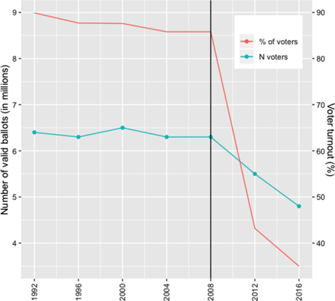
Figure 1. Voter turnout Chilean municipal elections 1992–2016.
From 1990 to 2010, Chile was ruled by the Center-left Nueva Mayoría, coalition that included several left-leaning parties – the Socialist Party, the Party for Democracy, the Radical Party, and the Christian Democracy. This alliance gathered centrist and leftists parties that were at odds before the authoritarian period. Since 2012, the Nueva Mayoría incorporated the Communist Party. The primary challenger of the Nueva Mayoría was the center-right Chile Vamos, which comprised National Renewal, Political Evolution, and the Independent Democratic Union, a rightist party formed initially by close allies of the Pinochet regime. In 2010, Chile Vamos won the presidency, the first time that a right-wing president was democratically elected since 1958.
Chile has 346 municipalities, each of them administered by an elected mayor. Each mayor is elected by a simple majority in single-member districts since 1992, so electoral coalitions are forced to elect one candidate among all the parties to avoid splitting their vote. Although there are a few municipalities with a mayor from a third coalition, the vast majority of mayors are affiliated to one of the two major coalitions. There are no term limits for reelection.
Hypotheses
Following the cited literature, the main hypotheses of this paper are the following:
Hypothesis 1: incumbency advantage was positive in Chile before 2012, because the country has clean and competitive elections. Indeed, previous research in Chile shows that incumbency advantage was positive in congressional elections from 1989 to 2013 (Salas, Reference Salas2016). Thus, both the selection and the sanctioning mechanisms should induce some degree of advantage for office-holders. To test this hypothesis, I estimate the overall incumbency advantage from 1996 to 2008, namely, the years before the adoption of voluntary voting.
Hypothesis 2: after the adoption of voluntary voting, the electorate changed since the cost of voting increased. Per Lijphart (Reference Lijphart1997), the electorate will be more educated and politicized.
Hypothesis 3: in the first election with voluntary voting, incumbency advantage decreases, which may be explained by the following mechanisms:
a. Inefficient campaign spending of long-tenured incumbents. Consider a mayor that was elected several times under mandatory voting. Probably, she has accumulated knowledge on how to run a campaign to maximize their chances. In the first election with voluntary voting, the electorate was unknown for incumbents, since they did not know how voters would react to this new electoral law. Thus, the incumbent mayor may take suboptimal campaign decisions, leading her to, for example, inefficient spending of resources. Another way to put it is that incumbents mayors made fixed investments in campaign technologies that are now obsolete, as their theory of the electorate may be misleading. I will address this hypothesis by analyzing the incumbent’s efficiency in campaign spending in 2008, 2012, and 2016, comparing to the one of challengers. If incumbents have a substantial relative decrease in efficiency levels in 2012, then we can assert that a failure to update the campaign strategy was behind the observed decrease in incumbency levels.
b. Efficient campaign spending of challengers. The adoption of voluntary voting could have induced high-quality challengers to compete for office, since they may have considered that a different electorate gave them a better chance. For instance, they could have anticipated that directing resources to groups that are more likely to vote would increase their chances of succeeding. Thus, high-quality challengers could have been particularly efficient at spending campaign resources. If this is true, we should observe a high correlation between money spent and electoral success.Footnote 3 If the “scaring-off” effect partially explains incumbency (Ashworth and Bueno de Mesquita, Reference Ashworth and Bueno de Mesquita2008; Ban et al., Reference Ban, Llaudet and Snyder2016), more capable challengers will produce a decline in incumbency advantage.
c. The new electorate assigns less weight to incumbency status as a signal of good quality. As Fowler (Reference Fowler2018) argues, voters may perceive incumbency status as a signal of good quality. However, if the electorate is more educated, they may care about other issues rather than incumbency status. If this is true, incumbency advantage should always decrease with a more educated and politicized electorate, so it should be in general low under voluntary voting.
Hypotheses 3a, 3b, and 3c point in the same direction: a decrease in the incumbency advantage in the first election with voluntary voting. However, it is also possible that voluntary voting may increase the incumbency advantage. Under this regime, information about candidates becomes more valuable, giving an edge to candidates with higher name recognition. Or, given that the electorate decreases, perhaps mobilization strategies of office-holders were more decisive than under the old voting regime, giving an extra-advantage to the incumbent. After analyzing different pieces of data, I will discuss which is the most plausible hypothesis and why it is the case that we do not observe an increase in incumbency advantage.
Methods
Incumbency effect
To identify the incumbency advantage, I implemented a RD design for the Chilean case, exploiting the center-left parties margin of victory as the forcing variable (e.g. Lee, Reference Lee2008; Klašnja and Titiunik, Reference Klašnja and Titiunik2017).Footnote 4 Given that at the threshold, the only discontinuous change is the shift on the treatment status – being elected as mayor – it is possible to estimate local average treatment effects (LATE) on the outcomes of interest, in this case, whether the center-left coalition won the next election. Thus, I estimate what is traditionally called the party incumbency, although in this case it should be called the “coalition incumbency,” as I am using the margin of victory of either of the coalition parties. Note that I am estimating this quantity for the years before voluntary voting (1996–2008), to analyze whether incumbency advantage emerges under the same voting regime.
The main RD equation can be written as follows:
 $$wi{n_{it}} = f{\left( X \right)_{it}}_{ - 1} + {\beta _1}{\left( {{X_i} \gt {\rm{ }}{X_0}} \right)_{it}}_{ - 1} + {\rm{ }}e$$
where i represents a municipality in time t. The dependent variable win it indicates if the left candidate won, while f(X)it−1 is a function of the center-left margin forcing variable and (X i > X 0)it−1 is an indicator variable equals to one if the left-wing mayor won the election in time t − 1. The coefficient β 1 represents the treatment effect. For the RD estimation, I use both the optimal bandwidth (Calonico et al., Reference Calonico, Cattaneo and Titiunik2014) and windows of 10, 7.5, and 5 percentage points from the threshold. I also estimate this model with pretreatment covariates at the municipal level (see Table 7 in the appendix for a description of the covariates).
To capture the impact of the adoption of voluntary voting, I follow two analytic strategies. First, I estimate the incumbency effect over time, to see how this quantity changes across different years. Second, I interact the treatment of the RD model with an indicator variable equal to 1 if the election took place in the first year with voluntary voting and 0 if the election happened before 2012. This indicator variable is vol it in equation 2. The interaction term reveals the difference between the incumbency effect of 2012 compared to the years before 2012. This model can be described as follows:
 $$\displaylines{
wi{n_{it}} = {\mkern 1mu} f{\left( X \right)_{it}}_{ - 1} + {\beta _1}{\left( {{X_i} > {X_0}} \right)_{it}}_{ - 1} + {\beta _2}vo{l_{it}} + {\beta _3}\left( {{X_i} > {X_0}} \right)*vo{l_{it}}_{ - 1} + {\beta _4}vo{l_{itit}}_{ - 1} \cr
+ f{\left( X \right)_{it}}_{ - 1} + e \cr} $$
$$\displaylines{
wi{n_{it}} = {\mkern 1mu} f{\left( X \right)_{it}}_{ - 1} + {\beta _1}{\left( {{X_i} > {X_0}} \right)_{it}}_{ - 1} + {\beta _2}vo{l_{it}} + {\beta _3}\left( {{X_i} > {X_0}} \right)*vo{l_{it}}_{ - 1} + {\beta _4}vo{l_{itit}}_{ - 1} \cr
+ f{\left( X \right)_{it}}_{ - 1} + e \cr} $$Here, the coefficient of interest is β 3, which represents the mentioned difference in incumbency advantage. Again, I added covariates to check the robustness of my results.
Note that my empirical strategy does not assume that the adoption of voluntary voting was a random event. As I explained in the previous section, it was intentionally enacted by the main political actors. Instead, I am essentially estimating a heterogeneous incumbency effect in the year of the electoral reform, comparing it to the impact of the years before. Certainly, there may be other aspects that changed in 2012 that may invalidate my analysis. However, after looking at the main electoral reforms in Chile in this period, there are no substantial changes between 2008 and 2012 other than voluntary voting. Indeed, the two main reforms – except the voting regime – happened in 2004 and in 2016. Starting in 2004, municipal legislators were elected in separate elections than mayors, as before that year, legislators were chosen among the candidates for the mayoral office. Moreover, in 2016, a new electoral law created several constraints regarding the source and the amount of campaign funding. Among other things, it forbade corporations to donate to candidates and established a ceiling for the maximum amount of individual donations. In this sense, the main innovation of 2012 compared to 2008 was voluntary voting, as these other reforms happened in different years.
Mechanisms
To capture the change in the electorate, I estimate three linear probability models (LPM), using survey data from 2010, 2012, and 2016. I decided to present the LMP instead of a logistic regression because the quantity of interest is the marginal effect of each independent variable, and the LPM allows us to interpret these effects as the increase in the probability of voting.Footnote 5 Here, I analyze changes in the profile of the likely with voluntary and mandatory voting, by looking at the variables that correlate with voting in the three periods. Needless to say, I am not claiming that such predictors have a causal relationship with voting. This model can be written as follows:
 $$vot{e_i} = \alpha + {\beta ^{'}}{\bf{X}}$$
where vote i is whether the person voted and X is a vector of socioeconomic, demographic, and political variables, including age, years of education, socioeconomic group, self-declared political position, party membership, among others (see Table 9 in appendix for a description of these variables). I also estimate an interacted regression model for 2010 and 2012, including an indicator variable for the period with voluntary voting that is interacted with all the other predictors described in Table 8. A significant interactive effect implies that the correlation of a given predictor and voting changed with voluntary voting. This model can be described as follows:
 $$vot{e_i} = \alpha + {\delta _1}*\, vo{l_{it}} + {\delta _2}^{'}{\bf{X}} + {\beta ^{'}}{\bf{X}}*\,vo{l_{it}}$$
In Table 5, I only show the statistically significant interactive effects of this regression model. I also estimate classification tree models for 2010, 2012, and 2016, to explore patterns in the predictors of voting that may not be captured by the marginal effects. A classification tree segments the predictor space into a number of regions, maximizing predictive accuracy (James et al., Reference James, Witten, Hastie and Tibshirani2013). In this case, this technique allows us to know whether a variable is predictive of voting for specific subgroups of the population. I present a visualization of these classification trees in section “Mechanisms.”
Finally, to test for mechanisms related to campaign spending, I run a linear model to estimate the marginal effect of money spent on the probability of winning. Resources spent are measured in logs of Chilean pesos per person, while the outcome is an indicator variable equal to one if the incumbent (challenger) won and zero otherwise. This simple linear model captures efficiency with regard to the allocation of campaign resources; a positive correlation reveals that more money spent correlates with winning office. In other words, this is a measure of the electoral returns of monetary investment in campaigns. I argue that we can interpret the electoral returns to investment as an indicator of the candidate’s quality. This under the assumption that skilled candidates can a) win office (Ashworth and Bueno de Mesquita, Reference Ashworth and Bueno de Mesquita2008) and b) spend their money efficiently. The equation can be written as follows:
 $$wi{n_{it}} = \alpha + \delta {\left( {log\left( {money} \right)} \right)_{it}}$$
This equation should be interpreted as the marginal effect of 1% of the money spent on the probability of winning office.
Data
This article uses a rich mix of administrative and electoral data. To test the effect of voluntary voting on incumbency, I built a database using data from the Chilean electoral services (SERVEL)Footnote 6 that includes information for party-vote share for the 1992–2016 period, as well as campaign spending for 2008, 2012, and 2016. Continuity tests to check the robustness of the RD estimates were conducted with socioeconomic and demographic data from Chile’s National Institute of Statistics and the Chilean Socioeconomic Household Survey (CASEN).Footnote 7 For the latter survey, I used the versions 2000, 2003, 2006, 2011, and 2015, as these waves include data in most of the municipalities. I also used these sources for the pretreatment covariates of some of the RD models. To characterize the electorate, I use nationally representative survey data of 2010, 2012, and 2016 from the Centro de Estudios Públicos (CEP),Footnote 8 a well-known think-tank that has conducted public opinion polls since the late 1980s.
Results
Descriptive trends
Figure 1 shows trends in voter turnout from 1992 to 1996. When voluntary voting was adopted in 2012, voter turnout substantially decreased, both in absolute numbers and as a percentage of the electorate. Indeed, before 2012, the Chilean electorate was pretty stable, always close to 6.5 million in every election. However, in 2012, only 5.8 million people voted, a million less than in 2008. In this sense, the shock in the electorate was substantive. In 2016, voter turnout decreased even more, reaching only 4.9 million voters. Percentage-wise, the decrease was even larger because, with voluntary voting, there was a large number of eligible voters.
Incumbency advantage
Table 1 shows the overall incumbency advantage for Chile for the period before the adoption of voluntary voting (1996–2008). In general, we observe a positive and substantial incumbency advantage across all specifications, which goes from 0.11 to 0.25 percentage points, depending on the bandwidth. For instance, if we take the most conservative estimate (first column), we see that the effect is 0.11, meaning that barely winners in time t − 1 are 11 percentage points more likely to win in time t. Two of the models are statistically significant at conventional levels, while all the coefficients have the same sign. This suggests that overall, incumbency advantage is positive, as expected by hypothesis 1. Figure 2 shows a visualization of this result.
Table 1. Overall incumbency advantage Chile 1996–2008
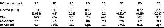
Note: Standard errors in parenthesis. * P-value < 0.1, ** <0.05, *** <0.01. The RD estimate in the last column is bias-corrected with robust variance estimator as described in Calonico et al. (Reference Calonico, Cattaneo and Titiunik2014). The models with covariates only include the period 2000–2008, as the CASEN survey only includes municipal-level data since 2000.
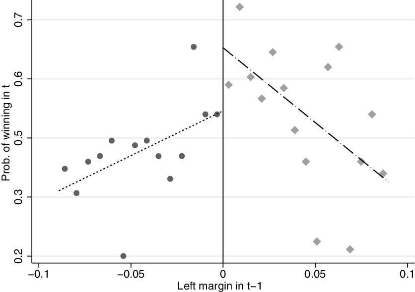
Figure 2. Overall incumbency advantage Chilean mayoral elections 1996–2008.
When analyzing these estimates over time (Table 2), we see that in the first election with incumbent mayors after the return of democracy (1996), the point estimate is practically zero. In the subsequent elections – 2000, 2004, 2008 – we observe a systematic increase of the incumbency advantage, which is also consistent with hypothesis 1. Actually, in 2008, the incumbent had a 39 percentage-point increase in the probability of winning, which is significant at the 0.1 level. However, in 2012, the first year with voluntary voting, the incumbency advantage completely disappears. Interestingly, in 2016, we observe that incumbency advantage reemerges, and its magnitude is even higher than in 2008. This result was somewhat unexpected since in 2016, voter turnout decreased even more. However, this was the second election under the new voting regime, so mayors already had the experience from the past election.
Table 2. Incumbency advantage Chile by year
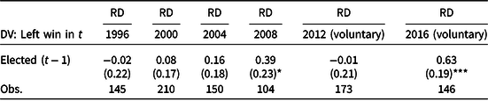
Note: Standard errors in parenthesis. * P-value <0.1, ** < 0.05, *** <0.01. The RD estimates are estimated with an optimal bandwidth, while standard errors are bias-corrected with robust variance estimator as described in Calonico et al. (Reference Calonico, Cattaneo and Titiunik2014).
Table 3 shows the interacted model described in equation 2. The main effect is the incumbency advantage before 2012, while the interaction is the difference in incumbency advantage between 2012 and all the years before. Incumbency advantage in 2012 is the sum of the two coefficients. All the point estimates of the main coefficient are positive, corroborating the results of Table 1. Moreover, the interaction effect is negative in all the models, suggesting that incumbency advantage decreased in 2012. However, there is still some uncertainty in the precision of these results, as in only two of the six models, the estimates of the main coefficient are significant at conventional levels (at least P-value <0.1), while two others have a P-value of less than 0.15. Regarding the interaction term, only one coefficient has a P-value of less than 0.15. Even with this uncertainty – which is mainly explained by lack of statistical power – all the point estimates are consistent with the results in Table 2. Therefore, the evidence suggests that before 2012, incumbency advantage was probably positive, and in 2012, the most likely result is that incumbency decreases.
Table 3. Interacted model incumbency advantage 1996–2012
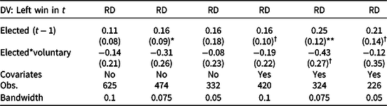
Note: Standard errors in parenthesis. P-value † <0.15, * <0.1, ** <0.05, *** <0.01. The models with covariates only include the period 2000–2008, as the CASEN survey only includes municipal-level data since 2000. I am omitting the constitutive term of voluntary voting, as it is not relevant for the analysis.
Mechanisms
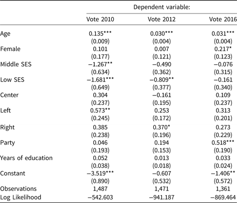
Table 4 shows the profile of the likely voter in mandatory versus voluntary voting for the Chilean case. To capture this profile, I first estimate three LPM models in 2010, 2012, and 2016. Across models, age is an important predictor of voting, although its marginal effect is much larger under compulsory voting (2010). The reader should recall that although voting was mandatory, registration in the electoral records was voluntary. Moreover, being a member of a political party seems to be a relevant predictor in 2016, unlike 2010, and SES was a less relevant predictor in 2016 compared to the other years. For the other variables, we observe a similar marginal effect across the three models. The relevance of age is corroborated in Table 5, since we see that the interaction coefficient between voluntary voting and age is negative and significant, entailing that the importance of age diminished under the new voting regime. None of the other interaction terms are significant (not displayed in the table), corroborating that under voluntary voting, age is a less relevant predictor of voting.
Table 4. Linear probability models Chile 2010, 2012, and 2016 survey data
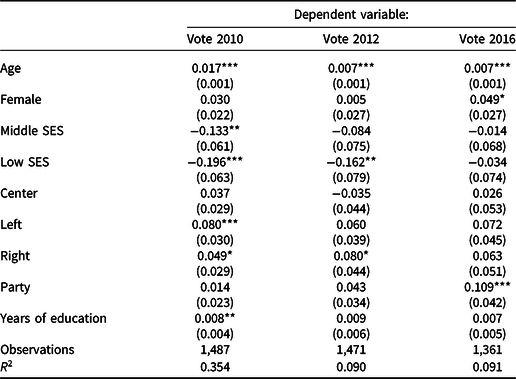
Note: Standard errors in parenthesis. * P-value < 0.1, ** <0.05, *** <0.01. SES refers to socioeconomic status. The reference category for SES is high SES and for political position is no position.
Table 5. Interacted regression model Chile 2010 and 2012 survey data
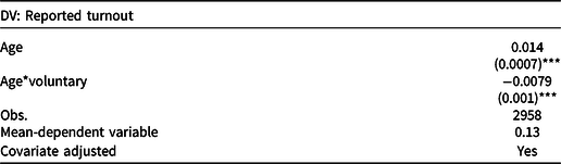
Note: Standard errors in parenthesis. * P-value < 0.1, ** <0.05, *** <0.01.
Figures 3–5 display classification trees for 2010, 2012, and 2016, respectively. Within each box, there is a number between 0 and 1 and a percentage. The number is the predicted probability of each category, while the percentage is the share of observations. For instance, in the bottom right box of Figure 3, the predicted probability of voting for people aged over 39 years 0.94, and 65% of the sample falls in this category. There are two relevant results. First, age became a less relevant predictor of voting under voluntary voting, suggesting that the electorate became younger. Second, in the elections under voluntary voting, there are new relevant predictors among younger people: education in 2012 and political affiliation in 2016.Footnote 9 Thus, under voluntary voting, the electorate became younger, more educated, and politicized, although the characteristics of voters still changed between 2012 and 2016.
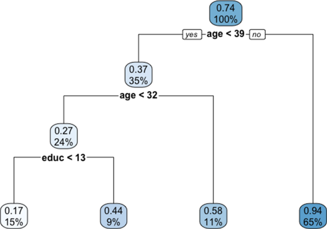
Figure 3. Classification tree mandatory voting Chile 2010.
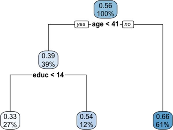
Figure 4. Classification tree voluntary voting Chile 2012.
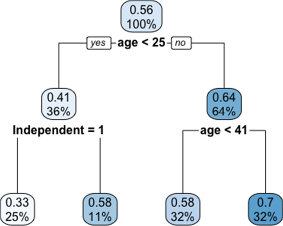
Figure 5. Classification tree voluntary voting Chile 2016.
Overall, both the LPM and the regression trees confirm that the voter’s profile changed under voluntary voting, although we cannot claim that the electorate is substantively more affluent. However, the fact that incumbency advantage reemerged in 2016 rules out a pure voter-centered explanation for the events of 2012. Put in another way, if a smaller and more politicized electorate were the main drivers explaining a general decline of incumbency rates, then we should not observe the reemergence of incumbency in 2016. Thus, it is necessary to look at politicians’ behavior to have a clearer picture of what happened in 2012.
Figures 6–8 show the relationship between campaign spending per person and probability of winning for left-wing candidates, separately for incumbents and challengers. I use this quantity as a measure of efficiency in the allocation of campaign resources. These figures show that in 2008 incumbents are overall more likely to win, and there is a weak and positive relationship between spending and winning for both incumbents and challengers. However, in the first election with voluntary voting (2012), such a relationship remains the same for the incumbent and becomes highly positive for the challenger. This indicates that left-wing challengers were very efficient in spending their campaign resources. Indeed, an additional 1 percent of challenger money spent correlates with an increase of about 22 percentage points on the probability of winning (see Table 10 in the appendix), unlike the previous election. Thus, the 2012 election attracted several high-quality challengers who were able to defeat the incumbents by spending their resources wisely, among other factors. In 2016, the slope for the challenger became less steep, meaning that they did not reach the levels of efficiency of 2012. Thus, left-wing incumbents had almost the same levels of efficiency in campaign spending in the three elections, while challengers substantively increased their efficiency in 2012.
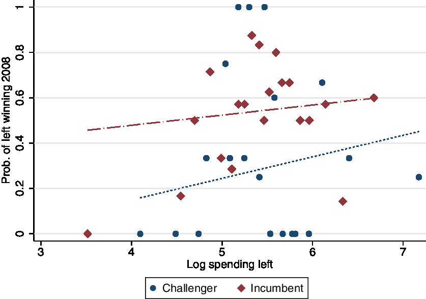
Figure 6. Efficiency in left-wing parties campaign spending left 2008.
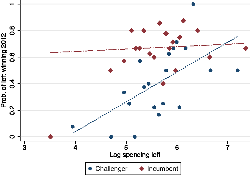
Figure 7. Efficiency in left-wing parties campaign spending left 2012.
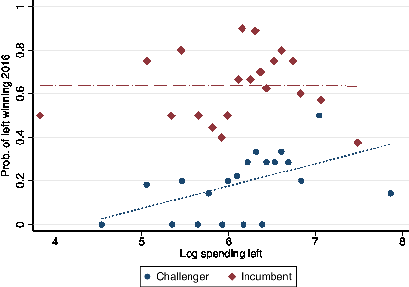
Figure 8. Efficiency in left-wing parties campaign spending left 2016.
For the right, there is a similar trend. In 2008 (Figure 9), both the incumbent and the challenger were fairly efficient at spending campaign resources. However, in 2012, such a relationship remains the same for the incumbent and becomes steeper for the challenger (Figure 10). The slope for the challenger is 0.19, while for the incumbents, it remains at 0.13 (see Table 11 in the appendix). In this sense, right-wing challengers also increased their efficiency in campaign spending in 2012, while incumbents’ efficiency remained constant. In 2016, the challenger’s efficiency clearly declined (Figure 11).
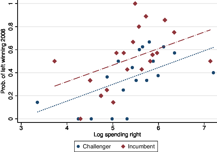
Figure 9. Efficiency in right-wing parties campaign spending 2008.
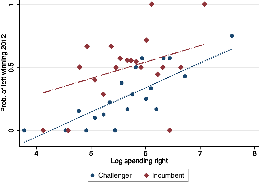
Figure 10. Efficiency in right-wing parties campaign spending 2012.
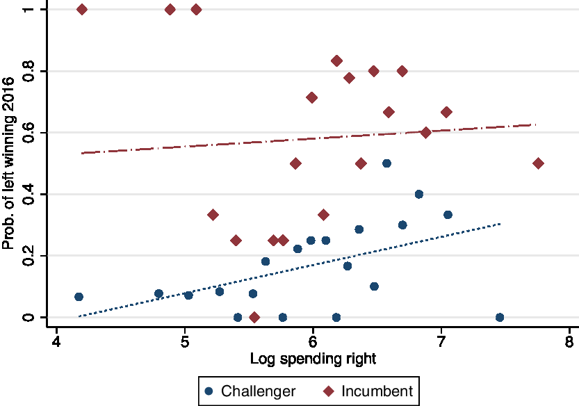
Figure 11. Efficiency in right-wing parties campaign spending 2016.
Overall, this corroborates that the decrease in incumbency advantage was not the result of inefficient campaign spending of incumbents due to voluntary voting, since they were also inefficient before 2012. Most likely, this decrease was the result of the incorporation of high-quality challengers in the electoral competition, as they were able to optimize their resources and defeat the incumbents.
Discussion and conclusion
The evidence presented in this article suggests that shocks in the electorate tend to affect those who are in power. In the Chilean case, we observe that incumbency was positive under compulsory voting, a reasonable outcome in a well-functioning democracy. With the adoption of voluntary voting, the composition of the electorate changed – leading to a smaller, younger and more educated electorate – and incumbency advantage disappeared in 2012, and reemerged in 2016.
I then explore the mechanisms that may explain this decrease in incumbency advantage, finding that in the first election with voluntary voting, challengers were very efficient in their allocation of campaign resources. This suggests that the change in the law encouraged high-quality challengers to compete for office, as they probably perceived that the new conditions – different voting regime and uncertainty in the electorate – could increase their chances of success. Indeed, the evidence indicates that both left and right-wing challengers were skilled enough to spend their money efficiently, as every unit invested yielded high-returns.
In the 2012 election, the main innovation was the adoption of voluntary voting and the shock in the electorate caused by this reform, as in every other aspect, the electoral laws were identical to 2008. For example, candidates in 2012 were subject to the same campaign regulations as in 2008, so it is unlikely that something related to spending explains these results. As described in the hypotheses section, a stricter set of campaign spending regulations were enacted in 2016, the second election with voluntary voting. In this sense, the evidence suggests that efficiency on the spending of high-quality challengers that competed in 2012 is the most plausible explanation of the observed decrease in incumbency advantage, since this phenomenon happened concurrently with the adoption of voluntary voting.
A relevant issue here is the role of the incumbent’s behavior regarding the observed decrease in incumbency advantage. For instance, an important question is: why did not the incumbents, who are aware of the change in electoral rules, adapt their campaign strategies to the new scenario? The evidence provided by the measures of efficiency in campaign spending suggest that incumbents did not decrease their efficiency levels in 2012; indeed, the return for every dollar invested remains constant in 2008, 2012, and 2016. In this sense, there is not enough evidence to sustain hypothesis 3a, namely, that incumbents were particularly inefficient in the first election with voluntary voting. Indeed, it may be true that incumbents were not successful at adapting their strategies for the new electorate, but in light of the evidence, there were not efficient in the past either. Again, what is new is the level of efficiency achieved by challengers, resulting in a substantial decrease in incumbency advantage.
If incumbency levels decreased when high-quality challengers competed for office, then the evidence suggests that in the years before, they decided not to do so. Thus, incumbency advantage was probably affected by a selection-type mechanism: the “scaring-off” effect. Such an effect did not have an impact in 2012, perhaps because high-quality challengers decided to take more risks under a different scenario. However, this wave of capable challengers did not last, as in 2016, incumbency advantage reemerged, and challengers were not particularly efficient at spending their money. Indeed, I cannot discard the possibility that with voluntary voting, electoral behavior is more unpredictable, which may result in higher volatility of electoral outcomes. Although voters’ characteristics may explain a fraction of the effect, I present compelling evidence that a larger share of high-quality challengers competed in the first election with voluntary voting, affecting incumbency effects.
For the theory of electoral accountability, these findings indicate that incumbency advantage emerges as a reasonable outcome in a well-functioning democracy. In the case of Chile, incumbency could have emerged either by the selection of capable politicians (Ashworth and Bueno de Mesquita, Reference Ashworth and Bueno de Mesquita2008; Ban et al., Reference Ban, Llaudet and Snyder2016) or by incentives to perform given the absence of term limits (Klašnja and Titiunik, Reference Klašnja and Titiunik2017). Moreover, we see that institutional reforms that increase the levels of uncertainty in the electoral process produce a temporal shake in the political system. In this sense, even if the reform did not accomplish the goal of inducing a higher number of youngsters to vote, it did help to incorporate a new wave of arguably capable politicians.
In normative terms, I would like to mention three discussions derived from these results. In the first place, the decrease in incumbency advantage per se – at least in one election – may be thought as beneficial, as it introduced new blood in the political system. At the extreme, a system with perfect incumbency would discourage any capable person to compete for office, and it probably would end-up with high levels of corruption. However, a system with no incumbency advantage is also not ideal, since it would probably reflect that electoral accountability is not working as it should. In other words, zero incumbency means that either incumbents do not have incentives to perform or that voters are not willing to reward the incumbent, regardless of performance. In this sense, electoral laws must provide some stability, so incumbents know that it will pay-off to do a good job. For example, in the Chilean case, it is worrisome to observe the steady decline in the voter turnout, since it introduces a level of uncertainty that challenges the core of the idea of electoral accountability.
Second, the higher levels of efficiency achieved by challengers raise the question of how desirable it is for money to have a more significant impact on elections, and if efficiency in the campaign translates to efficiency in public office. The data show that after the adoption of voluntary voting, challengers were more efficient at spending resources during the campaign. In a way, with a smaller electorate, money played a relatively more important role in the election, which ended up giving challengers the edge. This makes perfect sense: with fewer voters, a dollar invested could buy a candidate more votes compared to a situation with a broader electorate. In other words, voluntary voting might have incentives for candidates to spend money on mobilizing core supporters, which may be enough to win the election. In this sense, it would be desirable to also regulate campaign spending, as Chile did in 2016.
Third, I would like to address the normative implications of these findings in light of Lijphart’s argument. Although voter turnout decreased, there is little evidence of a substantial shift toward a more affluent and educated electorate. Yes, under voluntary voting, the electorate became smaller, younger, more educated, and sometimes more politicized. However, it is unclear whether these characteristics will remain stable over time. In this sense, the central phenomenon is that voluntary voting creates uncertainty on the composition of the electorate in each election. The whole range of political consequences of this phenomenon remains to be seen.
Appendix A. Additional tables
Table 6. Continuity tests
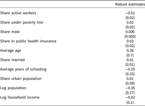
Note: Standard errors in parenthesis. * P-value < 0.1, ** < 0.05, *** < 0.01. The estimates are bias-corrected with robust variance estimator as described in Calonico, Cattaneo and Titiunik (Reference Calonico, Cattaneo and Titiunik2014).
Table 7. Description of pretreatment covariates used in the RD models
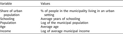
Table 8. Logistic regression models Chile 2010, 2012 and 2016
Note: Coefficients are in log-odds. Standard errors in parenthesis. * P-value < 0.1, ** < 0.05, *** < 0.01. SES refers to socioeconomic status. The reference category for SES is high SES and for political position is no position.
Table 9. Description of CEP variables
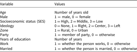
Table 10. Linear model of probability of winning on campaign spending (left-wing parties)
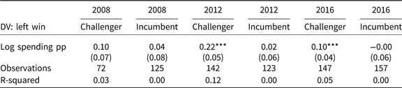
Note: Standard errors in parentheses.
*** P < 0.01, ** P < 0.05, * P < 0.1
Table 11. Linear model of probability of winning on campaign spending (right-wing parties)
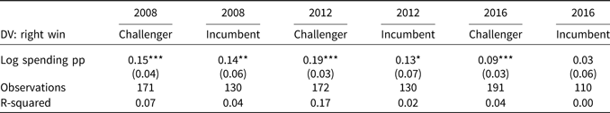
Note: Standard errors in parentheses.
*** P < 0.01, ** P < 0.05, * P < 0.1
Appendix B. The Netherlands case
As a complementary case, I provide correlational evidence of the effect of voluntary voting on incumbency in the Netherlands, country that adopted voluntary voting in the parliamentary election of 1970. In this case, I use a difference-in-difference model, using Belgium as a counterfactual, that is, as a similar case that did not implement such electoral reform. Following Miller and Dassonmeville’s (Reference Miller and Dassonneville2016), Belgium is a good comparison because it is a neighbor country that shares several features with the Netherlands, such as the language, the electoral system, party systems, among other elements.
Background
In 1917, the Netherlands adopted both a PR electoral system and a mandatory voting regime. In the 40 s, Dutch politics was dominated by the Catholic’s People Party and the Labour Party. The former is a center-right confessional party, which was the continuation of the General League of Roman Catholic Caucuses. From 1946 to 1972, they participated in a government coalition in every single period, so it is safe to denominate this party as the leading incumbent. The Labour party emerged from the union of the Social Democratic Worker’s party, the Free Thinking Democratic League, and the Christian Democratic Union in 1946. This party belonged to the government coalition from 1946 to 1956, while in the 1956–1972 period, they were mostly in the opposition. By the 60 s, the notion that citizens should decide whether to attend to the polls or not was increasingly popular, leading to the abolition of compulsory voting for the 1970 election (Miller and Dassonneville, Reference Miller and Dassonneville2016).
In Belgium, the Christian Social Party existed between 1946 and 1968, and it belonged to the Government Coalition in a majority of periods. In 1968, the party divided along linguistic lines, creating the Christian Social Party in Wallonia and the Christian People’s Party in Flanders. The Belgian Socialist Party was founded in 1945, and it was the primary challenger of the Catholic party. Belgium did not change its voting regime, maintaining compulsory voting until today.
Data and methods
I use the data from Miller and Dassonmeville’s (Reference Miller and Dassonneville2016) paper on the adoption of voluntary voting in the Nether-lands, a provincial-level data set from 1946 to 2014, which includes party vote share variables and several demographic covariates. These data were kindly facilitated to me directly by the authors.Footnote 10 As Miller and Dassonneville (Reference Miller and Dassonneville2016), I use the party categorization ParlGov to define parties as either Catholic or Laborist. ParlGov is a database of European and OECD countries built by the Center for Social Policy Research at the University of Bremen (Doring and Manow, Reference Doring and Manow2015). For the models presented in Table 12, I used data from 1960 to 1980, to avoid having data points too far away from the treatment.
I implement a difference-in-difference model, using the adoption of voluntary voting as the treatment and Belgium as the counterfactual case, following a similar strategy as Miller and Dassonneville (Reference Miller and Dassonneville2016). However, the difference is that I focus on incumbent vote share as the main dependent variable, while their focus is on leftist parties vote share. Given that the country has a proportional representation system, and due to data constraints, I was only able to get data on parliamentary elections. In this sense, the identification strategy of this section is less robust compared to the Chilean case. The main equation can be written as follows:
 $$v{s_{it}} = \alpha + {\beta _1}{\left( {vol} \right)_{it}} + {\delta _i} + {\gamma _t} + {\beta _2}{\left( {dem} \right)_{it}} + e$$
where vs it is the incumbent vote share at district i in time t, vol is an indicator variable for the adoption of voluntary voting, δ i and γ t are district and time fixed effects, and dem it is a vector of demographics controls, which includes the log the number of eligible voters and GDP growth the year before the election. At that time, the incumbent in the Netherlands was the Catholic’s People Party, so I use the vote share of this party as a proxy for incumbent’s vote share. I also used Labour party vote share as the outcome to test if voluntary voting correlates with an increase of left-of-center parties (see Table 12). Given that this is a proportional system, I am defining incumbency as the correlation between the adoption of voluntary voting and national incumbent vote share in the Netherlands compared to such correlation in Belgium.
Results
Figure 12 shows trends in voter turnout for the Netherlands case. We a large observe a decline in voter turnout after 1967, both percentage-wise in absolute numbers. Indeed, there is a decline of more than 1 million votes, higher than any other absolute decline in voter turnout.
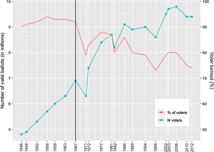
Figure 12. Voter turnout in Netherlands parliamentary elections 1946–2012.
Figure 13 shows the trends of the Catholic Party in Belgium and the Netherlands,Footnote 11 the majority parties of their respective countries. We see that immediately after the adoption of voluntary voting (1970), there is a large decrease in the Netherlands Catholic Party vote share, from 45% to 37%. However, in Belgium – country which maintained compulsory voting – we do not observe such a decrease. In Miller and Dassonneville’s (Reference Miller and Dassonneville2016) paper, this decrease is also documented, although it is interpreted in a different way. According to their hypothesis, the adoption of voluntary voting benefits left-of-center parties, while I am focusing on the implications for incumbents’ vote share.
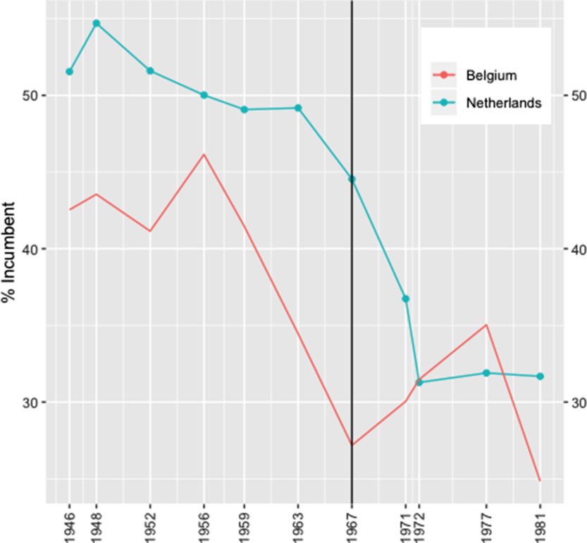
Figure 13. Incumbent party vote share in Netherlands and Belgium.
Is this effect explained by a decline of the incumbent or by a boost of the left? Table 12 shows a province-level fixed effect model, using both incumbent and Social Democratic party vote share as the dependent variables, for both the Netherlands and Belgium. When looking at the first two columns, we see that the effect of voluntary voting on the incumbent’s vote share is consistently negative. Indeed, in the adjusted models, the result looks even more significant. When looking at the models with social democratic vote share as the dependent variable, we see that the effect of voluntary voting is positive in the nonadjusted model, but it disappears when adjusting for demographic variables. In this sense, the evidence suggests that the incumbent was harmed by such reform, while the effect on center-left parties is less clear. This finding goes in the same direction as the results for Chile in 2012.
Table 12. Fixed-effects models Netherlands 1960–1980
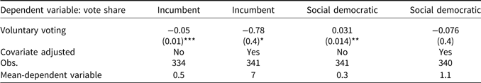
Standard errors in parenthesis. * P-value < 0.1, ** < 0.05, *** < 0.01. Standard errors are clustered at the province level. The RD estimates are bias-corrected with robust variance estimator as described in Calonico et al. (Reference Calonico, Cattaneo and Titiunik2014).


