


1. Introduction
In terms of value, wine is the most traded agricultural product between the United States (US) and the European Union (EU)Footnote 1 (US Department of Agriculture Foreign Agricultural Service, 2020). The US imported 3.9 billion USD (US dollars) worth of wine from the EU in 2015, while the EU member states imported 618 million USD of wine from the US. According to the Wine Institute (2019), Americans have increased their total wine consumption from 449 million gallons in 1993 (1.74 gallons per resident) to 966 million gallons in 2018 (2.95 gallons per resident). Of the 70.5 billion USD Americans spent on wine in 2018, domestic wines (mainly from California) accounted for approximately 67% (47.2 billion USD), while 33% (23.3 billion USD) was spent on imported wines (Wines Vines Analytics, 2019). Of all the wine consumed in the US in 2017, red wines made up 42% of the wine consumed, while white wines made up 33% (Wine Market Council, 2019).
The US and the EU both have a variety of domestic and international policies in place that affect wine trade, including schedules of differentiated tariffs and a variety of non-tariff barriers set through domestic regulations. In this article, we evaluate the welfare effects of the October 2019 Section 301 tariffs imposed by the Trump administration on certain EU wines (84, Fed. Reg. October 9, 2019, 54245–54264) in response to EU subsidies on Airbus production. An additional 25% tariffs are applied to wines imported into the US from France, Germany, Spain, and the United Kingdom (UK). As such, the effects of the newly imposed additional wine tariffs are differential in that wines from other countries, including other EU countries, are exempt from the tariff increase.
The purpose of the paper is to quantify the impacts of the October 2019 US tariff increases on US importers of both red wines and white wines sourced from various exporting countries. To do so, we analyze US import demand for both red and white wines by individual source countries. In particular, this allows us to capture varying consumer preferences for red wine imports versus white wine imports. We estimate own- and cross-price elasticities and use these elasticities to analyze the quantity, revenue, and welfare effects of the October 2019 EU wine tariff increases that stemmed from a long-standing trade dispute between the US and the EU.
The rest of the paper is organized as follows. We first review the trade disputes between the US and the EU that led to the additional 25% tariffs on US imports of certain EU wines in October 2019. Then, we introduce the conceptual framework for estimating source-differentiated import demand systems for imported red and white wines. Following that, we summarize the data and present the relevant price and expenditure elasticities of import demand for red and white wines by source countries. Next, we simulate the welfare effects of a 25% tariff on red and white wine imports from certain EU countries on US wine importers as well as tariff-imposed and no-tariff-imposed exporters of wine. We conclude by highlighting the important findings of our analysis.
2. US Wine Imports and Recent Trade Disputes with the EU
Trade tensions between the US and the EU that ultimately led to the recent Section 301 tariffs on some EU wines started in 2006 when the US filed a case with the World Trade Organization (WTO) against the EU for the subsidies it provided to Airbus. In what follows, we provide historical developments that led to the additional 25% wine tariffs imposed by the Trump administration in October 2019 on certain EU wines.
In March 2018, the Trump administration announced 25% steel and 10% aluminum tariffs on most US trading partners (including the EU), citing an April 2017 investigation under Section 232 of the 1962 Trade Expansion Act, which concluded that these steel and aluminum imports could weaken US national security. The EU has viewed the US national security justification for steel and aluminum tariffs as groundless and inconsistent with the WTO rules. In June 2018, the EU started implementing retaliatory tariffs of 25% on imports of some US agricultural goods (whisky, corn, rice, kidney beans, preserved and mixed vegetables, orange juice, cranberry juice, peanut butter, and tobacco products, totaling 1.2 billion USD in 2018) along with select non-agricultural products (CRS, February 27, 2020, p. 6). In January 2019, The Office of the US Trade Representative (USTR) announced that it would enter formal trade negotiations with the EU to resolve disputes regarding market access and non-tariff measures, including those affecting agricultural products. However, the April 2019 negotiating mandate announced by the EU excluded agricultural products from trade talks with the US.
Trade disputes between the EU and the US escalated in October 2019 when the US imposed further tariffs on 7.5 billion USD worth of US imports from the EU, citing the Section 301 enforcement of the US WTO Rights in Large Civil Aircraft Dispute (84, Fed. Reg. October 9, 2019, 54245–54264). These tariffs were based on a 16-year long dispute and litigation between the US and the EU regarding their domestic aircraft industry (Boeing in the US, and Airbus in the EU). Both sides claimed that the other side’s airplane manufacturer was being unfairly subsidized. The US was the first to file a case with the WTO in 2006, claiming that Airbus, a multinational company jointly owned by Germany, France, Spain, and the United Kingdom, had received 22 billion USD in illegal subsidies. The EU put forward a counter case against the US, claiming that Boeing had received 23 billion USD in trade-distorting domestic subsidies for its research and development projects. In 2018, the WTO’s appeals body upheld a 2016 ruling that the EU had illegally assisted Airbus with subsidized loans for the development of new aircraft. In its final ruling on the US case against Airbus, on October 2, 2019, the WTO allowed the US to impose tariffs on up to 7.5 billion USD worth of EU goods (CRS, August 25, 2020).
The US administration’s choice of EU products for the new tariffs was broad. In October 2019, the USTR published a list of 158 products subject to additional duties (84, Fed. Reg. October 9, 2019, 54245–54264). The list targeted mainly US imports from France, Germany, Spain, and the United Kingdom but was not limited to the aircraft industry. While the tariffs on large civil aircraft—the subject of the original dispute—were increased by only 10%, some agricultural and related consumer-oriented products from the EU were hit by a 25% increase in tariffs. Wine was one of the main EU imports taxed at an additional 25% tariff after October 18, 2019. Prior to the October 2019 tariffs, the average tariff on EU wine imports was only 0.7% (CRS, August 25, 2020). Wines from the EU made up about 17% of the 7.5 billion USD worth of EU imports targeted by the October 2019 tariffs (CRS, February 2020, p. 9). Other agricultural and related products affected included whiskies and liquors, cheese and dairy, olives and olive products, pork and pork products, biscuits, wafers, fruits, and fruit products.
The USTR reevaluates the tariff actions periodically based on the progression of trade negotiations with the EU. With their August 2020 review, the USTR decided to maintain the 25% additional tariffs imposed in October 2019 on EU wines (and, almost all other goods) and left the possibility of higher future tariffs open. An important question raised by these recent tariffs on EU wines is how the additional 25% tariffs affect the US wine importers as well as gains of the non-tariff countries exporting wine into the US. In what follows, we use a source-differentiated import demand model for imported red and white wines to simulate the welfare effects of these wine tariffs imposed on specific EU countries.
3. A Source-Differentiated Differential Demand Model for Imported Wines
The empirical literature on demand for alcoholic beverages, including wine, is well established. However, a significant strand of the previous research focuses on aggregate wine demand in comparison to the demand for other alcoholic products, such as beer and spirits (e.g., Andrikopoulos, Brox, and Carvalho, Reference Andrikopoulos, Brox and Carvalho1997; Andrikopoulos and Loizides, Reference Andrikopoulos and Loizides2000; Chang, Griffith, and Bettington, Reference Chang, Griffith and Bettington2002; Gao, Wailes, and Cramer, Reference Gao, Wailes and Cramer1995; Levi and Folwell, Reference Levi and Folwell1995; Salisu and Balasubramanyam, Reference Salisu and Balasubramanyam1997; Selvanathan, Reference Selvanathan1991; Tsolakis, Riethmuller, and Watts, Reference Tsolakis, Riethmuller and Watts1983). Since Armington’s (Reference Armington1969) seminal study that differentiated internationally traded products based on the geographical origin of the products, a few studies have estimated source-differentiated demand systems for imported wines, such as Muhammad (Reference Muhammad2011) for UK wine imports, and Muhammad et al. (Reference Muhammad, Leister, McPhail and Chen2014); Agnoli, Capitello, and Begalli (Reference Agnoli, Capitello and Begalli2014); Capitello, Agnoli, and Begalli (Reference Capitello, Agnoli and Begalli2015); and Muhammad and Countryman (Reference Muhammad and Countryman2019) for Chinese wine imports. The aforementioned studies have not distinguished imported wines by their color. We are aware of only three studies estimating a source-differentiated import demand model for a particular color of wine: Seale, Marchant, and Basso (Reference Seale, Marchant and Basso2003) for US red wine imports; Carew, Florkowski, and He (Reference Carew, Florkowski and He2004) for British Columbian red and white wine imports from the EU and the US; and Lee, Kennedy, and Hilbun (Reference Lee, Kennedy and Hilbun2009) for Korean red wine imports.
Our analysis of recent increases in US tariffs on wines from certain EU nations is based on an import demand model of wine by country of origin, where the same type of wine (i.e., red, white, and other wines of fresh grapes) from different exporting countries is treated as different products by US consumers. We use a multistage budgeting or the utility tree approach (Barten, Reference Barten1977), where an importing country first allocates total expenditure between domestic goods and imported goods. In stage 2, total import expenditure is allocated among imported groups of goods such as imported wine that includes red, white, and other wines. In the next stage, total import expenditure for group g, in our case wine, is allocated among the different types of wines (i.e., red, white, and other wines) and finally total import expenditure for good i, say red wine, is allocated among red wine by source country (e.g., Seale, Sparks, and Buxton, Reference Seale, Sparks and Buxton1992). We maintain weak separability between domestic and imported goods (e.g., Muhammad et al., Reference Muhammad, Leister, McPhail and Chen2014; Muhammad and Countryman, Reference Muhammad and Countryman2019) due to the lack of data on domestic red and white wine prices. To our knowledge, the only study that uses US domestic price data in a disaggregated, source-differentiated red wine demand model is Seale, Marchant, and Basso (Reference Seale, Marchant and Basso2003), who utilized their connections with a private consulting firm to obtain the proprietary price data (Seale, Marchant, and Basso, Reference Seale, Marchant and Basso2003, p. 190).
Following Schmitz and Seale (Reference Schmitz and Seale2002); Asci et al. (Reference Asci, Seale, Onel and VanSickle2016); and Zhang and Seale (Reference Zhang, Seale, Schmitz, Kennedy and Schmitz2017), our empirical strategy starts with choosing the best-fitting functional form among a family of differential demand systems (i.e., Rotterdam [Theil, Reference Theil1965], CBS [Keller and van Driel, Reference Keller and Van Driel1985], differential AIDS [Deaton and Muellbauer, Reference Deaton and Muellbauer1980], and NBR [Neves, Reference Neves1987]), each with a different functional form. The functional form developed by Lee, Brown, and Seale (Reference Lee, Brown and Seale1994) (LBS) extends an earlier functional form by Barten (Reference Barten1993) to nest other four differential demand systems presented below. Therefore, we start our empirical analysis with the LBS model:
 $$$\;\;\;\;\;{w_i}d\left( {{\rm{ln}}{q_i}} \right) = \left( {{\delta _1}{w_i} + {d_i}} \right)d\left( {{\rm{ln}}Q} \right) + \mathop \sum \limits_j [{e_{ij}} - {\delta _2}{w_i}\left( {{\delta _{ij}} - {w_j}} \right)]d({\rm{ln}}{p_j}) + {\varepsilon _i},$$$
where  ${d_i} = {\delta _1}{\beta _i} + \left( {1 - {\delta _1}} \right){\theta _i}$
,
${d_i} = {\delta _1}{\beta _i} + \left( {1 - {\delta _1}} \right){\theta _i}$
,  ${e_{ij}} = {\delta _2}{\gamma _{ij}} + \left( {1 - {\delta _2}} \right){\pi _{ij}}$
, and
${e_{ij}} = {\delta _2}{\gamma _{ij}} + \left( {1 - {\delta _2}} \right){\pi _{ij}}$
, and  ${\delta _1}{\rm{ and }}\ {\delta _2}{\rm{ }}$
are two additional nesting parameters to be estimated;
${\delta _1}{\rm{ and }}\ {\delta _2}{\rm{ }}$
are two additional nesting parameters to be estimated;  ${\pi _{ij}}$
is a compensated (Slutsky) price parameter for commodity
${\pi _{ij}}$
is a compensated (Slutsky) price parameter for commodity  $i$
with respect to the price of commodity
$i$
with respect to the price of commodity  $j$
;
$j$
;  ${\gamma _{ij}} = {\pi _{ij}} + {w_i}\left( {{\delta _{ij}} - {w_j}} \right)$
;
${\gamma _{ij}} = {\pi _{ij}} + {w_i}\left( {{\delta _{ij}} - {w_j}} \right)$
;  ${\delta _{ij}}$
is the Kronecker delta equal to one when
${\delta _{ij}}$
is the Kronecker delta equal to one when  $i = j$
and zero otherwise;
$i = j$
and zero otherwise;  ${w_i} = {p_i}{q_i}/\mathop \sum \limits_{i = 1}^n {p_i}{q_{i\;\;\;}}$
represents the budget share of good
${w_i} = {p_i}{q_i}/\mathop \sum \limits_{i = 1}^n {p_i}{q_{i\;\;\;}}$
represents the budget share of good  $i$
(i = 1,…, n) with n representing the number of goods;
$i$
(i = 1,…, n) with n representing the number of goods;  ${\rm{ln}}{q_i}$
and
${\rm{ln}}{q_i}$
and  ${\rm{ln}}{p_j}$
are the natural logs of the quantity of good
${\rm{ln}}{p_j}$
are the natural logs of the quantity of good  $i$
and the price of good
$i$
and the price of good  $j$
, respectively, while
$j$
, respectively, while  ${\theta _i}$
is
${\theta _i}$
is  ${{\partial \left( {{p_i}{q_i}} \right)} \over {\partial M}}$
, which is defined as the marginal share; and
${{\partial \left( {{p_i}{q_i}} \right)} \over {\partial M}}$
, which is defined as the marginal share; and  $d\left( {{\rm{ln}}Q} \right) = \mathop \sum \limits_{i = 1}^n {w_i}d\left( {{\rm{ln}}{q_i}} \right)$
is the Divisia volume index that represents real expenditure.
$d\left( {{\rm{ln}}Q} \right) = \mathop \sum \limits_{i = 1}^n {w_i}d\left( {{\rm{ln}}{q_i}} \right)$
is the Divisia volume index that represents real expenditure.
The LBS maintains adding-up restrictions, while homogeneity and symmetry can be imposed:
Adding-up:  $\;\mathop \sum \limits_i {d_i} = 1 - {\delta _1}$
and
$\;\mathop \sum \limits_i {d_i} = 1 - {\delta _1}$
and  $\mathop \sum \limits_i {e_{ij}} = 0$
,
$\mathop \sum \limits_i {e_{ij}} = 0$
,
Homogeneity:  $\;\mathop \sum \limits_j {e_{ij}} = 0$
, and
$\;\mathop \sum \limits_j {e_{ij}} = 0$
, and
Symmetry:  ${e_{ij}} = {e_{ji}}$
.
${e_{ij}} = {e_{ji}}$
.
Using the LBS functional form that nests Rotterdam, differential AIDS, CBS, and NBR functional forms, one can test for the functional form that best fits the data. In addition, if selected as the best-fitting model against the alternatives, the LBS model is also a theoretically consistent demand model in its own right (Asci et al., Reference Asci, Seale, Onel and VanSickle2016; Barten, Reference Barten1993; Lee, Brown, and Seale, Reference Lee, Brown and Seale1994; Matsuda, Reference Matsuda2005). By placing particular restrictions on the  ${\delta _1}$
and
${\delta _1}$
and  ${\delta _2}$
parameters, LBS yields the four other functional forms considered for the empirical specification.
${\delta _2}$
parameters, LBS yields the four other functional forms considered for the empirical specification.
Rotterdam (Theil, Reference Theil1965):  ${\delta _1} = 0{\rm{\;}}$
and
${\delta _1} = 0{\rm{\;}}$
and  ${\delta _2} = 0$
,
${\delta _2} = 0$
,
 $$${w_i}d\left( {{\rm{ln}}{q_i}} \right) = {\theta _i}d\left( {{\rm{ln}}Q} \right) + \mathop \sum \limits_{j = 1}^n {\pi _{ij}}d({\rm{ln}}{p_j});$$$
CBS (Keller and van Driel, Reference Keller and Van Driel1985):  ${\delta _1} = 1{\rm{\;}}$
and
${\delta _1} = 1{\rm{\;}}$
and  ${\delta _2} = 0$
,
${\delta _2} = 0$
,
 $$${w_i}d\left( {{\rm{ln}}{q_i}} \right) = \left( {{\beta _i} + {w_i}} \right)d\left( {{\rm{ln}}Q} \right) + \mathop \sum \limits_{j = 1}^n {\pi _{ij}}d({\rm{ln}}{p_j}) + {\varepsilon _i};$$$
Differential AIDS (Deaton and Muellbauer, Reference Deaton and Muellbauer1980):  ${\delta _1} = 1{\rm{\;}}$
and
${\delta _1} = 1{\rm{\;}}$
and  ${\delta _2} = 1$
,
${\delta _2} = 1$
,
 $$$\;{w_i}d\left( {{\rm{ln}}{q_i}} \right) = \left( {{\beta _i} + {w_i}} \right)d\left( {{\rm{ln}}Q} \right) + \mathop \sum \limits_j [{\gamma _{ij}} - {w_i}\left( {{\delta _{ij}} - {w_j}} \right)]d\left( {{\rm{ln}}{p_j}} \right) + {\varepsilon _i};$$$
and, NBR (Neves, Reference Neves1987):  ${\delta _1} = 0{\rm{\;}}$
and
${\delta _1} = 0{\rm{\;}}$
and  ${\delta _2} = 1$
,
${\delta _2} = 1$
,
 $$$\;{w_i}d\left( {{\rm{ln}}{q_i}} \right) = \left( {{\beta _i} + {w_i}} \right)d\left( {{\rm{ln}}Q} \right) + \mathop \sum \limits_j [{\gamma _{ij}} - {w_i}\left( {{\delta _{ij}} - {w_j}} \right)]d\left( {{\rm{ln}}{p_j}} \right) + {\varepsilon _i}.$$$
To operationalize the functional forms for estimation purposes, we replace  ${w_i}$
with its arithmetic mean
${w_i}$
with its arithmetic mean  $\left( {{w_i} = \left( {{w_{i,t}} + {w_{i,t - 1}}} \right)/2} \right)$
and use
$\left( {{w_i} = \left( {{w_{i,t}} + {w_{i,t - 1}}} \right)/2} \right)$
and use  $d\left( {{\rm{ln}}X} \right) = {\rm{ln}}{X_t} - {\rm{ln}}{X_{t - 1}}$
, where X represents
$d\left( {{\rm{ln}}X} \right) = {\rm{ln}}{X_t} - {\rm{ln}}{X_{t - 1}}$
, where X represents  $p$
and
$p$
and  $q$
.
$q$
.
Initially, we estimate group demand for imported wine (i.e., red, white, and other wines) and find that the differential AIDS, without a trend variable and corrected for autocorrelation, best fits the grouped data. Let i (1,…,n) represent wine by source country and let the n wines by source country be divided among G < n groups, written  ${S_1}, \ldots ,{S_G},$
with each good belonging to exactly one group. Let
${S_1}, \ldots ,{S_G},$
with each good belonging to exactly one group. Let  $i \in {S_g}$
represent good i contained in group
$i \in {S_g}$
represent good i contained in group  ${S_g}$
,
${S_g}$
,  $j \in {S_h}$
represent good j contained in group
$j \in {S_h}$
represent good j contained in group ${S_h}$
, and let h represent other groups,
${S_h}$
, and let h represent other groups,  $g \ne h$
. Let these G groups of goods be blockwise dependent such that the utility function is an increasing function of the group utility functions,
$g \ne h$
. Let these G groups of goods be blockwise dependent such that the utility function is an increasing function of the group utility functions,  $u(q) = f\left( {{u_1}\left( {q_1^*} \right),\ldots,{u_G}\left( {q_G^*} \right)} \right)$
where
$u(q) = f\left( {{u_1}\left( {q_1^*} \right),\ldots,{u_G}\left( {q_G^*} \right)} \right)$
where  $q_g^*$
represents the vector of
$q_g^*$
represents the vector of  ${q_i}$
’s in group
${q_i}$
’s in group  ${S_g}$
within the imported wine group. Then, the group demand can be illustrated as follows using, say, the differential AIDS functional form:
${S_g}$
within the imported wine group. Then, the group demand can be illustrated as follows using, say, the differential AIDS functional form:
 $$${W_g}d\left( {\ln {Q_g}} \right) = \left( {{W_g} + {{\rm B}_g}} \right)d\left( {{\rm{ln}}Q} \right) + \sum\limits_{h = 1}^G {\left[ {{\Gamma _{gh}} - {W_g}\left( {{\delta _{gh}} - {W_h}} \right)} \right]d\left( {{\rm{ln}}{P_h}} \right)} + {\varepsilon _{gh}},$$$
where  ${W_g} = \sum\nolimits_{i \in {s_g}} {w_i^*} $
is the group budget share for group
${W_g} = \sum\nolimits_{i \in {s_g}} {w_i^*} $
is the group budget share for group  ${S_g}$
and
${S_g}$
and  $w_i^* = {{{w_i}} \over {{W_g}}}$
is the conditional budget share of good
$w_i^* = {{{w_i}} \over {{W_g}}}$
is the conditional budget share of good  $i \in {S_g}$
;
$i \in {S_g}$
;  ${P_h}$
is the price of group
${P_h}$
is the price of group  ${S_h}$
;
${S_h}$
;  $d\left( {{\rm{ln}}{Q_g}} \right)$
is the Divisia volume index for group
$d\left( {{\rm{ln}}{Q_g}} \right)$
is the Divisia volume index for group  ${S_g}$
to be defined below after equation (7); and
${S_g}$
to be defined below after equation (7); and  ${{\rm B}_g}$
and
${{\rm B}_g}$
and  ${\Gamma _{gh}}$
are constant parameters to estimate.
${\Gamma _{gh}}$
are constant parameters to estimate.
The conditional demand for source-specific imported good  $i$
contained in group
$i$
contained in group  ${S_g}$
, using the LBS functional form for illustrative purposes, is
${S_g}$
, using the LBS functional form for illustrative purposes, is
 $$$\;\;\;\;\;w_i^*d\left( {{\rm{ln}}{q_i}} \right) = \left( {{\delta _1}w_i^* + d_i^*} \right)d\left( {{\rm{ln}}{Q_g}} \right) + \mathop \sum \limits_{j \in g} [e_j^* - {\delta _2}w_i^*\left( {{\delta _{ij}} - w_j^*} \right)]d\left( {{\rm{ln}}{p_j}} \right) + {\varepsilon _i}$$$
where  $w_i^* = {{{w_i}} \over {{W_g}}}$
,
$w_i^* = {{{w_i}} \over {{W_g}}}$
,  $d\left( {{\rm{ln}}{Q_g}} \right) = \sum\nolimits_{i \in {S_g}} {w_i^*d\left( {\ln {q_i}} \right)} $
, and
$d\left( {{\rm{ln}}{Q_g}} \right) = \sum\nolimits_{i \in {S_g}} {w_i^*d\left( {\ln {q_i}} \right)} $
, and  $d_i^*$
,
$d_i^*$
,  $e_{ij}^*$
,
$e_{ij}^*$
,  ${\delta _1}{\rm{\;}}$
, and
${\delta _1}{\rm{\;}}$
, and  ${\delta _2}$
are constant parameters to estimate. Empirical results presented in the next section suggest that the LBS model is selected for source-differentiated red and white wine imports. We present conditional and unconditional elasticity formulae for selected models in Appendix B, Table B1. In calculating unconditional elasticities, we use parameters from both the first-stage group demand and the second-stage source-differentiated demand and derive the formulae in Table B1 using the theory of group demand and conditional demand with the differential approach to consumer demand (Theil, Reference Theil1980). Theoretical restrictions and model specification tests are conducted using Likelihood Ratio tests, which follow a
${\delta _2}$
are constant parameters to estimate. Empirical results presented in the next section suggest that the LBS model is selected for source-differentiated red and white wine imports. We present conditional and unconditional elasticity formulae for selected models in Appendix B, Table B1. In calculating unconditional elasticities, we use parameters from both the first-stage group demand and the second-stage source-differentiated demand and derive the formulae in Table B1 using the theory of group demand and conditional demand with the differential approach to consumer demand (Theil, Reference Theil1980). Theoretical restrictions and model specification tests are conducted using Likelihood Ratio tests, which follow a  ${\chi ^2}\left( q \right)$
distribution, where
${\chi ^2}\left( q \right)$
distribution, where  $q$
represents the number of restrictions imposed.
$q$
represents the number of restrictions imposed.
4. Estimation Results
4.1. Data
Data on US red wine and white wine imports by exporting country were obtained from the Global Agricultural Trade System of the US Department of Agriculture, Foreign Agricultural Service (USDA-FAS, 2020). Monthly import data from January 1990 to October 2019 were composed of wines of fresh grapes classified under the Harmonized Commodity Description and Coding System at the ten-digit level, providing a sample size of 358 observations. The initial part of the analysis categorizes fresh grape wines under red, white, and other fresh grape wine. The category other wines of fresh grapes includes sparkling wine, effervescent wine, and other fortified grape wine varieties. In order to keep the source-differentiated demand systems at manageable sizes, we do not disaggregate each color wine further into dry, semi-sweet, and sweet varieties. For the source-differentiated demand analysis of red and white wines, we include data for the top five exporting countries ranked by the value of their wine exports to the US within the sample period. Remaining countries exporting red and white wines to the US were classified as the Rest of the World (ROW). Accordingly, major source countries for US imported red wine were identified as France, Italy, Chile, Spain, Australia, and the ROW; the major source countries for US imported white wine were identified as France, Italy, Australia, New Zealand, Germany, and the ROW. Footnote 2 Unit prices of wine were derived by dividing value of imports (thousand USD) by quantity of imports (thousand gallons). Analyses are conducted on a per capita basis using US population data obtained from the US Census Bureau (2020).
Descriptive statistics on imported red and white wines by source countries can be found in Appendix A, Table A1. During the sample period between January 1990 and October 2019, US consumers consumed a monthly average of 5,828 thousand gallons of imported red wine and 5,077 thousand gallons of white wine. These import quantities correspond to 113.9 million USD and 93 million USD in value for monthly red and white wine imports, respectively, indicating that, on average, unit prices of imported red wine were slightly higher than unit prices of imported white wine during the sample period. On average, France had the largest (expenditure) share of the imported red wine market (34%), and Italy had the largest (expenditure) share of the imported white wine market (38%). Overall, European countries have dominated US imports of both red and white wines. France, Italy, and Spain have made up 70% of imported red wine expenditures, while France, Italy, and Germany have made up 67% of imported white wine expenditures of US consumers, on average. Between January 1990 and October 2019, the largest monthly variation in expenditure shares of imported red wine was for French red wine, indicated by the standard deviation of 11% and a range of 46%. Spanish and Chilean red wines had the least variation in their monthly expenditure shares in total imported red wine, each with a standard deviation of 2% and a range of 11% (Appendix A, Table A1). Within the same period, white wines from France and New Zealand had the largest variation, with standard deviations of 8% and 7%, respectively. The range of expenditure shares for New Zealand sourced white wine is particularly interesting; it increased from 0% to 26% between 1990 and 2019 on a monthly basis, indicating that the US had become a new export market for New Zealand during this period.
4.2. Estimated Differential Demand Systems and Elasticities
Before we estimate the relevant elasticities for policy simulations, we test for functional form to find the empirical models that best fit the data (Asci et al., Reference Asci, Seale, Onel and VanSickle2016; Matsuda, Reference Matsuda2005). For the chosen functional forms, we also test for the theoretical restrictions of homogeneity and symmetry as well as autocorrelation, trend, seasonal effects, and parameter stability. The results of these specification tests are presented in Appendix A, Tables A1 and A2. Consequently, the estimating model for the demand for broad groups of imported wine (i.e., imported red, white, and other fresh grape wines) is the differential AIDS functional form with the first-order autoregressive term, AR(1), of −0.11 imposed (no significant time trends). The estimating model for the demand for the imported red wine by source is an LBS model with time trend, heteroscedasticity, and an AR(1) term of −0.16 imposed, and the estimating model for the demand for imported white wine by source is an LBS model with time trend, heteroscedasticity, and AR(1) term of −0.30 imposed.
Table 1. Elasticities of demand and marginal shares for three imported wine groups, differential AIDS model, January 1990–October 2019

a *,**, and*** indicate significance level of 10%, 5%, and 1%, respectively. Standard errors are in parentheses. Own price elasticities are denoted in bold characters.
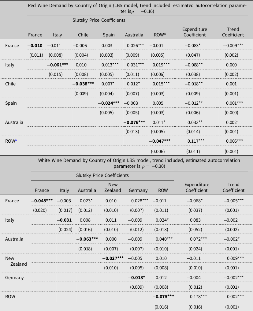
Table 2. Expenditure and Slutsky price elasticities of red and white wine demand by source country, LBS model, January 1990–October 2019

a All elasticities are “unconditional”, such that they are calculated based on total expenditures on all imported wine. Own price elasticities are denoted in bold characters.
b *, **, and *** indicate significance at the 10%, 5%, and 1% levels, respectively. Standard errors are in parentheses.
c ROW stands for Rest of the World.
The estimated demand elasticities for the broad groups of imported red, white, and other fresh grape wines are reported in Table 1. Footnote 3 The top panel of Table 1 has the expenditure and Slutsky (compensated) price elasticities, while the bottom panel reports the Cournot (uncompensated) price elasticities, conditional on total expenditures on imported wine. Expenditure elasticities for imported red, white, and other wines are all positive and statistically different from zero at the 1% significance level. Demand for imported red wine and imported white wine is expenditure inelastic, and demand for other imported fresh grape wines is expenditure elastic. In other words, the quantity demanded by US consumers of other fresh grape wines is more sensitive to a change in total expenditure for imported wines than that of imported red wine or imported white wine.Footnote 4 Marginal shares in Table 1 indicate how an additional dollar spent on imported wines would be allocated between red, white, and other imported grape wines. Accordingly, rounding differences aside, 42 cents of an additional dollar available for imported wine purchase would be spent on imports of other wines of fresh grapes, 36 cents would be spent on red wine, and 22 cents would be spent on white wine. On average, these marginal shares indicate a growing interest in other wine varieties over the sample period among US importers.
Slutsky and Cournot own-price elasticities for imported red wine, white wine, and other grape wine are all negative and statistically significant (Table 1). The Slutsky (compensated) own-price elasticity measures the percentage change in quantity demanded when own-price changes by 1%, keeping real total imported wine expenditure constant, and it measures the pure substitution effect of a price change on quantity demanded. Slutsky own-price elasticities for the three types of imported wine are all inelastic with the smallest in absolute value being for imported white wine (−0.11), followed by that of imported red wine (−0.16) and of other imported fresh grape wine (−0.57). The Cournot (uncompensated) own-price elasticities measure the percentage change in quantity demanded when own-price changes by 1%, keeping nominal total imported wine expenditure constant. Cournot price elasticities equal Slutsky price elasticities plus the (negative) income effect of a price change on quantity demanded. As such, Cournot own-price elasticities follow the same pattern as Slutsky own-price elasticities but are pairwise more negative (−0.33 for white wine, −0.52 for red wine, and −0.99 for other imported wine).
The Slutsky cross-price elasticities in Table 1 measure the percentage change in the quantity demanded of a product group i when the price of product group j increases by 1%, holding the real total expenditures on all imported wine constant. All six Slutsky cross-price elasticity pairs are significant. Imported red wine and imported white wine product groups are indicated to be complements, while the imported other wine group is a substitute for both the imported red and imported white wine groups. Four of the six Cournot cross-price elasticity pairs are statistically significant. Note that the Cournot cross-price elasticities are smaller than the corresponding Slutsky ones. In the case of imported white–imported other wines, the income effect of the cross-price change is larger in absolute value than the pure substitution effect, turning the positive Slutsky cross-price elasticities to become negative Cournot cross-price elasticities.
The demand elasticity estimates for red wine and white wine imports by exporting countries may be estimated in two ways. The first, conditional on total import expenditures for the particular wine type, are functions of the conditional demand equation parameters from equation (7); we henceforth call these conditional elasticities. Footnote 5 The second, conditional on total expenditure for all three imported wine groups (imported red, white, and other wines), are functions of parameters of both equations (7) and (6); henceforth, we refer to these elasticities as unconditional elasticities because they are determined by a broader measure of total expenditure than the conditional ones.Footnote 6 These unconditional demand elasticity estimates for red wine and white wine imports by exporting countries are reported in Tables 2 and 3, respectively. Table 2 provides expenditure and Slutsky (compensated) price elasticities for imported red wines by source in the top panel, and those for the imported white wine by source in the bottom panel, given total expenditures on all imported wine. Demand for imported red and white wines from all source countries is expenditure inelastic, and all Slutsky own-price elasticities for imported red wines are statistically significant and negative (Table 2). With an estimated own-price elasticity of −0.05, the quantity demanded of red wine from France responds the least to changes in its own price, holding real expenditures on imported wine constant. This finding is consistent with that reported by Seale, Marchant, and Basso (Reference Seale, Marchant and Basso2003).
Table 3. Cournot price elasticities of red and white wine demand by source country, LBS model, January 1990–October 2019

a All elasticities are “unconditional”, such that they are calculated based on total expenditures on all imported wine. Own price elasticities are denoted in bold characters.
b *,**, and*** indicate significance at the 10%, 5%, and 1% levels, respectively. Standard errors are in parentheses.
c ROW stands for Rest of the World.
The off-diagonal elements of the Slutsky price elasticity matrix in Table 2 (top panel) are the cross-price elasticities between pairs of imported red wines by countries of origin, and they indicate degrees of substitutability (or, complementarity) between red wine pairs imported from these countries. A positive Slutsky cross-price elasticity indicates that wines i and j are substitutes. As such, the quantity demanded of wine i increases when the price of wine j increases. A negative sign indicates that wines i and j are complements. Of the 30 Slutsky cross-price elasticities for imported red wines, 20 are statistically significant. A compensated percentage increase in prices of red wines from France, Italy, and Chile will increase the (compensated) quantity demanded of Australian red wine by 0.16%, 0.20%, and 0.09%, respectively; Australian red wine is a substitute for French, Italian, and Chilean red wines. Similarly, Spanish red wine is a substitute for Italian and Chilean red wines, and Chilean red wine is a substitute for Australian, Spanish, and ROW red wines. Italian red wine is a substitute for wines from Spain, Australia, and the ROW, but not for French wine. French wine is only substitutable with Australian red wine, and it complements red wine from Italy, Chile, and the ROW.
The bottom panel of Table 2 provides expenditure and Slutsky (compensated) price elasticities for imported white wines by source countries. Demand for imported white wine from all source countries (France, Italy, Chile, Spain, Australia, and ROW) is expenditure inelastic, given a percentage increase in total imported wine expenditures. All Slutsky own-price elasticities for imported white wines are negative and statistically significant at the 10% level or better. Conditional on (compensated) total expenditures on all imported wine, demand for imported white wines is price inelastic regardless of the country of origin. Italian white wine demand is the least price elastic, with an own-price elasticity of −0.12. Examining the off-diagonal elements of Slutsky price elasticity matrix in the bottom panel of Table 2 shows that fewer cross-price elasticities are statistically significant for white wine pairs than they are for red wine pairs. An interesting finding is that white wines from Italy and New Zealand cannot be substituted with any other imported white wine, holding (compensated) expenditures on total wine imports constant. A one percent increase in the (compensated) price of imported French white wine increases quantities demanded of German and Australian white wines by 0.37% and 0.17%, respectively. Conversely, a proportional increase in the price of Australian white wine leads to higher consumption of white wines from France and the ROW. French white wine is the only statistically significant substitute for German white wine.
Because Cournot cross-price elasticities are equal to the corresponding Slutsky elasticities plus a negative income effect of price changes, they do not indicate whether a good is a complement or a substitute. However, Cournot elasticities better reflect the overall market response to a price change than Slutsky cross-price elasticities. For instance, a Cournot cross-price elasticity may be negative, while the corresponding Slutsky cross-price elasticity is positive, if the income effect of a price change is larger in absolute value than the substitution effect of the same price change. The Cournot cross-price elasticities of imported red and white wine demand are presented in the top and bottom panels of Table 3, respectively. Cournot own-price elasticities for all red and white wines are statistically significant and continue to be less than one in absolute values. An interesting finding from a comparison between Cournot and Slutsky cross-price elasticities is that Australian red wine consumption becomes nonresponsive to price changes in French and Italian red wines after taking into account the income effects of these price changes (Table 3).
5. Simulated Welfare Effects of the October 2019 Tariffs
Simulations are used to evaluate the effects of the 25% US tariff increases imposed on red and white wines imported from some EU countries (i.e., France, Germany, Spain, and the United Kingdom) under the Section 301 enforcement of the US WTO rights in Large Civil Aircraft Dispute (84, Fed. Reg. October 9, 2019, 54245–54264). For both red and white wine imports, we only consider the scenario where the 25% tariff is fully passed onto the prices of tariff-imposed wines imported into the US. In particular, we assume that US domestic prices of French, Spanish, and German wines increase by 25% with the full pass-through of the 25% tariffs onto US importers. We also assume that US domestic prices of wines from non-taxed countries remain unchanged, implying a perfectly elastic supply curve for these countries. The assumption of a perfectly elastic import supply curve allows us to compute welfare implications while avoiding endogeneity. The simulation methods of Asci et al. (Reference Asci, Seale, Onel and VanSickle2016) and Zhang et al. (2020) are extended to measure tariff effects on quantities, expenditures by US importers (or, US consumers), receipts by exporting countries, and tariff revenues, as well as welfare measures of consumer surplus and deadweight loss. Note that producer surplus equals zero for all wines due to the assumption of horizontal (perfectly elastic) supply curves.
A tariff is a tax that places a wedge between the import demand curve and import supply curve, and the amount of the tariff that passes through to domestic consumers has implications for the prices received by exporters based on the elasticity of their import supply curve. The two extreme cases are when the import supply curve is vertical (perfectly inelastic) or horizontal (perfectly elastic). The more elastic is the import supply curve, the larger is the domestic price increase due to the tariff increase, and the smaller is the price reduction received by the suppliers of imported wines. In our simulation scenario, the full amount of the tariff is passed through to raise US prices of tariff-imposed European wines (i.e., French, Spanish, and German wines) by 25%. This is due to the perfectly elastic (horizontal) import supply curves for taxed EU wines resulting in no reductions in the prices received by suppliers of imported wines from the taxed EU countries. For imported wines not subject to the October 2019 tariffs, we assume 0% increases in their domestic prices, with perfectly elastic import supply curves. However, the demand curve for non-tariff wines may shift due to Cournot cross-price effects between wines sourced from taxed and non-taxed countries. As a result, the 25% tariff imposed on specific EU wines will have varying price and quantity effects on both taxed and non-taxed countries exporting wine to the US.
The baseline figures for quantities and expenditures are annual averages based on the last 12 months of data prior to imposing the additional tariff (i.e., November 2018–October 2019) and are reported in columns (3) and (4), respectively, for imported red and white wines in Table 4. Percent changes in quantities are calculated for each scenario by multiplying the appropriate Cournot elasticities from Table 3 times a 25% increase in imported French and Spanish red wine prices and a 25% increase in imported French and German white wine prices. Essentially, we calculate the effects of price changes of taxed wines on quantities demanded for both taxed and non-taxed wines for each of the six sources for imported red and the six sources for imported white wines. Based on the simulated quantity changes and a 25% (0%) increase in taxed (non-taxed) wine prices, we calculate the post-tariff expenditures and changes in expenditures on imported wines, post-tariff quantities of imported wines, tariffs collected, post-tariff receipts, and changes in receipts by source countries. The simulated cumulative effects of the US imposed 25% tariff increase on EU wines are reported in the top part of Table 4 for imported red wines and in the bottom part of Table 4 for imported white wines, with the effects being measured for one year forward.
Table 4. Simulated cumulative effects of 25% tariff on US imported European red and white wines

5.1. Cumulative Effects: Imported Red Wine
Based on a 25% increase in imported red wine prices from France and Spain and no price changes in other imported red wines in conjunction with a perfectly elastic supply curve for all supplying sources, total imported red wine quantity decreases by 3.7% or by 3.1 million gallons, with country-specific losses ranging from a 10.4% decrease in the imported quantity of Spanish red wine to a 0% change in the imported quantity for Australian red wine. Post-tariff total expenditure on imported red wine increases by 6.0% or by 124.2 million USD. Expenditures on French and Spanish red wines increase by 21.5% and 12.0%, respectively, while expenditures on non-taxed wines decrease for Italian red wine (2.1%), Chilean red wine (4.1%), and ROW red wine (6.2%), with no change in expenditure for Australian red wine. However, tariff revenues collected on French and Spanish red wines total 198.8 million USD; 164 million USD are collected on French red wine and 34.8 million USD on Spanish red wine. In addition, all suppliers of imported red wine lose revenue due to the differential tariff, except for Australian red wine. The total loss to suppliers of imported red wine to the US market is 74.6 million USD, ranging from a loss of 21.7 million USD for ROW red wine suppliers to a loss of 4.2 million USD for Chilean red wines.
5.2. Cumulative Effects: Imported White Wine
Based on a 25% increase in prices of imported white wine from France and Germany and no price changes for other country white wines in conjunction with a perfectly elastic supply curve for all supplying sources, total imported white wine quantity decreases by 1.3%, or by 1.1 million gallons, with country-specific losses ranging from a 5.9% decrease in the imported quantity of German white wine to a 0% change in the imported quantities of Italian and New Zealand white wines. Post-tariff total expenditure on imported white wine increases by 4.4% or by 75.0 million USD. Expenditures on French and German white wines increase by 21.1% and 27.7%, respectively, while expenditures on non-taxed wines decrease for Australian white wine (2.4%) and ROW white wine (5.9%), with no change in expenditures for Italian and New Zealand white wines. However, tariff revenues collected on French and German white wines total 96.8 million USD; 78.0 million USD are collected on French white wine and 18.8 million USD on German white wine. Unlike in the case of imported red wine suppliers, not all suppliers of imported white wine lose revenue after the tariff increase; suppliers of German white wine gain 1.6 million USD after the imposition of the differential tariff increases. In total, suppliers of imported white wine lose 21.8 million USD, with losses of 9.9 million USD endured by French white wine suppliers, 10.7 million USD by ROW white wine suppliers, and 2.8 million USD by Australian white wine suppliers.
5.3. Simulated Changes in Welfare
Welfare measures of consumer surplus and dead weight losses are calculated for the year following the US imposition of the 25% tariff increases on selected EU countries, utilizing the Cournot price elasticities from Table 3 that are calculated from the formulae presented in Appendix B, Table B1.Footnote 7 These welfare measures are reported in Table 5. Consumer surplus losses for imported red wines range from 4.2 million USD for imported Chilean red wine to 167.4 million USD for imported French red wine, with a total consumer surplus loss of 242.9 million USD; there is no consumer surplus loss for Australian red wine importers. Consumer surplus losses for imported white wines range from 10.7 million USD for ROW white wine to 79.2 million USD for French white wine, with a total consumer loss of 111.3 million USD; there are no consumer surplus losses associated with Italy and New Zealand white wines. In percentage terms, the changes for taxed wines are substantial with consumer surplus losses for French and Spanish red wines at 24.6% and 27.4%, respectively, and those for French and German white wines at 24.6% and 25.3%, respectively. As often is the case, dead weight losses as measured are small.
Table 5. Simulated welfare effects of 25% tariffs on US imported European red and white wines

6. Conclusions
This paper develops a consumer demand framework to estimate changes in import demand due to 25% tariff increases imposed on select EU wine exporters in October 2019 and to measure the welfare effects of these changes by source country. Simulated welfare measures capture tariff effects on both taxed and non-taxed countries due to non-zero cross-price effects for taxed and non-taxed wine imports.
Simulated revenue and welfare effects of the tariff on select EU countries reflect the highly differentiated nature of the discriminatory tariff increases. For the taxed wines from the selected EU countries, post-tariff changes in revenue are negative for suppliers of French and Spanish red wines and for suppliers of French white wines, but are positive for German white wine suppliers. In addition, revenue losses associated with ROW red and white wines are larger than those of the taxed wines. These results are, in part, due to prices of taxed wines affecting quantities demanded of non-taxed wines through non-zero Cournot cross-price elasticities. It is also due to the simulation assumption of the infinitely elastic supply curve for imported wines. As such, the calculated revenue losses are likely to be a lower end estimate of the effect on post-tariff revenues. Simulations that take into account inelastic supply curves that would allow prices of non-taxed wines to increase in response to price increases of taxed wines may find larger revenue losses for both taxed and non-taxed wine suppliers.
What is clear is that the full pass-through of the 25% tariff increases to prices of taxed wine imports in the domestic market harms US consumers, with consumer losses for the taxed wines at about 25% compared to the consumer surplus prior to the imposition of the discriminatory tariff. While consumer surplus losses are smaller for the non-taxed wines, they are still harmful to US consumers of imported wines.
While the research is an ambitious first attempt to merge consumer (import) demand theory with tariff theory, it is successful in several ways. On the consumer theory side, expenditure and price elasticities that measure the joint effects of price and expenditure changes from group demand and from demand for wine type by source country are derived and used successfully to measure changes in revenue received by suppliers of imported wine into the US market as well as consumer surplus and dead weight losses. Because the simulations are based on a system of import demand equations, it allows for the measurement of revenue and welfare effects from cross-price changes that can shift import demand curves. As far as the authors are aware, this is the first paper to do so. Finally, the paper applies these innovations to an interesting case of a discriminatory tariff and examines how these tariffs affect taxed and non-taxed imports differently.
Acknowledgments
The authors are grateful for the useful comments and suggestions made by the editor and the two anonymous reviewers. Seniority of authorship is not assigned.
Author Contributions
Conceptualization, G.O., J.L.S, Jr., and L.Z; Methodology, J.L.S, Jr., L.Z., and G.O.; Formal Analysis, J.L.S, Jr. G.O., and L.Z. Data Curation, L.Z., and J.L.S, Jr.; Writing—Original Draft, L.Z. Writing—Review and Editing, G.O., and J.L.S, Jr.
Conflict of Interest
Lisha Zhang, Gulcan Onel, and James L. Seale, Jr. declare none.
Data Availability Statement
The data that support the findings of this study are openly available in Global Agricultural Trade System at https://apps.fas.usda.gov/gats/default.aspx and in Current Population Survey at https://www.census.gov/cps/data/cpstablecreator.html
Funding Statement
This research received no specific grant from any funding agency, commercial or not-for-profit sectors.
Appendix A. Additional Results
Table A1. Descriptive statistics on US consumption of imported red and white wine by source country, January 1990–October 2019

Table A2. Functional form selection

Table A3. Homogeneity, symmetry, and model specification tests

Table A4. Estimated parameters of the demand system for three wine groups, differential AIDS, January 1990–October 2019

Table A5. Estimated parameters of red and white wine demand by country of origin
Appendix B. Computation of Elasticities
Table B1. Marginal share, Slutsky price term, and elasticity formulas for the selected functional forms
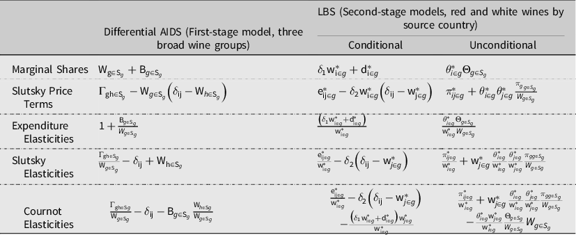
Notes: Where  ${\rm{\theta }}_{i \in g}^* = \left( {{{\rm{\delta }}_1}{\rm{w}}_{i \in g}^* + {\rm{d}}_{i \in g}^*} \right)$
,
${\rm{\theta }}_{i \in g}^* = \left( {{{\rm{\delta }}_1}{\rm{w}}_{i \in g}^* + {\rm{d}}_{i \in g}^*} \right)$
,  ${\Theta _{g \in {S_g}}} = \left( {{\delta _1}{{\rm{W}}_{g \in {S_g}}} + {{\rm B}_{g \in {S_g}}}} \right)$
, and
${\Theta _{g \in {S_g}}} = \left( {{\delta _1}{{\rm{W}}_{g \in {S_g}}} + {{\rm B}_{g \in {S_g}}}} \right)$
, and  ${\rm{\pi }}_{{\rm{ij}} \in g}^*{\rm{ = e}}_{{\rm{ij}} \in g}^* - {\delta _2}{\rm{w}}_{i \in g}^*\left( {{{\rm{\delta }}_{{\rm{ij}}}} - {\rm{w}}_{{\rm{j}} \in g}^*} \right)$
in the last column. Unconditional elasticities are computed in relation to first-stage values and total imported wine expenditures.
${\rm{\pi }}_{{\rm{ij}} \in g}^*{\rm{ = e}}_{{\rm{ij}} \in g}^* - {\delta _2}{\rm{w}}_{i \in g}^*\left( {{{\rm{\delta }}_{{\rm{ij}}}} - {\rm{w}}_{{\rm{j}} \in g}^*} \right)$
in the last column. Unconditional elasticities are computed in relation to first-stage values and total imported wine expenditures.


 Open access