


1. Introduction
We assess the economic impact of various negative and positive shocks on outcomes and welfare for the heterogeneous agents along the vertical tree fruit supply chain, from the producer to a wholesale intermediary and then to the consumer. Gotsch and Wohlegnant (Reference Gotsch and Wohlgenant2001) show the importance of a segmented supply chain in modeling commodity markets. Our contribution is to model the tree fruit packing and processing intermediaries—something that has not been done in the literature—to better assess the full economic outcomes and welfare impacts from either a negative or a positive shock.
To measure economic consequences of a shock on each of the agents in the supply chain, we develop an intertemporal equilibrium displacement model of demand and supply with international trade (Harrington and Dubman, Reference Harrington and Dubman2008). We draw on similarities in the modeling of perennial tree fruit and livestock (Paarlberg et al., Reference Paarlberg, Seitzinger, Lee and Mathews2008; Pendell et al., Reference Pendell, Brester, Schroeder, Dhuyvetter and Tonsor2010) in developing our equilibrium displacement model. Our modeling innovation is to expand the tree fruit supply chain from producers and consumers to be more complete. The addition of two intermediaries—one for the fresh market and one for the processed market—allows our model to better capture how a shock affects the separate parts of the supply chain. Because the long life cycle of perennial trees tends to make suppliers less responsive to sudden market shocks and prices in the short term (Zhao, Wahl, and Marsh, Reference Zhao, Wahl and Marsh2007), our equilibrium displacement model is intertemporal. The model is general and could be applied to other tree fruit, countries, or size and type of single or multiple exogenous shocks. As an illustration, we apply the parameters for the U.S. pear fresh and processed markets to the model and simulate outcomes from various kinds and sizes of shock. From the simulated outcomes, we calculate welfare effects for growers, packers and processors, and consumers. Though we illustrate our model with the tree fruit industry, it could be used for other perennial commodities that feature multiple output goods with intermediaries, such as the application to grapes in Ahn and Im (Reference Ahn and Im2016).
We consider the effects to the intermediaries from three different kinds of shock. The first is a negative supply shock that should be thought of as a pest or disease outbreak. The second shock we consider is a tightening of the regulations imposed by a foreign government for exporting into that market. The Sanitary and Phytosanitary Measures (SPS) Agreement and the Technical Barriers to Trade Agreement allow countries to set regulatory standards. The third shock is a positive shock to foreign demand, in conjunction with an increase in the trade cost in order to show how our model can handle multiple simultaneous, and opposing, shocks.
Estimating the economic consequences of negative and positive shocks has a long history. Similar to our study in spirit if not in method, Paarlberg, Lee, and Seitzinger (Reference Paarlberg, Lee and Seitzinger2003) argue that welfare impacts from an outbreak of foot-and-mouth disease must be decomposed into subgroups of producers and consumers to be accurately measured. On trade cost shocks, Calvin, Krissoff, and Foster (Reference Calvin, Krissoff and Foster2008) estimate that phytosanitary requirements on U.S. fresh apple imports into Japan increase the trade cost by 15¢ per pound and an additional 5¢ per pound in accounting cost. Peterson and Orden (Reference Peterson and Orden2008) show U.S. net welfare increased by $77 million because of a decrease in a seasonal trade barrier with Mexico on the importation of fresh Hass avocados in 2004. Peterson et al. (Reference Peterson, Grant, Roberts and Karov2013) find statistically and economically significant negative trade impacts from SPS regulations initially (though they also find the effect of restrictive measures can be overcome with time and learning).
All of these studies, as well as many others, only consider the impacts to growers and consumers. None emphasize the effects on packers and processors for the tree fruit sector. A better understanding of the distribution of benefits and costs from a shock assists the industry, and possibly the government, in efficiently guiding resource allocations.
2. A Tree Fruit Market Model with Intermediaries
We develop an intertemporal economic model of a single tree fruit crop. We model domestic fresh and processed tree fruit demand, supply, and international trade from growers to packers and processors and up to consumers. The model allows for the assessment of an exogenous negative or positive shock, such as, but not limited to, a disease or pest outbreak, trade sanctions, and increased foreign demand of varying levels. We calculate the change to prices, production, value added, trade, and welfare for each segment of the supply chain, though for brevity we restrict our reported analysis to grower prices and welfare. We consider two types of products: fresh and processed produce. Details of the pear industry may be found in Appendix A.
On the supply side, a dynamic supply response model is necessary to capture the nature of tree fruit. After planting, a fruit tree takes several years to mature, and then it is commercially productive for several decades. Total supply per period, which because of the time for tree maturity is fixed in the short run, is bearing acreage multiplied by yield per acre. On the demand side, aggregating by population over a per capita demand equation provides parameters used to estimate gross and net benefits to the industry from an exogenous shock. On the international side, imports and exports are linked through market-clearing price conditions at the level of the intermediaries. The model includes a trade policy instrument that can be modified by the degree of government regulatory response, reg.
Each season, fruit produce passes through three levels of the supply chain: the farm (producer) level, a wholesale (intermediary) level, and a retail (consumer) level. This may be seen in Figure 1. The intermediary for fresh produce is a packer. The intermediary for processed produce is a processor. Fresh and processed fruit allocation is determined by prices, given that total production is fixed in the short run. Then, for each year, for each product type, fruit is allocated to the domestic and international markets through a market-clearing condition at the wholesale level so that domestic supply plus imports equals domestic consumption plus exports. Farm-level and retail-level prices are identified through marketing margins based on the wholesale price benchmark. The mathematical details of the model may be found in Appendix B.
Figure 1. A Model of Fresh and Processed Tree Fruit Markets with Intermediaries
We exogenously shock the model. The effect is realized as a change in the model's retail-level equilibrium prices and induces upstream dynamic supply responses. The estimated dynamic supply response, along with the wholesale-level market-clearing conditions each year, allows us to compare the simulation results from the shock to the baseline economy over time.
2.1. Farm-Level Supply and Demand
The production of perennial fruit involves planting, yield, and removal. It has been known since at least French and Matthews (Reference French and Matthews1971) that the age distribution of plantings of perennials is important in estimating the effects of a shock. Growers plant new trees and remove existing acreage to maximize profits over time. The acreage equation for fruit trees next period is given by K
j + 1
t + 1 = Kt
j
− RMj
t
, Kt
0 = NPt
, where Kj
t
is the acres of age j trees at year t, RMj
t
is the acres removed of age j trees in year t, and NPt
is the acres of new plantings in year t. Assuming pear trees start to bear fruit at age 3 and stop at age μ if not removed, ${B_t} = \mathop \sum _{j = 3}^\mu K_t^j$
is the bearing acreage in period t. The change in bearing acreage from this period to the next period absent an exogenous shock is
${B_t} = \mathop \sum _{j = 3}^\mu K_t^j$
is the bearing acreage in period t. The change in bearing acreage from this period to the next period absent an exogenous shock is $\Delta {B_t} = {B_{t + 1}} - {B_t} = N{P_{t - 2}} + \mathop \sum _{j = 3}^\mu RM_t^{j}$
.
$\Delta {B_t} = {B_{t + 1}} - {B_t} = N{P_{t - 2}} + \mathop \sum _{j = 3}^\mu RM_t^{j}$
.
Yield per acre depends on technology, such as rootstock structure. To capture these characteristics, we assume the yield in n years is y t + n = (1 + g) n yt , which is the yield in the current year yt scaled by a growth rate g. Figure 2 shows evidence of this growth rate in yield per acre, along with a 3-year moving average of the data.
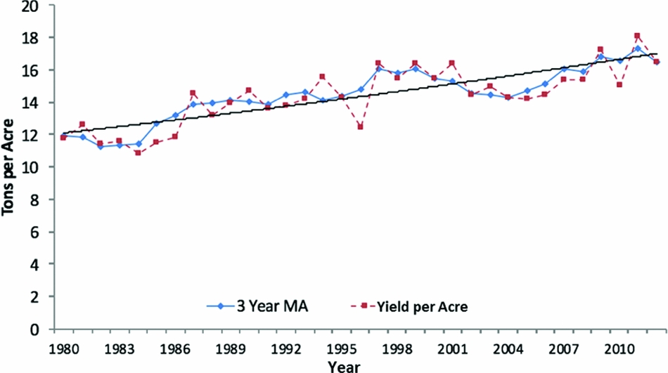
Figure 2. Yield: 3-Year Yield Moving Average (MA) and Constant Technological Change (source: U.S. Department of Agriculture, National Agricultural Statistics Service, 2016)
The next period farm-level supply, FS t + 1, is obtained by multiplying the yield and bearing acreage:
 $$\begin{equation}
F{S_{t + 1}} = {S_{t + 1}}{y_{t + 1}}{B_{t + 1}} = {S_{t + 1}}\left( {1 + g} \right){y_t}\left( {\Delta {B_t} + {B_t}} \right),
\end{equation}$$
$$\begin{equation}
F{S_{t + 1}} = {S_{t + 1}}{y_{t + 1}}{B_{t + 1}} = {S_{t + 1}}\left( {1 + g} \right){y_t}\left( {\Delta {B_t} + {B_t}} \right),
\end{equation}$$
where S t + 1 is the size of an exogenous shock on supply. Thus, in principle, we can calculate the next period's supply from this period's data and the shock.
In our counterfactual scenarios, we have to predict the change in bearing acreage, ΔBt , from the equilibrium values from the previous periods. To do that, we use a modified French and Matthews (Reference French and Matthews1971) reduced-form econometric model to estimate the bearing acreage in the next period:
 $$\begin{equation}
\Delta {B_t} = {\beta _0} + {\beta _1}\Delta {B_{t - 1}} + {\beta _2}\Delta {p^e} + {\beta _3}\overline {{B_{t - 2}}} + {\beta _4}\overline {{Y_{t - 2}}} + {\beta _5}t + {\mu _t}.\
\end{equation}$$
$$\begin{equation}
\Delta {B_t} = {\beta _0} + {\beta _1}\Delta {B_{t - 1}} + {\beta _2}\Delta {p^e} + {\beta _3}\overline {{B_{t - 2}}} + {\beta _4}\overline {{Y_{t - 2}}} + {\beta _5}t + {\mu _t}.\
\end{equation}$$
In equation (2), the change in bearing acreage is recursive as seen by the inclusion of the Δβ
t − 1 term. The recursive bearing acreage term captures the dynamics from plantings that occurred two periods ago and will not mature until next period. We also include the change in the previous period's j-year moving average of real producer price, $\ {\rm{\Delta }}{p^e} = \frac{1}{j}( {\sum\nolimits_{h = 0}^{j - 1} {{p_{t - 1}}} - \sum\nolimits_{h = 0}^{j - 1} {{p_{t - 1 - h}}} } )$
; the k-year moving average of bearing acreage ending at t − 2,
$\ {\rm{\Delta }}{p^e} = \frac{1}{j}( {\sum\nolimits_{h = 0}^{j - 1} {{p_{t - 1}}} - \sum\nolimits_{h = 0}^{j - 1} {{p_{t - 1 - h}}} } )$
; the k-year moving average of bearing acreage ending at t − 2, $\overline {{B_{t - 2}}} = \frac{1}{k}\sum\nolimits_{h = 0}^{k - 1} {{B_{t - 2 - h}}} $
; the m-year moving average of yield per acre ending at t − 2,
$\overline {{B_{t - 2}}} = \frac{1}{k}\sum\nolimits_{h = 0}^{k - 1} {{B_{t - 2 - h}}} $
; the m-year moving average of yield per acre ending at t − 2, $\overline {{Y_{t - 2}}} = \frac{1}{m}\sum\nolimits_{h = 0}^{m - 1} {{y_{t - 2 - h}}} $
; a time trend, t; and an error term, μ
t
. The lag lengths j, k, and m are determined empirically in the econometric modeling. All of the variables can be calculated from the real-world or simulated data, which is why we use price instead of profit as in French and Matthews (Reference French and Matthews1971). A change in the moving average of real producer pear price, Δpe
, is important as it is the expectation of the future equilibrium price. Our use of moving averages replaces fixed behavior from a previous period with a dynamic process to capture growers’ expectations evolving over time.
$\overline {{Y_{t - 2}}} = \frac{1}{m}\sum\nolimits_{h = 0}^{m - 1} {{y_{t - 2 - h}}} $
; a time trend, t; and an error term, μ
t
. The lag lengths j, k, and m are determined empirically in the econometric modeling. All of the variables can be calculated from the real-world or simulated data, which is why we use price instead of profit as in French and Matthews (Reference French and Matthews1971). A change in the moving average of real producer pear price, Δpe
, is important as it is the expectation of the future equilibrium price. Our use of moving averages replaces fixed behavior from a previous period with a dynamic process to capture growers’ expectations evolving over time.
Equation (2) may be used to predict the change in bearing acreage from the shock in period t onward. In Section 3, we show the estimated coefficients and how equation (2) performs compared with the data. These equations capture that a shock to yield is short term because fruit trees are perennial, but a shock to bearing acres is long term because of the time for new plantings to mature.
Whether production enters the fresh or processed market is determined by farm-level prices.Footnote 1 Farm-level demand for fresh pears is FDf,t = FPf (pF f,t, FSt ). We impose a market-clearing condition each year so that the allocation of fruit to the processed market is the total production minus the quantity distributed to the fresh market: FDp,t = FSt − FDf,t . This ensures the equality of farm-level demand with supply in equilibrium.
In our model, the market for selling fruit at the producer level is competitive so that producer price equals producer marginal cost in equilibrium. Wann and Sexton (Reference Wann and Sexton1992) provide support that producer price in the U.S. pear market is not significantly different from marginal cost.
2.2. Retail-Level Demand and Supply
We sum individual demand for pears to that of the population in order to account for domestic population growth. For individual demand, q is a vector of the two commodities available, p is a vector of corresponding prices, and income is I. We define z to be other conditioning or shift variables (period t subscripts are omitted). Then the consumer's maximization problem is $\mathop {\max }_q \{ {u(q;z)|p^{\prime}q \le I} \}$
, where u(q; z) reflects the individual's utility function with standard properties (Deaton and Muellbauer, Reference Deaton and Muellbauer1990). Solving this yields the individual consumer's demand:
$\mathop {\max }_q \{ {u(q;z)|p^{\prime}q \le I} \}$
, where u(q; z) reflects the individual's utility function with standard properties (Deaton and Muellbauer, Reference Deaton and Muellbauer1990). Solving this yields the individual consumer's demand:
 $$\begin{equation}
q_i^D = f_i^D(p_f^R,p_p^R,I,z),
\end{equation}$$
$$\begin{equation}
q_i^D = f_i^D(p_f^R,p_p^R,I,z),
\end{equation}$$
where qD i is the consumption of retail product i, and pR f and pR p are retail prices for fresh and processed fruit, respectively. With a homothetic utility function, the individual demand function (equation 3) can be linearly summed to construct aggregate quantity demanded for each price. We assume the domestic population will grow constantly. We find national retail-level demand by multiplying the individual retail-level demand by the number of consumers as given by the population (pop) of the U.S. domestic market:
 $$\begin{equation}
Q{D_i} = pop \cdot q_i^D.
\end{equation}$$
$$\begin{equation}
Q{D_i} = pop \cdot q_i^D.
\end{equation}$$
2.3. International Trade
We model the exports and imports of fresh and processed fruit at the wholesale level of the packers and processors. Trade is determined by the U.S. domestic price along with an additional trade cost.Footnote 2 That cost represents the added expense of shipping and international transactions.
The parameter γ ei , ranging from 0 to 1, indicates the severity of trade restrictions and regulations imposed by foreign governments. Zero is the most severe and represents a complete blockade. Let Ei be the quantity demanded by the international market:
 $$\begin{equation}
{E_i} = f_i^{Ex}(p_i^W - c_i^{SPS}) \cdot {\gamma _{{e_i}}},
\end{equation}$$
$$\begin{equation}
{E_i} = f_i^{Ex}(p_i^W - c_i^{SPS}) \cdot {\gamma _{{e_i}}},
\end{equation}$$
where fEx i ( · ) is the excess supply function for product type i, pW i is wholesale price for product type i, and cSPS i is the cost imposed by the SPS conditions.
Import demand in the United States for foreign fruit products is also a function of the domestic price and trade costs. We assume that foreign and domestically produced fruit are substitutes. Let Mi be the quantity of the imported fruit:
 $$\begin{equation}
{M_i} = f_i^{{\mathop{\rm Im}\nolimits} }(p_i^W - {t_{{m_i}}}),
\end{equation}$$
$$\begin{equation}
{M_i} = f_i^{{\mathop{\rm Im}\nolimits} }(p_i^W - {t_{{m_i}}}),
\end{equation}$$
where $f_i^{{\mathop{\rm Im}\nolimits} }( \cdot )$
is the excess demand function for product type i, and t
mi
is the trade cost. Combining equations (5) and (6) yields domestic retail-level supply:
$f_i^{{\mathop{\rm Im}\nolimits} }( \cdot )$
is the excess demand function for product type i, and t
mi
is the trade cost. Combining equations (5) and (6) yields domestic retail-level supply:
 $$\begin{equation}
Q{S_i} = F{S_i} + {M_i} - {E_i}.
\end{equation}$$
$$\begin{equation}
Q{S_i} = F{S_i} + {M_i} - {E_i}.
\end{equation}$$
Thus, with market-clearing prices, retail-level supply is the total production of each product type plus imports minus exports of each product type.
2.4. Wholesale-Level Intermediaries and Market Closure
The packers and processors at the wholesale level have an important role in connecting farm and retail-level markets. Yet this is a group that is often not explicitly modeled in studies of tree fruit or other commodities. We introduce this group into our model by making it the center point for market-clearing prices. That is, our model is designed so that a normalized baseline wholesale price clears the wholesale market for fresh and processed fruit each year. Then we apply price margins on the wholesale price to get the farm and retail prices.
The relationship between grower-received price and wholesale price is pF i = pi W − MMF i , where pF i is the growers’ price for product type I, and MMF i is the markup price between the farm level and the wholesale level. The relationship between retail-received price and wholesale-received price is given by pR i = pi W + MMR i , where pR i is the retail-level price for product type i, and MMR i is the markup between intermediaries to consumers.
Because the wholesale market clears, equation (4) equals equation (7) and may be written as follows:
 $$\begin{equation}
Q{D_i} + {E_i} = F{S_i} + {M_i},
\end{equation}$$
$$\begin{equation}
Q{D_i} + {E_i} = F{S_i} + {M_i},
\end{equation}$$
where QDi is the quantity demand of i at domestic retail market. Using the markup price equations, the partial equilibrium wholesale price is solved from the marketing-clearing conditions.
3. Data and Performance of Bearing Acres Predictor
The model is parameterized using data from the U.S. pear industry. The Noncitrus Fruits and Nuts Summaries (U.S. Department of Agriculture [USDA], National Agricultural Statistics Service, 2016) provides data on U.S. pear acreage, yield, and grower prices. These are the data we need to estimate the coefficients in equation (2). For the rest of the model, trade volume and prices for fresh and processed pears are from the Foreign Agricultural Service's (FAS) Global Agricultural Trade System (USDA-FAS, 2016). Per capita consumption of fruit is from the Food Availability Data System (USDA, Economic Research Service, 2016). Wholesale price for fresh pears is from the USDA Agricultural Marketing Service (2017), and retail price for fresh pears is from the U.S. Department of Labor, Bureau of Labor Statistics. A detailed description of the U.S. pear industry may be found in Appendix A. We take the population of the United States from the U.S. Department of Commerce, Bureau of the Census (2016). We deflate prices into 2010 dollars and use a 4% discount rate to calculate net present value. See Table 1 for the values we use as parameters and their sources.
Table 1. Parameter Description and Values
Sources: aPrice and Mittelhammer (Reference Price and Mittelhammer1979), bAndersen and Sexton (Reference Andersen and Sexton2001), cassumed values, and destimated values.
From the data listed previously, we estimate the coefficients in equation (2):
 $$\begin{equation*}
\Delta {\overset{\scriptscriptstyle\frown}{B}_t} =
\mathop {{{\hbox{14,937.00}}^{***}}}\limits_{({2,429.63})}+
\mathop {{{0.32}^{***}}}\limits_{(0.09)}\Delta {B_{t - 1}} +
\mathop {{{6.39}^{**}}}\limits_{(3.13)} \Delta {p^e} -
\mathop {{{0.16}^{***}}}\limits_{(0.03)} {\overline{{B}_{t - 2}}} -
\mathop {{{234.32}^{**}}}\limits_{(117.09)}{\overline{{Y}_{t - 2}}} -
\mathop {{{28.59}^*}}\limits_{(16.70)} t,
\end{equation*}$$}
$$\begin{equation*}
\Delta {\overset{\scriptscriptstyle\frown}{B}_t} =
\mathop {{{\hbox{14,937.00}}^{***}}}\limits_{({2,429.63})}+
\mathop {{{0.32}^{***}}}\limits_{(0.09)}\Delta {B_{t - 1}} +
\mathop {{{6.39}^{**}}}\limits_{(3.13)} \Delta {p^e} -
\mathop {{{0.16}^{***}}}\limits_{(0.03)} {\overline{{B}_{t - 2}}} -
\mathop {{{234.32}^{**}}}\limits_{(117.09)}{\overline{{Y}_{t - 2}}} -
\mathop {{{28.59}^*}}\limits_{(16.70)} t,
\end{equation*}$$}
where N = 75, $\widehat{R^2} = 0.72$
, and asterisks (***, **, and *) indicate significance with 99%, 95%, and 90% confidence, respectively. We choose the variables to include and the lengths of the moving averages based on goodness-of-fit statistics. We use a 3-year moving average for price, 5 years for bearing acreage, and 5 years for yield.
$\widehat{R^2} = 0.72$
, and asterisks (***, **, and *) indicate significance with 99%, 95%, and 90% confidence, respectively. We choose the variables to include and the lengths of the moving averages based on goodness-of-fit statistics. We use a 3-year moving average for price, 5 years for bearing acreage, and 5 years for yield.
The change in 3-year moving average of price plays a large role in the decision to expand bearing acreage as economic intuition suggests. If growers expect the price of pears to increase, they want more sales through greater output, per the law of supply, and can achieve that through additional plantings and delayed removals. On the other hand, the 5-year average bearing acreage and 5-year average yield per acre have a statistically significant negative effect on the change in bearing acreage as expected. An increase in yield per acre either reduces growers’ incentive to expand orchards or accelerates the incentive to remove old trees and replant. Average bearing acreage during the previous 5 years at year t − 2, ${\overline{{B}_{t - 2}}}$
, is a good indicator for old trees that must be removed in the next few years. If the proportion of old trees is higher, then the change in bearing acreage would decrease from removals. Note the effect of the moving average of previous yields cannot be directly compared to the much smaller coefficient on moving average of previous bearing acreage because of the different units. The time trend is negative as expected.
${\overline{{B}_{t - 2}}}$
, is a good indicator for old trees that must be removed in the next few years. If the proportion of old trees is higher, then the change in bearing acreage would decrease from removals. Note the effect of the moving average of previous yields cannot be directly compared to the much smaller coefficient on moving average of previous bearing acreage because of the different units. The time trend is negative as expected.
The effect of the change in bearing acres from the previous period, Δβ t − 1, is positive for the change in bearing acreage and statistically significant. It has the opposite sign as the moving average on the number of bearing acres from three to seven periods ago. The positive coefficient on the lagged change in bearing acreage term is accounting for short-run dynamics and the cyclicality of bearing acres that is not captured by the moving average terms. By including the lagged change in bearing acreage term, the Durban-Watson statistic is 2.062, suggesting no autocorrelation.
To assess the quality of our predictor, we compare its performance to the data. As can be seen in Figure 3, our estimates largely match the historical data albeit with less volatility. That is because our estimator uses moving averages and thus must be less volatile than the data. One may also see in Figure 3 that the change in bearing acres is cyclical in the sense that it does not change from positive to negative year to year, but rather stays positive or negative for a few years before switching.
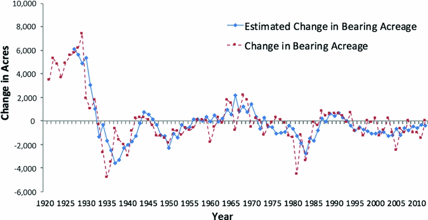
Figure 3. Change in Bearing Acreage versus Estimated Change in Bearing Acreage
4. Scenarios
We consider three exogenous shocks to the model. These are (1) a negative supply shock in bearing acreage representing a pest or disease outbreak, (2) an increase in export costs representing an increase in the SPS barriers imposed by all of the foreign governments of the world, and (3) a combination of an SPS barrier increase along with a positive export shock. Each shock, which we discuss in turn, occurs in 1 year only. We consider three levels of magnitude compared to the baseline for each shock: low, medium, and high.Footnote 3 That gives one baseline no-shock scenario and nine comparison scenarios. The model begins in 2002 and runs through two life cycles of pear trees, which is 60 years. The shock occurs in 1 year, 2015, so there are 13 years for the model to match the data before the shock occurs.
-
• Scenarios A: A reduction in bearing acreage of 4%, 8%, and 12%.
-
• Scenarios B: A tightening of regulations imposed by the foreign government on U.S. exports that results in a trade contraction of 3%, 6%, and 9% for fresh and processed pears.
-
• Scenarios C: A 3% tightening of SPS regulations and an increase in foreign demand resulting in a trade expansion of 3%, 6%, and 9% for fresh and processed pears.
The empirical model was calibrated as an equilibrium displacement model using the parameters in Table 1 (Jiang, Reference Jiang2013). In order to ensure the results are robust to selected parameter values, in particular those for the price elasticity of fresh and processed pears, we follow the Bayesian approach to sensitivity analysis advocated by Davis and Espinoza (Reference Davis and Espinoza1998) and applied by Richard and Sumner (Reference Rickard and Sumner2008). We report expected estimates from 500 Monte Carlo simulations. For the reported results, we show the value from the parameters listed in Table 1 along with the values of the 90% confidence intervals obtained by ordering the results of these 500 repetitions.
5. Results, Welfare, and Net Present Value
A shock directly or indirectly changes the number of bearing acres compared to the baseline. That translates directly into changes in the grower price. We calculate the baseline grower price path and price changes from each shock and describe the outcomes in each scenario in terms of grower price. We could also describe the outcomes in terms of production, value added, or other variables. For the sake of brevity, we focus our analysis on grower prices and welfare. The grower price is calculated as an average price of farm-level fresh and processed pear prices weighted by utilization production. Of course, the larger the magnitude of the shock, the more pronounced the impact.
5.1. Negative Supply Shock, Scenarios A
In the negative supply shock on bearing acreage in scenarios A, the grower price is higher than baseline right after the outbreak. This is because the reduced supply of pears stemming from the loss of bearing acres drives up the price. An upward trend that follows the initial price increase is driven by the domestic population growth. As the grower price increases, foreign pears become relatively more attractive to domestic consumers, and domestic pears become less attractive to foreign buyers. Thus, there is a net-trade effect. The influx of foreign pears causes downward pressure on the grower price. Lower price causes growers to reduce their plantings, which in turn causes upward pressure on the domestic price. The lag in time for plantings to mature means the domestic price from the shock overshoots the benchmark price, causing growers to increase plantings, and the cycle repeats. All the while, the effects of net trade act to dampen the domestic price effects. Therefore, the grower price exhibits a diminishing, oscillating pattern regulated by fluctuations in net trade that slowly converges to the long-run equilibrium. Overall, there is a decrease in domestic consumption overall for both processed and fresh pears.
Domestic consumer benefits associated with a negative supply shock are calculated as change in consumer surplus relative to the baseline reflecting the effects of both price changes and quantities demanded. (See Appendix B for the calculation details.) Figure 4a shows the time path of changes in consumer surplus for fresh pears. The pattern for processed pears is essentially identical qualitatively, though larger in magnitude quantitatively, and is omitted. Consumers are worse off when the retail price fluctuates above the baseline as a result of the supply shock. Consumers, however, benefit when the quantity of bearing acres recovers following the shock and price drops below the baseline. The magnitude of the change in consumer surplus is because of the large population of the United States.
Figure 4. Negative Supply Shock (scenario A) Consumer, Producer, and Intermediary Surplus (fresh) Relative to Baseline, 2002–2062
Producer surplus is calculated as the change in the share of total revenue that accrues to capital and management from the shock compared to the benchmark. The rates are given in Table 1. (See Appendix B for the calculation details.) The experience of producers is the opposite of consumers because when prices are low, producers are harmed. This is seen in Figure 4b. The initial supply shock increases prices in the short run and benefits producers. However, the loss of crop and the subsequent replanting causes prices to drop in the medium run. Producers, however, can be worse off even if prices are above the baseline because of the need and cost to replant, which drives down revenues. Because of the lag between the investment decision and the realization of that decision, the effect on bearing acreages is not observed until the trees reach reproductive maturity. The increase in bearing acres results in increased production driving down prices and revenue and dissipating the benefits for producers.
The surplus change to the intermediary follows the qualitative pattern of the producer but is quantitatively larger. This is seen in Figure 4c. That the intermediary change in surplus is about twice that of the producer shows the importance of modeling the intermediary as without it those surplus changes would be attributed to growers. A traditional producer-consumer model would misstate the distribution of shock effects to industry agents. Furthermore, the greater the severity of the shock, the larger the quantitative impact to the intermediary relative to the producer.
5.2. Negative Trade Cost Shock, Scenarios B
Unlike the pattern in scenarios A, grower prices in scenarios B are initially less than those of the baseline. This is because the declines in exports are rerouted to domestic supply and drive down the equilibrium price. However, the impacts of the trade shock are relatively short lived on production compared with the shock to bearing acres, though grower prices in scenarios B never quite reach those of the baseline. The increasing trend from population growth mitigates some of the decrease in price. The harm from a tightening of trade regulations is less impactful than a direct shock to the number of bearing acres because the supply is the same in the case of a trade shock. It is just the distribution of consumption that changes, whereas the quantity supplied changes in a shock to bearing acres.
Domestic consumers benefit from a negative trade cost shock as that diverts more quantity supplied into the domestic market and lowers retail price. Figure 5a shows the change in consumer surplus for fresh pears. As can be seen from the y-axis, the effect of the trade shock in terms of consumer surplus is much less than from the supply shock. Producers lose surplus from the increased trade cost because of the decrease in price. The initial price decrease is short lived compared with the supply shock, but it still takes 20 or more years for prices to approach baseline. Unlike in scenarios A, the initial surplus change of the intermediary is about 75% of the producer surplus change. Therefore, our model shows that the type of industry shock affects the distribution of the effects between producer and intermediary.
Figure 5. Negative Trade Cost Shock (scenario B) Consumer, Producer, and Intermediary Surplus (fresh) Relative to Baseline, 2002–2062
5.3. Positive Foreign Demand Shock and SPS Increase, Scenarios C
To demonstrate the impacts of multiple simultaneous shocks, scenarios C are a 3% increase in the SPS barriers and also an increase in exports from greater foreign demand. The increase in the trade cost is realized as an immediate reduction in net trade for fresh and processed fruit and thus an immediate reduction in grower price. The effect of that negative shock to the trade cost is short lived though, as the positive foreign demand shock kicks in to increase the retail and grower price.
With more total demand, the grower price is larger than in the baseline. The major difference between the higher prices in these scenarios than those of A is that the grower price does not oscillate as it does in A. Because of the greater foreign demand and the difficulty of increasing bearing acres quickly, U.S. customers consume fewer pears. That occurs for both fresh and processed pears because the higher grower price results in a larger share of the pear crop going to the fresh market than in the baseline. The smaller the increase in foreign demand, the larger the initial spike to the grower price because of the trade cost shock.
After a brief period of gain, the domestic consumer loses with trade expansion. Figure 6a shows the change in consumer surplus for fresh pears. After the initial gain from the trade cost increase diverting more quantity supplied to consumers, consumers lose as the additional foreign demand increases retail price in the long run. Domestic consumers are worse off as prices are higher than baseline as a result of trade expansion that increases retail price. Change in consumer surplus for processed pears has the same pattern of fresh pears. Producers, of course, benefit from trade expansion and the resulting increase in prices because foreign sales more than make up for any loss of domestic revenue. The intermediary in Figure 6c also benefits from increased trade because there is a greater quantity of fruit to pack or process and a greater wholesale price.
Figure 6. Negative Trade Cost Shock and Positive Foreign Demand Shock (scenario C) Consumer, Producer, and Intermediary Surplus (fresh) Relative to Baseline, 2002–2062
5.4. Net Present Value
Because the changes in consumer, producer, and intermediary surplus evolve over time, we summarize the benefits and costs to each agent in the industry using cumulative net present value, in 2010 dollars. The discount rate is 4%. The net present value results may be seen in Table 2. The reported values are those from using the parameters listed in Table 1. We also report the upper and lower 90% confidence interval just below each result. This allows us to assess the sensitivity of the model results, in particular with respect to the intermediary. Our surplus calculations for intermediaries and producers are carefully constructed so that there is no double counting.
Table 2. Net Present Value (millions of 2010 U.S. dollars)
Notes: The 90% probability intervals, the two numbers listed below each entry, are based on empirical beta distributions generated by variances on underlying elasticity parameters.
The results in Table 2 show that for scenarios A, the change in net surplus is negative, indicating that the U.S. industry as a whole is worse off when there is a negative supply shock. Depending on the severity, we estimate the change in total surplus loss is $363.48 million to $975.72 million. The results in Table 2 also clearly show that most of the damage is distributed to the processed market. This is because the processed market receives the residual pears after the fresh market has been satisfied.Footnote 4 Thus, a supply shock related to bearing acreage will fall mainly on the supply of pears to the processed market. On net, producers gain from the price increase of a small shock but lose from loss of demand when the shock becomes severe.
The surplus gain to the intermediary mirrors the producer qualitatively but is larger quantitatively in total. Therefore, if the intermediary is not included in the model, the results misstate the distribution of impacts substantially, in particular for shocks of smaller severity. The difference in impacts between the producer and the intermediary becomes more equal as the severity of the shock increases. That a negative supply shock can have major economic consequences for an intermediary, in particular the processor with residual allocation, is shown in our model. This is consistent with history too, as the processing pear industry in Ontario was not able to recover from a fire blight outbreak (Canadian Horticultural Council's Apple Working Group, 2005).
If we model the negative supply shock as a decrease in yield rather than a decrease in bearing acres, we find the industry recovers much more quickly and the damages are not as large. It takes just 3 years for the pear industry to recover to baseline scenario, and the total damages are $59.54 million to $290 million total surplus loss.
The middle of Table 2 shows the net present values for each agent and product from the negative trade shock. Net total surplus increases from the negative trade shock because the gains to the aggregate consumer dominate the harm to the producers and intermediaries. Given the size of each group, the per capita gains to the consumer are small. Though producers are more harmed than intermediaries in scenarios B, we still find sizable economic consequences for the packers and processors. The processor experiences slightly worse outcomes than the packer, though the processors and packers as the intermediary group as a whole experience about the same amount of harm as the producers.
The net present value outcomes from scenarios C may be found at the end of Table 2. As with scenarios B, the intermediary experiences about the same economic consequences as the grower. We again see the importance of modeling the intermediary when assessing the distribution of impacts from an industry shock.
6. Conclusions
Exogenous shocks are a major concern for the U.S. tree fruit industry. We explicitly model the intermediary packers and processors to better understand how the economic consequences of a shock are distributed throughout the industry supply chain. Though we calibrate our intertemporal displacement model to the U.S. pear industry, it is general enough to be used for other perennial crops and disease outbreak, as well as trade policy change or demand shock.
Our contribution is to model the vertical supply chain in order to assess the distribution of impacts. We use a modified equation to estimate dynamic supply response for perennial crops. Our predictor reflects the production decision response to the new prices from solving the partial equilibrium model. It matches the data well.
We find that intermediaries can be significantly affected by a shock. Their impacts are as large, and sometimes exceed, the economic consequences to the growers. The type of shock matters for the distributional consequences over time and economic agents. In our model, the processor intermediary is particularly sensitive to a supply shock as the demand for the fresh market is filled first. Tree fruit models under alternative market structures and assumptions are likely to realize different outcomes, emphasizing the need for continued research in this area.
That the intermediary is so affected by an exogenous shock has potential consequences in terms of allocating resources or tax incentives in response to a shock. This is particularly important in disease outbreaks, for planning and prioritizing resources, and suggests that any assessment of industry impact should explicitly account for the wholesale level.
Appendix A: Facts about the U.S. Fresh and Processed Pear Market
The United States is the second largest pear producer behind China. According to the U.S. Department of Agriculture (USDA), National Agricultural Statistics Service (2016), the largest pear producing U.S. states in terms of bearing acreages are Washington (43%), Oregon (29%), and California (23%). These account for 95% of the U.S. pear supply. Bearing acreage multiplied by yield per acre determines total production. As seen in Figure A1, yield per acre has increased from 3.36 tons per acre in 1920 to 16.52 tons per acre in 2012, with variation in some years caused by orchard management and technological change, as well as weather, pest, and disease outbreaks. Bearing acreage fluctuates but in general has declined since 1932. Total production of pears, however, has been relatively stable as declining total bearing acreage is balanced by increased yield per acre.
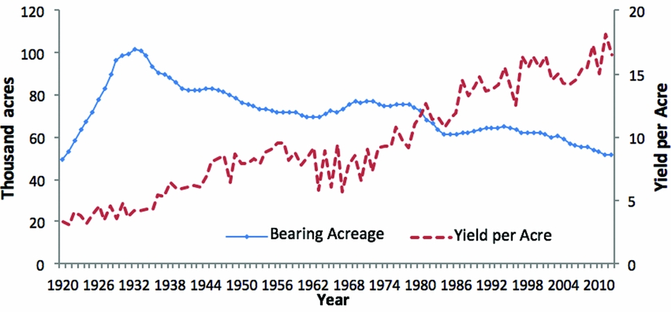
Figure A1. Farm-Level U.S. Pear Production (source: U.S. Department of Agriculture, National Agricultural Statistics Service, 2016)
Once tree fruit is harvested, it is allocated to either the fresh or processed market. Pears that satisfy quality standards go to the fresh market, which historically commands higher prices. Contractually committed and residual pears go to the processed market. About 39% of U.S. pears entered the fresh market in 1980, but this increased to 65% by 2012 (Figure A2).
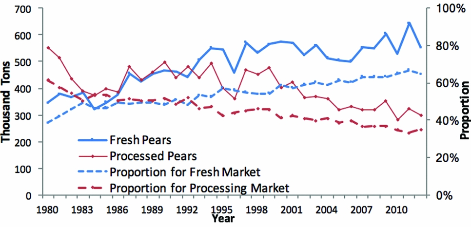
Figure A2. Allocation of U.S. Pears to Fresh and Processed Markets (source: U.S. Department of Agriculture, National Agricultural Statistics Service, 2016)
Per capita consumption of fresh and processed pears declined from 7.24 pounds in 1980 to 4.83 pounds in 2012. The declining trend is especially strong for processed pears. The U.S. consumption in 2012 for fresh pears was 2.78 pounds per capita and for processed pears was 2.05 pounds per capita fresh equivalent weight. In 1980, the per capita consumption was 2.60 pounds for fresh pears and 4.64 pounds for processed pears (USDA, Economic Research Service, 2016; Figure A3).
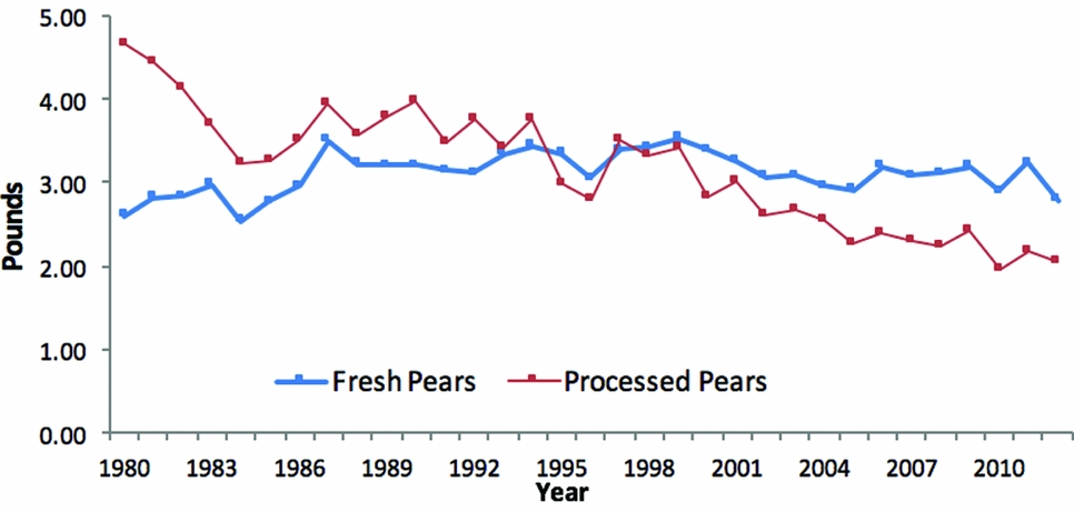
Figure A3. Per Capita Consumption of Fresh and Processed Pears in the United States (source: U.S. Department of Agriculture, Economic Research Service, 2016)
The United States is a net exporter of fresh pears. The United States exported 211,248 tons in 2012 compared with 81,704 tons in 1989. According to USDA, Foreign Agricultural Service (2016), U.S. fresh pears are imported by more than 50 countries, the largest markets being Canada, Mexico, Brazil, and Russia. Although the United States is a major supplier of pears in the domestic market, pears from Argentina, Chile, South Korea, and other nations also enter the market. Zhang, Marsh, and Schotzko (Reference Zhang, Marsh and Schotzko2007) show that the majority of imported pears enter the U.S. market during the February to May domestic production off-season.
Historically, the United States has also been a net exporter of processed pears, but it became a net importer after 2000. By 2012, the United States imported processed pears from about 10 countries, though approximately 90% are from China. As for exports of processed pears, the United States ships primarily to Canada and Mexico, which together account for 80% of U.S. processed pear exports since 2007 (Figure A4).
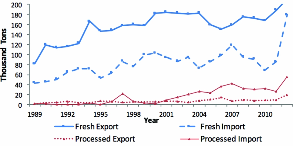
Figure A4. U.S. Exports and Imports of Fresh and Processed Pears (source: U.S. Department of Agriculture, Foreign Agricultural Service, 2016)
Appendix B: Equilibrium Displacement Model and Welfare Analysis Equations
Equilibrium Displacement Model
A numerical solution for the partial equilibrium model is facilitated by a total logarithmic differential version of the model equations. This is conceptually and numerically advantageous because the differential version gives the elasticities of the model.
The farm-level demand for fresh fruit is FD f, t = FPf (pF f, t , FSt ). The total logarithmic differential equation is as follows:
 $$\begin{equation}
d\ln F{D_{f,t}} = \varepsilon _f^Fd\ln p_{f,t}^F + {\textstyle{{\left( {{{\partial F{P_{f,t}}}
/ {F{D_{f,t}}}}} \right)} \over {\left( {{{\partial F{S_t}}
/ {F{S_t}}}} \right)}}}d\ln F{S_t},
\end{equation}$$
$$\begin{equation}
d\ln F{D_{f,t}} = \varepsilon _f^Fd\ln p_{f,t}^F + {\textstyle{{\left( {{{\partial F{P_{f,t}}}
/ {F{D_{f,t}}}}} \right)} \over {\left( {{{\partial F{S_t}}
/ {F{S_t}}}} \right)}}}d\ln F{S_t},
\end{equation}$$
where $\scriptstyle{\varepsilon _f^F = \frac{{d\ln F{D_{f,t}}}}{{d\ln p_{f,t}^F}}}$
is the own-price elasticity of farm-level demand for fresh fruit, and ε =
$\scriptstyle{\varepsilon _f^F = \frac{{d\ln F{D_{f,t}}}}{{d\ln p_{f,t}^F}}}$
is the own-price elasticity of farm-level demand for fresh fruit, and ε = $\scriptstyle{\frac{{{\raise0.5ex\hbox{$\scriptstyle {\partial F{P_{f,t}}}$} \kern-0.1em\left/\vphantom{A_P}\right.\kern-0.15em \lower0.25ex\hbox{$\scriptstyle {F{D_{f,t}}}$}}}}{{{\raise0.5ex\hbox{$\scriptstyle {\partial F{S_t}}$} \kern-0.1em\left/\vphantom{A_P}\right.\kern-0.15em \lower0.25ex\hbox{$\scriptstyle {F{S_t}}$}}}}}$
measures the change in the proportion of total production and its impact on the allocation to the fresh market. The total logarithmic differential equation derived from FD
p, t
= FSt
− FD
f, t
is as follows:
$\scriptstyle{\frac{{{\raise0.5ex\hbox{$\scriptstyle {\partial F{P_{f,t}}}$} \kern-0.1em\left/\vphantom{A_P}\right.\kern-0.15em \lower0.25ex\hbox{$\scriptstyle {F{D_{f,t}}}$}}}}{{{\raise0.5ex\hbox{$\scriptstyle {\partial F{S_t}}$} \kern-0.1em\left/\vphantom{A_P}\right.\kern-0.15em \lower0.25ex\hbox{$\scriptstyle {F{S_t}}$}}}}}$
measures the change in the proportion of total production and its impact on the allocation to the fresh market. The total logarithmic differential equation derived from FD
p, t
= FSt
− FD
f, t
is as follows:
 $$\begin{equation}
d\ln F{D_{p,t}} = \frac{{F{S_t}}}{{F{D_{p,t}}}}d\ln F{S_t} - \frac{{F{D_{f,t}}}}{{F{D_{p,t}}}}d\ln F{D_{f,t}}.
\end{equation}$$
$$\begin{equation}
d\ln F{D_{p,t}} = \frac{{F{S_t}}}{{F{D_{p,t}}}}d\ln F{S_t} - \frac{{F{D_{f,t}}}}{{F{D_{p,t}}}}d\ln F{D_{f,t}}.
\end{equation}$$
Total logarithmic differentiation of the market margin equation between farm-level and wholesale (pF i = pi W − MMF i ) and between retail and wholesale (pR i = pi W + MMR i ) gives the following:
 $$\begin{equation}
d\ln p_i^W = \frac{{p_i^F}}{{p_i^W}}d\ln p_i^F + \frac{{MM_i^F}}{{p_i^W}}d\ln MM_i^F\,{\rm{and}}
\end{equation}$$\\
$$\begin{equation}
d\ln p_i^W = \frac{{p_i^F}}{{p_i^W}}d\ln p_i^F + \frac{{MM_i^F}}{{p_i^W}}d\ln MM_i^F\,{\rm{and}}
\end{equation}$$\\
 $$\begin{equation}
d\ln p_i^R = \frac{{p_i^W}}{{p_i^R}}d\ln p_i^W + \frac{{MM_i^R}}{{p_i^R}}d\ln MM_i^R.
\end{equation}$$
$$\begin{equation}
d\ln p_i^R = \frac{{p_i^W}}{{p_i^R}}d\ln p_i^W + \frac{{MM_i^R}}{{p_i^R}}d\ln MM_i^R.
\end{equation}$$
 $$\begin{equation}
d\ln Q_i^D = d\ln pop + {\varepsilon _f}d\ln {p_f} + {\varepsilon _p}d\ln {p_p} + {\varepsilon _I}d\ln I + d\ln z,
\end{equation}$$
$$\begin{equation}
d\ln Q_i^D = d\ln pop + {\varepsilon _f}d\ln {p_f} + {\varepsilon _p}d\ln {p_p} + {\varepsilon _I}d\ln I + d\ln z,
\end{equation}$$
where $\scriptstyle{{\varepsilon _f} = \frac{{d\ln Q_i^D}}{{d\ln {p_f}}}}$
is the elasticity of retail demand for fruit i with respect to retail fresh fruit price,
$\scriptstyle{{\varepsilon _f} = \frac{{d\ln Q_i^D}}{{d\ln {p_f}}}}$
is the elasticity of retail demand for fruit i with respect to retail fresh fruit price, $\scriptstyle{{\varepsilon _p} = \frac{{d\ln Q_i^D}}{{d\ln {p_p}}}}$
is the elasticity of retail demand for fruit i with respect to retail processed fruit price, and
$\scriptstyle{{\varepsilon _p} = \frac{{d\ln Q_i^D}}{{d\ln {p_p}}}}$
is the elasticity of retail demand for fruit i with respect to retail processed fruit price, and $\scriptstyle{{\varepsilon _I} = \frac{{d\ln Q_i^D}}{{d\ln I}}}$
is the income elasticity. Taking total logarithmic differentiation of the exported fruit Ei
= fEx
i
(pW
i
− ci
SPS
) · γ
ei
gives the following:
$\scriptstyle{{\varepsilon _I} = \frac{{d\ln Q_i^D}}{{d\ln I}}}$
is the income elasticity. Taking total logarithmic differentiation of the exported fruit Ei
= fEx
i
(pW
i
− ci
SPS
) · γ
ei
gives the following:
 $$\begin{equation}
d\ln E_i^{} = \varepsilon _i^{es}{\left( {p_i^e - c_i^{SPS}} \right)^{ - 1}}\left( {p_i^ed\ln p_i^e - dc_i^{SPS}} \right) + d\gamma_{e_i}.
\end{equation}$$
$$\begin{equation}
d\ln E_i^{} = \varepsilon _i^{es}{\left( {p_i^e - c_i^{SPS}} \right)^{ - 1}}\left( {p_i^ed\ln p_i^e - dc_i^{SPS}} \right) + d\gamma_{e_i}.
\end{equation}$$
Fruit import demand is ${M_i} = f_i^{{\mathop{\rm Im}\nolimits} }(p_i^W - {t_{{m_i}}})$
. The logarithmic differentiation of that is as follows:
${M_i} = f_i^{{\mathop{\rm Im}\nolimits} }(p_i^W - {t_{{m_i}}})$
. The logarithmic differentiation of that is as follows:
 $$\begin{equation}
d\ln M_i^{} = \varepsilon _i^{md}{\left( {p_i^W - t_{m_i}} \right)^{ - 1}}\left( {p_i^Wd\ln p_i^W - dt_{m_i}} \right),
\end{equation}$$
$$\begin{equation}
d\ln M_i^{} = \varepsilon _i^{md}{\left( {p_i^W - t_{m_i}} \right)^{ - 1}}\left( {p_i^Wd\ln p_i^W - dt_{m_i}} \right),
\end{equation}$$
where ε md i is the own-price elasticity of imported fruit i. Domestic retail-level supply is QSi = FSi + Mi − Ei . Total logarithmic differentiation gives the following:
 $$\begin{equation}
\begin{array}{@{}l@{}} d\ln Q{S_i} = \frac{{FS_i^{}}}{{Q{S_i}}}d\ln FS_i^{} + \frac{{M_i^{}}}{{Q{S_i}}}\left[ {\varepsilon _i^{md}{{\left( {p_i^W - t_{m_i}} \right)}^{ - 1}}\left( {p_i^Wd\ln p_i^W - dt_{m_i}} \right)} \right]\\
\qquad\qquad\quad- \frac{{E_i^{}}}{{Q{S_i}}}\left[ {\varepsilon _i^{es}{{\left( {p_i^e - c_i^{SPS}} \right)}^{ - 1}}\left( {p_i^ed\ln p_i^e - dc_i^{SPS}} \right) + d\gamma_{e_i}} \right]. \end{array}.
\end{equation}$$
$$\begin{equation}
\begin{array}{@{}l@{}} d\ln Q{S_i} = \frac{{FS_i^{}}}{{Q{S_i}}}d\ln FS_i^{} + \frac{{M_i^{}}}{{Q{S_i}}}\left[ {\varepsilon _i^{md}{{\left( {p_i^W - t_{m_i}} \right)}^{ - 1}}\left( {p_i^Wd\ln p_i^W - dt_{m_i}} \right)} \right]\\
\qquad\qquad\quad- \frac{{E_i^{}}}{{Q{S_i}}}\left[ {\varepsilon _i^{es}{{\left( {p_i^e - c_i^{SPS}} \right)}^{ - 1}}\left( {p_i^ed\ln p_i^e - dc_i^{SPS}} \right) + d\gamma_{e_i}} \right]. \end{array}.
\end{equation}$$
Retail-level market-clearing conditions are given by equation QDi + Ei = FSi + Mi . The total logarithmic differentiation equation is then:
 $$\begin{equation}
\begin{array}{@{}l@{}} d\ln pop + {\varepsilon _f}d\ln {p_f} + {\varepsilon _p}d\ln {p_p} + {\varepsilon _I}d\ln I + d\ln z\\
\quad = \frac{{FS_i^{}}}{{Q{S_i}}}d\ln FS_i^{} + \frac{{M_i^{}}}{{Q{S_i}}}\left[ {\varepsilon _i^{md}{{\left( {p_i^W - t_{m_i}} \right)}^{ - 1}}\left( {p_i^Wd\ln p_i^W - dt_{m_i}} \right)} \right]\\ \qquad - \frac{{E_i^{}}}{{Q{S_i}}}\left[ {\varepsilon _i^{es}{{\left( {p_i^e - c_i^{SPS}} \right)}^{ - 1}}\left( {p_i^ed\ln p_i^e - dc_i^{SPS}} \right) + d\gamma_{e_i}} \right]. \end{array}
\end{equation}$$
$$\begin{equation}
\begin{array}{@{}l@{}} d\ln pop + {\varepsilon _f}d\ln {p_f} + {\varepsilon _p}d\ln {p_p} + {\varepsilon _I}d\ln I + d\ln z\\
\quad = \frac{{FS_i^{}}}{{Q{S_i}}}d\ln FS_i^{} + \frac{{M_i^{}}}{{Q{S_i}}}\left[ {\varepsilon _i^{md}{{\left( {p_i^W - t_{m_i}} \right)}^{ - 1}}\left( {p_i^Wd\ln p_i^W - dt_{m_i}} \right)} \right]\\ \qquad - \frac{{E_i^{}}}{{Q{S_i}}}\left[ {\varepsilon _i^{es}{{\left( {p_i^e - c_i^{SPS}} \right)}^{ - 1}}\left( {p_i^ed\ln p_i^e - dc_i^{SPS}} \right) + d\gamma_{e_i}} \right]. \end{array}
\end{equation}$$
By solving the single fruit equilibrium, we can then derive retail-level fresh and processed price based on the retail-level market-clearing conditions and markup equations. Feeding those prices into the model equations given previously yields the quantities at the farm and retail levels.
The list of endogenous variables is as follows: pF f, t , p p, t F , pW f, t , p p, t W , pR f, t , p p, t R , E f, t , E p, t , M f, t , M p, t , QD f, t , QD p, t , FS t , FD f, t , FD p, t . The list of exogenous variables and their values may be found in Table 1 of the main text.
Welfare Analysis Equations
We measure producer and intermediary surplus by the quasi returns to capital and management, which are a constant fraction of total revenue. That is, the quasi returns to capital and management are the constant share of revenue not going to labor and other expenses. The change to producer surplus in year t is the difference between the quasi returns to capital and management in the shock scenario to the baseline:
 $$\begin{equation}
\Delta P{S_{i,t}} = rate_i^{} \cdot TR_{i,t}^S - rate_i^{} \cdot TR_{i,t}^{\rm Baseline},
\end{equation}$$
$$\begin{equation}
\Delta P{S_{i,t}} = rate_i^{} \cdot TR_{i,t}^S - rate_i^{} \cdot TR_{i,t}^{\rm Baseline},
\end{equation}$$
where i is the index for fresh and processed pears; ratei is the fraction of total revenue that goes to growers; total revenue for growers in year t is TR i, t = pF i, t · FS i, t ; TRS i, t and TR Baseline i, t are the total revenue under shock S and under the baseline; pF i, t is the farm price for i at year t; and FS i, t is the quantity for i at year t. The values we use for rate are given in Table 1 in the main text.
To get the net present value of the change in welfare for producers, we use a 4% discount on the year-to-year welfare calculations from equation (A-10) for 60 years—that is,
 $$\begin{equation}
NPS_i^S = \sum\limits_{t = 1}^{60} {\frac{{\Delta P{S_{i,t}}}}{{{{(1 + 0.04)}^{t - 1}}}}} .
\end{equation}$$
$$\begin{equation}
NPS_i^S = \sum\limits_{t = 1}^{60} {\frac{{\Delta P{S_{i,t}}}}{{{{(1 + 0.04)}^{t - 1}}}}} .
\end{equation}$$
Because 4% is just the discount, it is a scaling factor. Thus, it controls the quantitative level of welfare, but not the qualitative result. We use the same calculation for change to intermediary surplus for fresh and processed pears by updating the values accordingly.
Domestic consumer benefits associated with the shock are calculated as the change in the area below the domestic demand curve, reflecting the effects of both price and quantity changes. Per capita consumer welfare is $d\ln y = \varepsilon d\ln p \Rightarrow \frac{{dy}}{y} = \varepsilon \frac{{dp}}{p}$
. Integrating both sides gives the following:
$d\ln y = \varepsilon d\ln p \Rightarrow \frac{{dy}}{y} = \varepsilon \frac{{dp}}{p}$
. Integrating both sides gives the following:
 $$\begin{equation}
\begin{array}{@{}l@{}} \int {\frac{{dy}}{y}} = \int {\varepsilon \frac{{dp}}{p}} + c \Rightarrow \ln y = \varepsilon \ln p + c \Rightarrow y = {e^{\ln {p^\varepsilon } + c}} \Rightarrow y = {p^\varepsilon }{e^c} \Rightarrow y = {p^\varepsilon }c\\ c = y/{p^\varepsilon }. \end{array}
\end{equation}$$
$$\begin{equation}
\begin{array}{@{}l@{}} \int {\frac{{dy}}{y}} = \int {\varepsilon \frac{{dp}}{p}} + c \Rightarrow \ln y = \varepsilon \ln p + c \Rightarrow y = {e^{\ln {p^\varepsilon } + c}} \Rightarrow y = {p^\varepsilon }{e^c} \Rightarrow y = {p^\varepsilon }c\\ c = y/{p^\varepsilon }. \end{array}
\end{equation}$$
Per capita consumer surplus is $\int_p^{p^{\prime}} {ydp} = c\int_p^{p^{\prime}} {{p^\varepsilon }dp} = c\frac{{{p^{\varepsilon + 1}}}}{{\varepsilon + 1}}| {_p^{p^{\prime}}} $
, where p′ is the price in the shock scenario. Then total consumer surplus is this per capita surplus times population: TCS = per capita CS × population. The period t change in consumer surplus between shock S and baseline is ΔTCSt
= TCSS
t
− TCS
Baseline
t
. The net present value of change in consumer surplus is calculated using the discount rate of 4% over 60 years:
$\int_p^{p^{\prime}} {ydp} = c\int_p^{p^{\prime}} {{p^\varepsilon }dp} = c\frac{{{p^{\varepsilon + 1}}}}{{\varepsilon + 1}}| {_p^{p^{\prime}}} $
, where p′ is the price in the shock scenario. Then total consumer surplus is this per capita surplus times population: TCS = per capita CS × population. The period t change in consumer surplus between shock S and baseline is ΔTCSt
= TCSS
t
− TCS
Baseline
t
. The net present value of change in consumer surplus is calculated using the discount rate of 4% over 60 years:
 $$\begin{equation}
NCS_i^S = \sum\limits_{t = 1}^{60} {\frac{{\Delta TC{S_{i,t}}}}{{{{(1 + 0.04)}^{t - 1}}}}} ,
\end{equation}$$
$$\begin{equation}
NCS_i^S = \sum\limits_{t = 1}^{60} {\frac{{\Delta TC{S_{i,t}}}}{{{{(1 + 0.04)}^{t - 1}}}}} ,
\end{equation}$$
where fresh and processed pears are indexed as i.


 Open access