


1. Introduction
This is one of a series of papers on the elastic properties of sea ice. Previous reports are Reference Pounder and StalinskiPounder and Stalinski (1961[b]), Reference LanglebenLangleben (1962), and Reference Langleben, Pounder and KingeryLangleben and Pounder (1963), the last paper including a review of earlier work. The observations reported here were made in April–May 1962 on the floating sea ice cover at lat. 78° 42′ N., long. 104° 06′ W. near lsachsen, Ellcf Ringnes Island, N.W.T. Other investigations made during this expedition are given in Reference Langleben and PounderLangleben and Pounder (1964).
Two types of ice were available, namely polar ice of unknown age but more than two years old and “biennial” ice which had started to form in the fall of 1960 some twenty months prior to the observations.
2. Methods
Most of the observations were made on 6-in. (15.2-cm.) sections of cores extracted from the ice cover with a SIPRE core drill which cuts out cylinders of diameter 3 in. (7.6 cm.). Full details of the sonic techniques used are given in the references above. Briefly, barium titanatc transducers were attached to both ends of the sample and the input transducer was excited with repetitive pulses having a sharp leading edge. The transit time for a pulse was measured by comparing it with a calibrated time delay in the DuMont Type 326 generator which supplied triggers for both the input pulse to the ice and the sweep for the cathode ray oscilloscope on which the received pulse was displayed. The resonant frequency of the input transducer was sufficiently high that the wave-length of the longitudinal waves was less than to per cent of the diameter of the sample so that it could be considered to be an infinite medium. Measurement of transit time for a known length thus gave the bulk velocity c B, with an estimated accuracy of 1.5 per cent or better.
The equation for the bulk velocity involves both Young’s modulus E and Poisson’s ratio σ 0 so that two independent measurements are needed. In principle, measurement of the resonant frequencies of the ice sample will give sufficient data. For this measurement the input transducer is driven by a sinusoidal oscillator which is swept slowly over the range from about 8 to 80 kc. sec.−1, resonant frequencies being detected by increases in the amplitude of the output transducer. This tedious method gives ambiguous results because the large number of spurious resonances found makes identification of the correct frequencies difficult. Reference Langleben, Pounder and KingeryLangleben and Pounder (1963) gave the results of a number of resonant measurements of this type on ice samples of widely differing brine content y from covers of both annual and polar ice. They concluded tentatively that σ 0 is almost independent of salinity, temperature, and type of sea ice and gave a value of σ 0 = 0.295.
In the present experiment, resonant frequencies were measured for eight ice samples, from vertical cores of polar ice and both vertical and horizontal cores of biennial ice. The result was σ 0 = 0.299±0.007. The uncertainty quoted is simply the maximum observed deviation from the average; systematic error, which is all too likely with this method, could not be estimated.
Supporting observations on the core samples were made in the usual way. Most of the ice samples (about 80 per cent of those used for measurements) were melted after the mechanical and acoustical tests and their salinities found by titration. The density profiles of the two types of ice were found by measurements on one core each of polar and biennial ice, in which the mass of a sample was found by weighing and its volume by the amount of n-heptane it displaced in a calibrated vessel. The crystal structure of each type of ice was observed by photographing thin vertical and horizontal sections of a core between crossed polaroids, at frequent intervals of depth below the surface.
Some simple seismic measurements were also made on the biennial ice cover, using a seismic hammer. With this instrument, the seismic shock is generated by striking the ice smartly with a heavy sledge hammer. Attached to the hammer is a microswitch which is actuated by the blow and transmits the “shot instant” by wire to the timing device, acting to trigger a scale-of-two counter which was accurate to 0.25 msec. A finite time later the seismic waves reach the geophone, which is also connected to the counter. The first arrival of the seismic wave (i.e. the leading edge) serves to stop the counter and the time taken for the waves to travel from “shot point” to geophone plant are registered. By striking different vertical faces of a rectangular pit in the ice, the waves propagated in the direction of the geophones may be either predominantly compressional or shear and may be detected by suitably oriented geophones.
Measurements were made over path lengths of 40, 80 and 120 m., which were chained off. At each detection point, the snow was shovelled off the ice and two horizontal-component geophones were firmly planted in intimate contact with the ice and then covered with snow to reduce wind noise. The axis of one pointed towards the point of impact to receive the compressional wave when the ice was struck in that direction, the other was oriented at right angles to this direction so as to detect the shear wave. Each geophone in turn was connected to the counter. Sufficient hammer blows were struck to obtain about six identical counter readings of the time of first arrival at each geophone plant. Spurious readings sometimes resulted when vibrations other than those generated by the hammer were detected by the geophone and tripped the counter prematurely. On the other hand, at low amplifier sensitivity or for a weak hammer blow, it was sometimes possible to observe longer transit times.
The shear velocity c s was calculated directly from t s, the time taken for the shear waves to travel over a given distance. (The shear wave was too weak for measurement at the range of 120 m.) The compressional wave propagated in a floating ice sheet at distances large compared with ice thickness (i.e. for long wave-lengths) is the longitudinal plate wave. It travels more slowly than the bulk compressional wave. The bulk velocity c B can, however, be calculated indirectly from the transit time t p of the longitudinal plate waves using the expression

The calculation of Poisson’s ratio and Young’s modulus then follows from

and
3. Results
Salinity
Eighteen cores were extracted vertically from the polar ice, all from within an area of radius 4 ft. (1.2 m.). Five of these cores were analysed in detail for salinity. Four of the eleven vertical cores of biennial ice (from an area of radius 3 ft. (0.9 m.)) were analysed similarly. Separate salinity tests were made on the horizontal cores. Average salinity profiles for the two types of ice are shown in Figure 1. Deviations of measured salinities from these curves were usually less than 0.1‰ although there were a few deviations up to 0.2‰. It will be seen that there is only a slight difference in salinity of the two types, the polar ice being more saline, and that the upper 6 ft. (1.8 m.) of either type of ice cover has a salinity of 1‰ or less. The temperatures of the icc samples at the time of measurement ranged from −3° to −12° C., and the combination of low salinity and narrow temperature range gave a very limited range of values for brine content with almost all values of v being below 10‰.
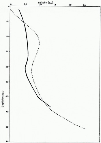
Fig. 1. Average salinity profiles of polar ice (dashed line) and biennial ice (solid line) in the ice cover near Irachsen, May 1962
Density
As has been pointed out in earlier papers, the density of a given sheet of sea ice is almost constant. In this case the polar ice showed no systematic variation in density with depth, the average being 0.894± 0.006 g. cm.−3. The density of the biennial ice was constant at 0.902±0.003 g. cm.−3 at depths below 30 in (76 cm.). The upper layer of this ice was slightly less dense. On the basis of two measurements, a linear interpolation for the specific gravity of 0.854+1.62×10⁻² d, where d is the depth in inches below the ice surface, was used in calculations on the top 30 in. (76 cm.) of the biennial ice.
Crystal structure
The cover of biennial ice started to form in September 1960 and, from the evidence of observers at Isachsen in the summer of 1961, it remained shore-fast up to the time of this work. This was borne out by the absence of pressure ridging. The snow cover was heavy, and from examination of the snow–ice interface it was clear that no surface melting of the ice had taken place. The crystal structure resembled closely that of annual sea ice; the surface layer consisted of many small, randomly oriented crystals but below about 1 ft. (30 cm.) the crystals were large (typically 2–5 cm. across and many centimeters in vertical height). There was a tendency for the crystal size to increase with depth, but in the bottom part (sections from 6 to 8 ft. (1.8 to 2.4 m.) in depth) there was an increase in the number of small crystals in a section. This tendency was noted in annual ice by Reference Pounder and StalinskiPounder and Stalinski (1961[a]). In this case it may represent new growth during the winter of 1961–62.
The polar ice was more uniform than the biennial. The average crystal size was smaller and there was no systematic change in the crystals with depth. Because of the gently rounded hummocks of the polar ice it is a reasonable guess that this floe was over five years old. Presumably it had therefore gone through several cycles of surface melting and growth on the bottom. The crystal sections gave no evidence of the alternating annual layers reported by Reference CherepanovCherepanov (1957).
Young’s modulus
Sonic measurements were made on three categories of ice, 98 samples from vertical cores of polar ice, 99 samples from vertical cores of biennial ice, and 21 samples from horizontal cores of biennial ice. Using a fixed value of σ 0 (0.295) in all calculations, Young’s modulus was evaluated for each sample from the length, transit time, and density, and the brine content from the salinity and temperature (using the table in Reference AssurAssur, 1958). Within each category the values obtained were sorted in order of increasing brine content, and then both v and E were averaged in groups of about ten observations. The results are given in Table I and plotted in Figure 2. The line in Figure 2 is the empirical equation found by Langleben for annual sea ice, namely
Table I. Summary of Observations
E is in units of 1010 dyne cm−2, ν in ‰. E cal is based on equation (1). ΔE = E cal−E obs. Number of observations averaged in each group = n


Fig. 2. Values of Young’s modulus. Data are coded as follows: solid circles (polar ice), squares (biennial ice—vertical cores), and crosses (biennial ice—horizontal cores). The line is the empirical variation of E with brine content for annual sea ice
where E is in units of 1010 dyne cm.−2 and ν is in ‰. This equation was deduced from measurements made at Thule on both natural sea ice and on sea ice artificially thickened by flooding the surface with sea-water. The resulting high freezing rates gave very high brine contents so that equation (1) is based on observations with 0<ν<85‰. Another possible comparison is with the result found by Pounder for polar ice in summer, namely
in the same units as (1). The range of ν values observed was 0–75‰. but the possible errors in ν were much larger because of its rapid change with temperature in the 0° to −5° C. region.
As mentioned above, the range in y in the Isachsen experiments was only 0–10‰, too narrow a range to make useful a least-squares analysis of the data to produce a functional relation between E and ν. A comparison with the results predicted by equations (1) and (2) is more significant. All the observed values of E were slightly lower than predicted by (1) and much higher than given by (2). In Table I the comparison is made with values calculated from (1). Vertical cores from both polar and biennial ice gave values of Young’s modulus averaging 3.6 per cent lower than those for annual sea ice of similar brine content. The comparable figure for the samples of ice cut horizontally was 4.7 per cent lower.
Seismic measurements
Table II shows the results of about six observations at each of the three ranges. The results for the longest path length were calculated assuming the value of c s measured for the shorter ones.
Table II. Seismic Measurements of Biennial Ice

The possible or percentage possible errors are indicated in the 40 m. range column of Table II, assuming that the error in measurement of range is negligible. The percentage errors in σ 0 and E at ranges of 80 and 120 m. are less than those at 40 m. The twofold increase in travel time in going from a range of 40 m. to 80 m. for both the shear wave and the longitudinal plate wave rules out the possibility of systematic error.
It will be noted that the values of Poisson’s ratio in Table II are some 15 per cent lower than the value of 0.295 from previous work, and that the values of Young’s modulus are 25 per cent lower than the value of 9.65 predicted by equation (1) for ice of average brine content of 10‰. This may he compared with E values 3.6 per cent lower from the sonic tests on vertical cores described above, although the comparison is not quite apt because of the differences in the two types of tests. In the sonic measurements, waves were propagated along the long dimension of the ice crystals, i.e. in the direction which was vertical in the ice cover, whereas in the seismic work the direction of wave propagation was essentially horizontal.
4. Discussion
The sonic measurements on small ice samples showed no significant difference between biennial and polar ice, and the differences between them in density, salinity, and crystal structure were quite minor. It appears that sea ice which has gone through a summer, even one in which no surface melting occurs (as was the case at Isachsen in 1961), has lost most of its salt and might as well be classed as polar ice for most purposes. It should be noted, however, that an appreciable difference was observed in the ultimate tensile strength of the two types of ice (Reference Langleben and PounderLangleben and Pounder, 1964).
Results of the small-scale tests on vertical cores confirmed that Young’s modulus for cold polar ice is slightly lower than it is for annual ice, a result suggested earlier by the authors on the basis of very limited evidence.
The discrepancy betwcen the results of the seismic tests and the measurements on the horizontal cores is puzzling, since both involve wave propagation transverse to the long dimensions of the ice crystals. The seismic wave was travelling in slightly warmer ice. In situ ice temperatures were not recorded, but even if the coldest part of the ice cover was as warm as −3° C. and its salinity was 1‰ this would correspond to ν = 16.2‰ and E = 9.43×10¹⁰ dyne cm.−2 from (1), which is far from the results given in Table II. Reference Brown and KingeryBrown (1963) has recently reported an exhaustive set of tests on sea-ice sheets at various localities using standard seismic techniques. He too finds that values of Young’s modulus for these large-scale tests are considerably lower than those associated with small-sample testing.
This type of discrepancy is quite common in measurements of ultimate strengths. Small-scale tests (such as ring-tensile ones) almost invariably give higher mechanical strengths than large-scale ones (e.g. fracture of large cantilever beams). It is usual to attribute this to a random distribution of flaws in ice, and possibly some such mechanism is responsible for the seismic results. Against this, it should be noted that the value of c S appears quite normal. It is the low values of c B which are responsible for the low values of E. Since the measurements are made on first arrival, i.e. the wave which has found the shortest path, it is difficult to see why macroscopic flaws or fractures, or microscopic flaws such as intercrystalline boundaries or brine pockets should act differentially on compressional and shear waves.
Acknowledgements
The assistance on this expedition of Mr. J. R. Addison, Mr. F. M. Boyce, and Dr. P. Schwerdtfeger of the Ice Research Project is recorded with thanks. We arc indebted to the Pacific Naval Laboratory and the Defence Research Northern Laboratory for the loan of equipment, and to the Royal Canadian Air Force and the Polar Continental Shelf Project for logistic aid. The work was supported by the Defence Research Board of Canada under D.D.P. Contract GC.69–200004.


