

1. Introduction
When engineering works are planned close to a glacier it would be a great help to have a reliable method of predicting the future behaviour of the glacier. No such method at present exists. But it is possible, in certain circumstances, to predict what the glacier response would be to a given variation in its mean mass balance. If plausible limits are then set to the possible future variation in mass balance, corresponding limits may be set to the variations of the glacier. Variations in the length caused by other factors than changes in the mass balance are not covered by this procedure, and therefore glacier surges are outside its scope. The strongest indication that an individual glacier is capable of and has experienced surges is the presence of folded moraines. They are not present on the glacier which is the subject of this paper, and there is no reason to believe that it has surged in the past.
The calculations to be described were done to see whether Berendon Glacier (Fig. 1), in the Coast Mountains of British Columbia, Canada, was likely to advance sufficiently in the next 40 years or so to be a danger to the mining installations of the Granduc Operating Co.Footnote * They are reported here because they illustrate a method that may be useful in similar problems elsewhere. The Berendon Glacier (lat. 56° 15′ N., long. 130° 05′ W.), which covers an area of 33 km2 between altitudes of about 2400 m and 655 m, has two main branches that join together at an altitude of 1100 m. It has not been extensively studied, and in this respect it differs from the other glaciers to which this type of theory has been applied, namely South Cascade Glacier, Washington, U.S.A. and Storglaciären, Kebnekaise, Sweden. The data for these last two glaciers were of high quality and the results of the computations were correspondingly reliable; in contrast, the data used for Berendon Glacier necessarily involved a good deal of guesswork. In spite of this the results are thought to be significant, and certainly better than estimates of the likely behaviour of the glacier based on no theory at all.

Fig. 1. Berendon Glacier, Coast Mountains of British Columbia, Canada. The tunnel portal, al the point marked X in lower left corner, was 19 m above and 180 m horizontally from the edge of the ice in 1963. Photograph taken by Austin S. Post on 8 August 1961
2. Procedure
The theory used, which is concerned only with changes in the glacier that are small compared with the overall dimensions, is developed in the five papers (Reference NyeNye, 1960, Reference Nye1963[a], Reference Nye1963[b], Reference Nye1965[a], Reference Nye1965[b]), of which Reference NyeNye (1963[b]) is the most relevant for our present purpose and is more or less self-contained. The glacier is characterized by three functions B 0(x),c 0(x),D 0(x), where x is a coordinate denoting distance down the glacier, the functions being respectively the width of the glacier in a datum state, the velocity of kinematic waves multiplied by B 0, and the diffusivity of kinematic waves multiplied by B 0. To estimate these functions for the Berendon Glacier we used the same procedure as that already fully described for South Cascade Glacier (Reference NyeNye, 1963[b]) and Storglaciären (Reference NyeNye, 1965[a]), the only difference in this case being the paucity of the observational data.
There are three topographical maps of Berendon Glacier (scale 1: 1200, contour interval 20 ft (6·1 m)), based on aerial photographs taken in 1949, 1956 and 1963 by Hunting Survey Corporation, Vancouver, B.C. The earliest one does not cover the region of the terminus, and none of them covers the upper reaches of the accumulation area. The data presented in Table I are based on the 1963 map, extended for the upper reaches of the glacier by an approximate topography taken from Sheet 104B, “National Topographic Series” of Canada (scale 1: 250000). The coordinate x (at intervals of Δx = 600 m) was measured along median lines of the two major and several minor ice streams of Berendon Glacier. The widths of each of the individual streams, at the same x, were measured roughly along contour lines and added to obtain the function B 0(x) for the whole glacier. Since the variation of altitude with x is different in each tributary, the mean altitude z over each interval Δx was determined by weighting the altitudes of the tributary strips according to their widths. The variation of the mass balance a with x was then estimated from the known variation with altitude of the mass balances of eight other glaciers along the coast between Washington and Alaska (Reference Meier and PostMeier and Post, 1962). Combined with the values of B 0, the chosen function a(x) gave a negative mean mass balance, as was likely to be true in 1963. A uniform addition of +15 cm/year at all heights was made to establish the function a 0(x) giving a zero mean mass balance as required for the datum state.

An idealized steady-state datum glacier was thus set up which had a length approximately equal to that of the real glacier in 1963. The bedrock topography is not known and had to be inferred from cross-sections of the valleys in the lower part of the glacier, and estimated in the upper part. The annual discharge volumes q 0 and the ice velocities u 0 in this datum glacier, implied by the assumed mass-balance curve and the assumed cross-sectional areas of the glacier, were reasonable but could not be checked against actual measurements. It is clear that the resulting functions B 0(x), c 0(x), D 0(x) for Berendon Glacier are very approximate. When calculating the response of the terminus it is fortunately not necessary that the functions should be known in detail in the upper reaches of the glacier, for the response is the result of an integration down the length of the glacier. But it is important that the value of c 0(x) at the terminus itself (x = L) should be accurately known. For example, the response of the terminus to a long-term change in mean mass balance, a 1, is given by

where h 1, is the thickening at the terminus. The integral is simply the area of the glacier. An error in c 0(L) thus leads directly to an equal percentage error in the calculated response. We estimated c 0(L) as between 0·5×104 and 1·0×104 m2/year−1 with the most likely value as 0·7×104 m2/year−1. If the object had been to compute the response of the terminus, this uncertainty in c 0(L) would have been a serious source of error. There would also have been difficulties in interpreting the theory in a region where the width of the glacier is changing by relatively large amounts. But, in fact, the threat of the glacier to the installations was not at the terminus itself (x = 8 790 m) but at a point 800 m further up-glacier (x = 7 990 m); at this position the portal of the mine workings (marked by a cross in Figure 1) lay 19 m above the 1963 ice level. The width in this region is relatively well defined, and, as we verified by computation, the response at this point was comparatively insensitive to the value chosen for c 0(L). The following calculations all refer, not to the terminus, but to this particular place, x = 7 990 m (x/L = 0.91).
The theory given by Reference NyeNye (1963[b]) connects the time variation in the mean mass balanceFootnote * a 1(t) with the time variation in the thickness of the glacier h 1(t) at the particular value of x through the equation
where the dots denote differentiation with respect to time, and the λ’s are numerical coefficients that may be computed for the particular x in question. h 1(t) measures the rise or faIl of the upper surface of the glacier relative to the upper surface of the fixed datum glacier. The values of the λ’s at x = 7 990 m were computed by machine by the method described by Reference NyeNye (1963 [b]) using the known functions B 0(x), c 0(x), D 0(x) as input data, with the following results:
The value of h 1 in 1963 at x = L is zero, by definition of the datum glacier. We assume that h 1 in 1963 is also zero at x = 7 990 m, although it is probably slightly negative. The problem is to assess the likelihood that h 1 at x = 7 990 m will reach a critical level (taken as 19 m, for then the ice would reach the portal) within a specified time, say 40 years. Our procedure is to assume a polynomial in t for h 1(t) that is (a) consistent with what is known about h 1 in 1963 and (b) will make h 1(t) have the critical value 19 m at a time 40 years later. We then use Equation (1) to compute the corresponding function a 1(t) and assess the likelihood of such a variation in the light of other mass-balance data.
From the maps of 1949, 1956 and 1963 it was determined that the ice thickness in the region under consideration has been diminishing by about 2.4 m/year. Thus, taking t = 0 in 1963, we have
The simplest polynomial function h 1(t)consistent with this information is (curve l 1 in Figure 2)

Fig. 2. Curves l 1 and l 2: postulated change in ice level near tunnel portal. Ice reaches portal in 40 and 20 years respectively. Curves b 1 and b 2: calculated mean mass balances corresponding to curves l 1 and l 2
where p 1 and p 2 are constants that can be determined. Then
and all higher derivatives are zero. So, substituting in Equation (1),
Using the values of the λ’s and the p’s we find
in units of metres and years. This is an almost linear variation in a 1 from the value −0.03 m/year at t = 0 to +0.71 m/year at t = 40 year (curve B1 in Figure 2). The mean mass balance in 1963 is not known, but the value −3 cm is not unlikely. The calculation then shows that if the mean mass balance should increase smoothly to about +70 cm, which is a high but possible value, in the year 2003, the ice level would continue to drop until 1980, regain its original height in 1996 and reach the critical level in 2003 (as postulated).
When the calculation is repeated with the postulate that the ice reaches the critical level in 20 years instead of 40 years, the resulting curves are shown as l 2 and b 2 in Figure 2. This case is unlikely for two reasons: (1) a steady increase of mean mass balance to +120 cm in 20 years is greater than can reasonably be expected judging from other mass-balance data, and (2) in order for the ice to reverse its trend by 1970 the mean mass balance in 1963 had to be +30 cm, while in fact it was probably negative at that time.
If, for a third calculation, we introduce the additional restriction that the mean mass balance in 1963 was zero, we must bring in extra terms in t 3 in the polynomials for h 1(t) and a 1(t). Thus the conditions
may be shown to give
and hence
The mean mass balance in this case has to rise steadily from zero to about +290 cm in order for the ice to reverse its trend and reach the tunnel in 20 years.
Thus it may be concluded that, even assuming a rather drastic deterioration in the climate in the future and a concomitant increase of the mean mass balance, the ice will not reach the tunnel portal within the next 20 years.
Acknowledgements
This work was undertaken at the suggestion of Dr A. A. Brant, and supported by Newmont Exploration Ltd. and the Granduc Operating Company. We should like to thank Professors M. F. Meier and W. H. Mathews for considerable help in assembling and evaluating the observations we have used in our computations. The computations of the λ coefficients were done on the IBM 7094 machine at the University of Washington, and the computations of the e(n) and of the frequency response were done on the IBM System 360 at the Computing Facility, University of California, Los Angeles. One of us (J.F.N.) would like to thank the Department of Geology and the Institute of Geophysics and Planetary Physics, University of California, Los Angeles, for their hospitality during the writing of this paper. Publication costs were borne by the National Science Foundation, grant GP-2971.
Appendix
Further Computations
We have also calculated as a matter of interest, and for comparison with other glaciers, the influence coefficients e(n) and g(n) (Reference NyeNye 1965[b]) and the frequency response (Reference NyeNye 1965[a]).
The influence coefficients e(n) give the response to a unit impulse of a 1(t). The result is a flood wave on the glacier which is shown in Figures 3a and b. In Figure 3a one sees the growth and decay of the wave at selected positions on the glacier, while in Figure 3b one sees the path of the wave in an x : t diagram. Note that the wave is not a moving bulge on the glacier surface, for at any given time h 1 increases steadily with x, with no maximum.

Fig. 3a Computed response of Berendon Glacier to a unit impulse. h1 is the increase of thickness in metres. The mean balance was taken as + 1 m/year from t = 0 to t = 1 year and zero at other times. Numbers against the curves refer to the values of x/L. For points higher up glacier than x/L≈0.15 the initial increment in thickness begins to decay at once. For points lower down the glacier a flood wave builds up and then decays
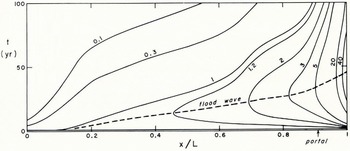
Fig. 3b. The same as Figure 3a but showing lines of equal 1 on an x : t diagram. The broken line shows the progress of the flood wave. Numbers against curves are the values of h1 in meters
We have not used the influence coefficients explicitly in assessing the future behaviour of the glacier in the neighbourhood of the tunnel portal for the following reason. The future behaviour is the sum of (1) the response to past mean mass balances and (2) the response to future mean mass balances. The past mean mass balances of the glacier have not been measured, and in the present state of knowledge it is impossible to infer them from measurements on other glaciers. (We refer here to the time variation of the mean mass balance over the glacier surface, rather than the x variation of the mass balance. It is possible to infer the latter from other glaciers, but not the former.) Nevertheless the relevant information on past mean mass balances is actually present in the glacier in the form of a distribution of h 1(x), and if h 1(x) were known (which it is not), the future response to past mean mass balances could, in principle, be worked out completely. This response to past mass balances would of course include the present retreat rate as one of its features. Component (2) of the future behaviour depends on the future climate. If limits are set to the possible future mass balances, limits may correspondingly be fixed for the glacier response, and the most convenient way of doing this is by use of the e(n) coefficients. However, in the present application the only information we have on (1) is the present retreat rate, and it is therefore better to use the polynomial method, with the λ coefficients, that we have described.
The influence coefficients g(n) follow a pattern similar to that previously found for South Cascade Glacier and Storglaciären.
The frequency response at x = 7 990 is shown in Figure 4. The curves are similar to those in Reference NyeNye (1965[a]). The curve of phase lag against frequency shows a single maximum at a period of 52 years.

Fig. 4. Computed frequency response at x = 7 990 m (x/L = 0.91) to a periodic variation in mean mass balance of unit amplitude. The amplitude |H| and phase lag ϕ of the response are plotted against the angular frequency ω


