


l. Introduction
Basal ice temperature plays an important role in controlling ice velocity and consequently, ice-sheet geometry and discharge. If basal ice is at the pressure melting point, basal water is generated which can enhance the sliding velocity. At temperatures lower than the melting point, ice temperature affects ice stiffness and deformational velocity. Therefore, estimating the basal temperature of ice sheets is critical for generating realistic results using numerical ice-sheet models. Our current knowledge about spatial variations of basal temperature, however, is poorly constrained by observations and in situ measurements that only present the local basal temperatures.
The amount of heat generated at the base of an ice sheet governs the basal ice temperature. This heat can derive from three major sources: heat generated from the internal deformation of ice, heat produced from the friction of ice with the glacier bed, and geothermal heat flux from the Earth's interior (GHF). The effect of each of these components on basal conditions varies spatially, primarily based on ice thickness, velocity and tectonic setting. Among these sources, GHF has the largest uncertainty range in the interior regions; apart from a handful of deep ice cores, direct measurements of GHF are not available under the ice sheet.
The importance of spatial variations in GHF on ice-sheet dynamics has been discussed in several studies (e.g. Larour and others, Reference Larour, Morlighem, Seroussi, Schiermeier and Rignot2012; Rogozhina and others, Reference Rogozhina2012; Pittard and others, Reference Pittard, Galton-Fenzi, Roberts and Watson2016). Modeling studies show that GHF not only affects the basal thermodynamic condition but also alters the thickness and surface geometry of ice sheets (Greve and Hutter, Reference Greve and Hutter1995; Larour and others, Reference Larour, Morlighem, Seroussi, Schiermeier and Rignot2012). Therefore, understanding the spatial distribution of GHF is important for enhancing the robustness of ice-sheet models.
At ice core locations, GHF can be inferred from the measured vertical temperature gradient in the basal ice layer and the thermal conductivity of ice. Measurements from ice cores reveal large variations in GHF over short distances (tens of kilometers) in the Greenland Ice Sheet (GrIS). For example, the estimated GHF from the NGRIP ice core (~140 mW m−2, Dahl-Jensen and others, Reference Dahl-Jensen, Gundestrup, Gogineni and Miller2003) is more than 50% higher than GHF measurements at the GRIP ice core, located roughly 300 km away (51.3 mW m−2, Dahl-Jensen and others, Reference Dahl-Jensen1998). In addition, GHF estimates at the onset of the Northeast Greenland Ice Stream (NEGIS) may be an order of magnitude higher than at the GRIP ice core, only 200 km away (Fahnestock and others, Reference Fahnestock, Abdalati, Joughin, Brozena and Gogineni2001). In south Greenland, at the location of the Dye-3 ice core, the modeled GHF suggests low values of roughly 20 mW m−2 (Gundestrup and Hansen, Reference Gundestrup and Hansen1984; Greve, Reference Greve2005). Among the six deep ice cores shown in Greenland, only two of them contain evidence of basal thaw: NGRIP (Dahl-Jensen and others, Reference Dahl-Jensen, Gundestrup, Gogineni and Miller2003) and NEEM (Goossens and others, Reference Goossens2016) (Fig. 1). Although spatial variations in GHF are shown to have significant effects on the thermodynamics of basal ice, they remain a large unknown in Greenland.
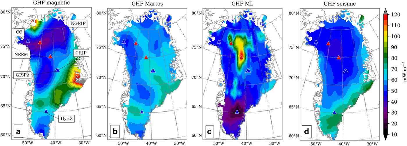
Fig. 1. The GHF maps that are used in this study from (a) Fox Maule and others (Reference Fox Maule, Purucker and Olsen2009), (b) Martos and others (Reference Martos2018), (c) Rezvanbehbahani and others (Reference Rezvanbehbahani, Stearns, Kadivar, Walker and van der Veen2017) (ML refers to machine learning) and (d) Shapiro and Ritzwoller (Reference Shapiro and Ritzwoller2004). The fifth GHF map is spatially uniform GHF of 56 mW m−2. Ice cores sites are shown with triangles with blue and red colors indicating observed frozen and thawed basal conditions, respectively. The Camp Century ice core is denoted by CC.
Direct measurements of GHF of the GrIS are limited to a few deep ice core sites. To overcome this limitation, several methods have been developed to predict the spatial patterns of GHF. For example, Fox Maule and others (Reference Fox Maule, Purucker and Olsen2009) use remotely-sensed magnetic data to calculate the Curie depth, from which the GHF can be inferred (Fig. 1a). The analysis of magnetic data is advanced by Martos and others (Reference Martos2018) who use spectral analysis to estimate the depth of Curie isotherm in Greenland from high-resolution magnetic anomaly data (Fig. 1b). Rezvanbehbahani and others (Reference Rezvanbehbahani, Stearns, Kadivar, Walker and van der Veen2017) train a machine learning algorithm by combining the global GHF measurements and geologic and tectonic properties to predict the GHF in Greenland (Fig. 1c). In addition, seismic tomography models, based on structural similarity functionals, are used to estimate the global GHF (Shapiro and Ritzwoller, Reference Shapiro and Ritzwoller2004) (Fig. 1d), and Greve (Reference Greve2005) and Greve (Reference Greve2019) modify the empirical GHF estimates of Pollack and others (Reference Pollack, Hurter and Johnson1993) to match the modeled and measured basal temperatures in Greenland ice cores.
Seismic and magnetically-derived maps of Shapiro and Ritzwoller (Reference Shapiro and Ritzwoller2004) and Fox Maule and others (Reference Fox Maule, Purucker and Olsen2009) have been used in thermo-mechanical ice-sheet models to estimate the basal temperature of the GrIS (e.g. Rogozhina and others, Reference Rogozhina2012; Seroussi and others, Reference Seroussi2013); however, the calculated basal temperatures often do not match deep ice core measurements. Using spatially uniform GHF values in numerical ice-sheet models may yield more accurate results for surface elevation reconstructions and temperature profiles at ice core sites than other GHF models (e.g. Rogozhina and others, Reference Rogozhina2012). Consequently, applying a spatially uniform GHF for GrIS is still common in modeling studies.
Radar surveys are pivotal in identifying regions with temperate bed or ponded water. Basal water or temperate bed is not explicitly a boundary condition in modeling ice-sheet behavior. However, the existence of basal temperate ice sets an important constraint on the thermal boundary condition of the bed; it implies that the GHF must be larger than a critical value below which the bed would be frozen (referred to as GHFpmp). Therefore, numerical ice-sheet models can implement the spatial distribution of radar-detected basal water to estimate GHFpmp. Such results are necessary to evaluate the reliability of current GHF models.
This study seeks to improve our understanding of basal thermal conditions of the GrIS by constraining the spatial variations of GHF according to the extent of thawed basal state, predicted by radar data. It also aims at demonstrating and highlighting the contrasts between GHF models and GHF constraints obtained from radar data. We use two datasets that independently predict the location of basal melt of the GrIS. The first dataset is from Oswald and others (Reference Oswald, Rezvanbehbahani and Stearns2018) where they use the acuity of the reflected radar signals (Oswald and Gogineni, Reference Oswald and Gogineni2008, Reference Oswald and Gogineni2012) to delineate regions where subglacial water likely exists. This dataset identifies thawed regions with substantial basal water thickness (~3 cm, Oswald and others, Reference Oswald, Rezvanbehbahani and Stearns2018). The second dataset is from Jordan and others (Reference Jordan2018), who use a ‘bed-echo reflectivity variability’ method, based on the reflection intensity of the radar signals, to detect wet–dry transitions in the basal material. Both datasets are purely based on radar data and are independent of numerical or GHF models. Note that in both datasets, not detecting temperate ice or ponded water at the bed does not imply that the bed is frozen. In other words, the implemented criteria to determine the basal condition is a necessary condition, but not sufficient.
Here we use the three-dimensional thermo-mechanical ice-sheet model SICOPOLIS (Greve and Hutter, Reference Greve and Hutter1995; Greve, Reference Greve1997) to iteratively estimate the GHF at locations where basal water is detected. By adjusting the value of GHF at thawed points, we constrain the GHF of the ice sheet so that the basal condition matches the predictions of both of these radar studies. We then compare the GHFpmp values with the available GHF maps in Greenland, namely, seismically derived (Shapiro and Ritzwoller, Reference Shapiro and Ritzwoller2004), magnetically derived (Fox Maule and others, Reference Fox Maule, Purucker and Olsen2009), machine learning-based (Rezvanbehbahani and others, Reference Rezvanbehbahani, Stearns, Kadivar, Walker and van der Veen2017, referred to as ML) and the GHF from spectral analysis of high-resolution magnetic data (Martos and others, Reference Martos2018).
A similar approach has been conducted by Van Liefferinge and Pattyn (Reference Van Liefferinge and Pattyn2013) and Van Liefferinge and others (Reference Van Liefferinge2018) in order to identify the possible locations with a frozen bed in East Antarctica in search for the oldest ice. Since the regions that are investigated in those studies are in the interior regions of East Antarctica, vertical one-dimensional models would suffice. However, because some of the regions of interest in our study are near the margins, the effect of horizontal heat advection and thermo-mechanical coupling becomes important (e.g. Rezvanbehbahani and others, Reference Rezvanbehbahani, van der Veen and Stearns2019b) and a three-dimensional model is necessary.
The structure of this study is as follows: we first introduce the thermal component of the numerical ice-sheet model, SICOPOLIS and simulation set up (Section 2.1). Then, we explain the two radar datasets of Oswald and others (Reference Oswald, Rezvanbehbahani and Stearns2018) and Jordan and others (Reference Jordan2018) that are used in this study (Section 2.2). We present the results of adjusting the GHF at the locations of radar-detected basal water (Section 3.1), perform sensitivity analysis with respect to different climatic conditions (Section 3.2), and compare the estimated constraints against the GHF models (Section 3.3). We discuss the uncertainty of the estimates, as well as an in-depth comparison with ice core data that reveal several discrepancies between different datasets. Then we investigate several mechanisms that can resolve these discrepancies and finally investigate the importance of such constraints on the total melt-water production at the base of the ice sheet (Section 4).
2. Data and methodology
2.1. Ice-sheet model and simulation set-up
We use the SImulation COde for POLythermal Ice Sheets (SICOPOLIS version 3.3) to iteratively solve for GHF. SICOPOLIS simulates the dynamic and thermodynamic evolution of ice sheets using the Shallow Ice Approximation (SIA, Hutter, Reference Hutter1983). Glacier ice is treated as a heat-conducting incompressible fluid with power-law rheology (Glen, Reference Glen1955), regularized to avoid infinite viscosities in the limit of small effective stresses (Greve and Blatter, Reference Greve and Blatter2009). Given a time-dependent external forcing (climate conditions), SICOPOLIS simulates the temporal evolution of ice thickness, temperature and velocity field.
We model the thermal evolution of GrIS using the enthalpy method (e.g. Aschwanden and others, Reference Aschwanden, Bueler, Khroulev and Blatter2012). This method has the advantage of including temperature and water content in a single thermodynamic variable. Specifically, in order to simulate the thermal evolution of the ice sheet, we use the one-layer melting-CTS enthalpy scheme of SICOPOLIS, which explicitly enforces the transition conditions at the CTS (continuity of the temperature gradient and water content) for any polythermal ice column (Blatter and Greve, Reference Blatter and Greve2015; Greve and Blatter, Reference Greve and Blatter2016).
At the surface of the ice sheet, atmospheric temperature is applied as a constant Dirichlet-type boundary condition, and at the base, GHF is included as a constant Neumann-type heat flux. A Weertman-type sliding law is implemented everywhere at the base. At regions with a frozen bed, sub-melt sliding is introduced following Hindmarsh and Le Meur (Reference Hindmarsh and Le Meur2001) to avoid singularity in the calculation of the velocity field at the transition between frozen and thawed bed regions. Frictional heating is included in the thermal boundary condition as the product of sliding velocity and basal shear stress (which in the case of SIA equals the driving stress).
We use a spatial resolution of 20 km which leads to a grid of 140 × 82 points in the stereographic plane. Sigma coordinates are used in the vertical direction (z): each ice column is mapped onto a [0, 1] interval, discretized by 81 vertical grid points. For modeling the thermal conduction in the underlying bedrock, we use 41 layers in the thermal lithosphere. The creep enhancement factor is chosen as a constant value of 1 for Holocene ice (<11 ka) and 3 for Pleistocene ice (>11 ka) (similar to Greve, Reference Greve2005; Rogozhina and others, Reference Rogozhina2012). The rest of the physical parameters are the same as those of Rückamp and others (Reference Rückamp, Greve and Humbert2019, Table 1). Since the simulations are not in steady-state condition, a model for the glacial isostatic adjustment must be included to simulate the changes in bed elevation due to changes in the ice load. We use the Local-Lithosphere-Relaxing-Asthenosphere model (LLRA) with a time lag of 3000 years for relaxing the asthenosphere (following Le Meur and Huybrechts, Reference Le Meur and Huybrechts1996).
Input parameters to the model include average annual and monthly surface temperatures, annual surface mass balance, global sea level and GHF. Paleoclimate temperature variations across the ice sheet are modeled by implementing a time-dependent temperature anomaly function ΔT(t), such that


where T ma and T mj represent present-day's mean annual and July temperatures (from Fausto and others, Reference Fausto, Ahlstrøm, Van As, Bøggild and Johnsen2009); ϕ and λ denote latitude and longitude, respectively, and S is the surface elevation of the ice sheet. Temperature anomaly function is reconstructed using δ18O records from the NorthGRIP ice core since the last interglacial at −120 ka until −4 ka (Andersen and others, Reference Andersen2004). The time series is extended to the previous glacial maximum at ~−140 ka by ΔT linearly decreasing to − 20°C. From −4 ka to present, the reconstruction by Kobashi and others (Reference Kobashi2011) derived for the GISP2 site is used. The climate anomaly function is shown in Figure 2 and is spatially uniform.
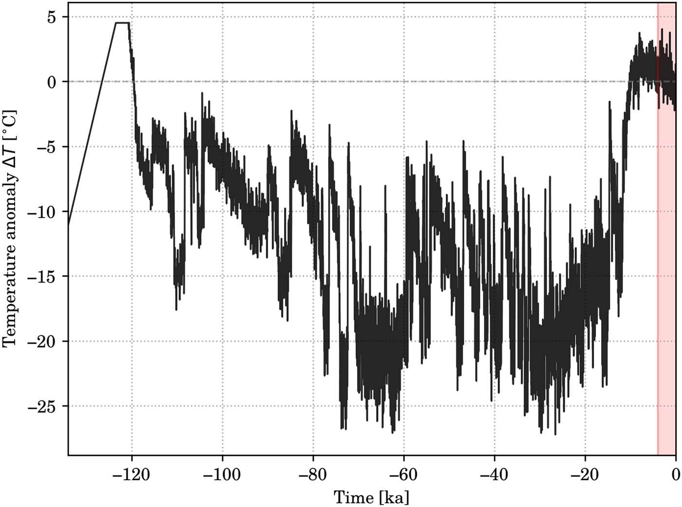
Fig. 2. Time series for the temperature anomaly (ΔT) used in Eqn (1). The last 4 ka (light-red shading) are reconstructed from Kobashi and others (Reference Kobashi2011) while the rest of the anomaly is from the NorthGRIP ice core δ18O record (Andersen and others, Reference Andersen2004).
We use monthly mean for present-day precipitation for the 1958–2001 period, obtained from the regional energy and moisture balance REMBO by Robinson and others (Reference Robinson, Calov and Ganopolski2010), provided with a spatial resolution of 100 km. Following Huybrechts (Reference Huybrechts2002), at every time step we assume 7.3% change in precipitation for a 1°C surface temperature change. Solid precipitation is calculated monthly using an empirical 5th order polynomial (Bales and others, Reference Bales2009). We have used the positive degree day (PDD) parameterization from Reeh (Reference Reeh1991) for estimating the surface melt with a semi-analytical solution for the PDD integral obtained by Calov and Greve (Reference Calov and Greve2005). For ice melt, the PDD factor βice = 8 mm w.eq. d−1 °C−1 is used, while for snow melt βsnow = 3 mm w.eq. d−1 °C−1. For global sea level history, we use the reconstruction from the SPECMAP marine δ18O records provided by Imbrie and others (Reference Imbrie, Berger, Imbrie, Hays, Kukla and Saltzman1984).
In numerical ice-sheet models, GHF is applied as a boundary condition to the thermal model, which itself is strongly tied to the mechanical model. Therefore, inversion for GHF in thermo-mechanically coupled ice-sheet models is very challenging. Studies have attempted to formulate and solve the inverse problem for GHF (e.g. Zhu and others, Reference Zhu2016). However, their analysis is limited to a cold ice sheet with a no-slip basal condition. This assumption makes their method unsuitable for the current study, because frictional heating is an important heat source especially near the margins of the ice sheet. Therefore, we apply an iterative scheme that incrementally adjusts the GHF in a forward model.
In this study, we start the paleoclimate simulations at − 134 ka and all simulations are composed of three steps:
(1) First, the present-day geometry of GrIS provided by Bamber and others (Reference Bamber2013) is relaxed for 100 years to create a smoothed geometry of the ice sheet.
(2) From −134 to −9 ka, the ice sheet freely evolves given the initial and boundary conditions. The starting time of −134 ka is chosen because at that time ΔT = −11.3°C, which is close to the mean temperature anomaly over the entire period. Basal sliding is gradually ramped up during the first 5 ka of this step. This transitional period is required to avoid numerical stability problems, while being short enough not to influence the further evolution of the ice sheet significantly.
(3) From −9 ka to the present, the results of step (2) are used as initial conditions, and the computed ice-sheet topography (surface S(x, y), bed b(x, y)) is continuously nudged toward the slightly smoothed present-day topography (surface S target(x, y), bed b target(x, y)) produced by step (1). Starting the nudging process at −9 ka allows the ice sheet to evolve freely during the last glacial and the transition into the Holocene, thus preserving the paleo-climatic memory. For each time step, this nudging is done by first solving the normal evolution equations for the bed and the ice thickness (e.g. Greve and Blatter, Reference Greve and Blatter2009, Eqns (5.55) and (8.5)) and then applying the relaxation equations
(3)$$\displaystyle{{\partial S} \over {\partial t}}{\rm } = -\displaystyle{{S-S_{{\rm target}}} \over {\tau _{{\rm relax}}}},$$ (4)$$\matrix{ {\displaystyle{{\partial b} \over {\partial t}}} \hfill & { = -\displaystyle{{b-b_{{\rm target}}} \over {\tau _{{\rm relax}}}},}}$$with a relaxation time of τrelax = 100 a (Rückamp and others, Reference Rückamp, Greve and Humbert2019). This is equivalent to applying an SMB correction (e.g. Calov and others, Reference Calov2018), which is diagnosed by the model.

Because the goal is to estimate the GHF required to reach the bed to the pressure melting temperature, at the end of step (3) we check the basal thermal conditions at the locations of radar-detected basal thaw: if T b (relative to the pressure melting point) is colder than − 0.1°C, we increase the GHF by 5%. Otherwise, if the basal melt rate $\dot M_{\rm b}$ at these locations is larger than 0.001 m a−1, we decrease the GHF by 5%. We terminate the simulations after 50 iterations of steps (1) through (3) when the majority of regions of interest have met the pressure melting point's criteria. Note that throughout the iterative procedure, we assume that basal water is due to basal melting at the same location (and not generated in other places and transported to that region), nor does it derive from surface or englacial water that has reached the bed (e.g. Poinar and others, Reference Poinar2015, Reference Poinar2017).
Since SICOPOLIS is thermo-mechanically coupled, the thermal properties at the locations where GHF is not adjusted impacts the flow field, and hence they impact the thermal properties of all regions. Therefore, we estimate GHFpmp for both radar detections of basal thaw, using five independent simulations with different initial GHF models; four simulations are with the GHF models shown in Figure 1, and one simulation with a spatially uniform GHF of 56 mW m−2 (denoted by U56, corresponding to the average GHF value of the North American plate, Sclater and others, Reference Sclater, Jaupart and Galson1980).
2.2. Datasets for radar-detected basal thaw
The spatial distribution of the basal thermal state is determined from two sources. The first dataset from Oswald and others (Reference Oswald, Rezvanbehbahani and Stearns2018, hereafter OSW) is essentially based on the character of reflected radar signals from the ice-bed interface (after Oswald and Gogineni, Reference Oswald and Gogineni2008, Reference Oswald and Gogineni2012). Basal state determinations based on radar data (provided by Center for Remote Sensing of Ice Sheets, CReSIS during 1999–2003; Gogineni and others, Reference Gogineni2001) are made approximately every 200 m along each radar flight line; melt detections are separated along the flight path by one ice thickness and the conditions for melting are assumed to be effectively continuous between melt detections. Circles are then drawn on the effectively continuous melting path segments, and an assumption of isotropy of the basal state distribution is used to infer the probable state across the flight path. This means that determinations from neighboring flight paths can be used in support of interpolated basal states and the effect of random detection errors is minimized. If two adjacent paths contradict each other, the priority is given to the non-ponded determinations. This technique allows for larger scale interpolation of the basal state of the ice, as opposed to narrow radar flight paths. The detected basal water using this method represents ‘ponded’ basal water that is thicker than ~3 cm. The rest of the regions could be frozen or temperate with a thinner layer of basal water. The spatial distribution of basal ‘ponded water’ from Oswald and others (Reference Oswald, Rezvanbehbahani and Stearns2018) is shown in Figure 3a.

Fig. 3. Spatial distribution of radar-detected basal water from (a) Oswald and others (Reference Oswald, Rezvanbehbahani and Stearns2018)-OSW, and (b) Jordan and others (Reference Jordan2018)-JOR. The datasets provided by the two studies are grouped in 100 km polygons and then sampled at 20 km spacing to represent the spatial resolution of SICOPOLIS that is used in this study.
The second dataset is from Jordan and others (Reference Jordan2018, hereafter JOR) who develop a new diagnostic method for inferring basal thermal state from radio echo sounding data. Their method, termed ‘bed-echo reflectivity variability’, uses bed-echo intensity and acts as an edge-detector to identify the locations where rapid transition between wet–dry bed occurs. Jordan and others (Reference Jordan2018) show that their method is not affected by spatial variability in attenuation and can be adjusted to be used with different radar systems employed in different Operation IceBridge surveys. They interpret their results as ‘basal water distribution’ and every pick corresponds to a circle with 5 km diameter as the effective resolution of their method (see Jordan and others, Reference Jordan2018, Fig. 6). The spatial distribution of basal water from Jordan and others (Reference Jordan2018) is shown in Figure 3b.
In order to implement the scattered radar points from the two datasets into a 20 km SICOPOLIS grid, we create polygons using individual radar picks from both studies (with an aggregate distance of 100 km). Then, every SICOPOLIS grid point that falls within the created polygons are chosen as the targeted thawed points in SICOPOLIS. The aggregate distance of 100 km for creating the polygons is chosen after several experiments with different aggregate distances. This distance results in the best spatial representation of both radar datasets. Admittedly, this method over-interprets the locations of basal water, since not all the radar points in a 20 km pixel are necessarily inferred to be thawed using radar data. The uncertainties associated with such interpretation are discussed in Section 4.
The focus of this study is to set constraints on GHF based on the spatial distribution of thawed beds predicted by these two studies. Assessing the causes of the observed differences between the two datasets is beyond the scope and aim of the current work. However, it is worth mentioning that in both of these datasets, not detecting a thawed bed or ponded water does not indicate that the bed is frozen. Therefore, their differences are not necessarily contradictions; they rather show the strength or weakness of one of the radar techniques compared to the other.
3. Results
We calculate GHFpmp at the locations of basal thaw predicted by OSW and JOR separately. For each of these datasets, we perform five different simulations with all the GHF models considered in this study: at the locations where GHF is not being adjusted (referred to as ‘background’ GHF), the GHF values remain fixed as prescribed by each GHF model. Here we present the mean and standard deviation (STD) of all the GHF constraint estimates for both radar datasets (see Figs S1 and S2 for details of individual simulations with different background GHF values).
If the calculated GHF constraints are high, it is reasonable to ask whether frictional heating is responsible instead of a high GHF. In the majority of points where GHF is adjusted, a frozen bed is switched to a thawed bed during the iterative process. This switching has resulted in an increase in both surface and basal sliding velocities compared with the initial state. This means that a previously frozen bed has become thawed after GHF adjustments, and even though the frictional heating is now added to the basal heat budget, the GHF constraint is still increased. Therefore, at the radar-points where GHF is adjusted, if the final basal velocity is increased (and consequently augmented the basal frictional heating) after GHF adjustments, our presented GHF constraints remain valid and our arguments hold.
On the other hand, it is possible that the final velocity after adjusting the GHF results in a lower surface and basal sliding velocity. This is more likely near the margins of the ice sheet where the interaction between fast flowing and slow moving ice becomes more complex. Interpreting the calculated GHF constraints becomes more challenging in such locations, because the portion of the adjusted GHF to reach the bed could have been due to the lowering of frictional heating. Frictional heating is a function of basal shear stress and sliding velocity, therefore, we investigated the regions where either of these two variables has decreased after the iterations (which has resulted in reduced frictional heating). Since this source of heat can be substantial in finding the GHF constraints, we remove the points with G friction-init − G friction-final < −5 mW m−2 for all simulations (5 mW m−2 subjectively assumed as a reasonable ‘margin of error’ for GHFpmp estimates). This ensures that the GHF constraints presented in the study are not ‘contaminated’ by the effect of decrease in frictional heating. Note that the offsets between the final modeled vs. present-day geometry are not sufficient to make a notable difference on changes in strain heating.
3.1. GHFpmp at thawed points
Figure 4 shows the estimated GHFpmp values, averaged for all five simulations at thawed-bed predictions by OSW (Fig. 4a) and JOR (Fig. 4c) (corresponding standard deviations, STD, shown in Figs 4b, d). Regardless of the ‘background’ GHF, the GHFpmp estimates are consistent for the majority of thawed regions.

Fig. 4. Average and standard deviation (STD) of GHFpmp at basal thaw detections by OSW (a,b) and JOR (c,d). For GHFpmp values using individual GHF background maps, see Supplementary Figs S1 and S2.
For thawed points in the central-east region of OSW data, southeast of the GISP2 and GRIP ice cores, the average GHFpmp is between 70 and 90 mW m−2 (Fig. 4a). Near the NGRIP ice core site, our estimates show that GHF of ~70 mW m−2 is sufficient to thaw the bed. Slightly downstream of the NGRIP site toward the northeast region, GHFpmp is smaller with values near 40–50 mW m−2. In the northwest region close to the Camp Century (CC) ice core site, despite the extent of basal thaw being rather small, the GHFpmp is relatively high with values greater than 85 mW m−2 (Fig. 4a).
Because of the greater spatial extent of JOR dataset, the GHF constraints using this dataset contain more spatially detailed information. The GHF constraints in the northern parts of interior regions close to the NGRIP ice core site are within the range of 55–75 mW m−2 (Fig. 4c). In contrast, the estimated GHFpmp decreases downstream of NGRIP toward the northeast region of the ice sheet and upstream of the 79North glacier to values as low as 10 mW m−2. These regions, despite having such low GHFpmp values still experience basal melt rates higher than our cut-off criterion (i.e. $\dot M_{\rm b}<0.001$ m a−1). The low GHFpmp values in the entire western flank of the ice sheet are similar to those of the downstream reaches of the northeast Greenland. Apart from a few scattered points, the low GHFpmp persists in the entire low-elevation regions in western Greenland.
In contrast to the low GHFpmp regions, two regions stand out for having a notably high GHFpmp values using the JOR dataset. In central-east and northern parts of the GrIS, GHFpmp values as high as 100–120 mW m−2 are estimated (Fig. 4c). At several of these points, the cut-off criterion for basal temperature relative to the pressure melting point (i.e. T b > −0.1°C) was not achieved and the simulation was terminated after 50 iterations (see Section 2.1).
3.2. Simplified sensitivity analysis
The results presented here contain paleoclimate simulations that are enforced based on climate reconstructions of ice cores and marine δ18O records. Therefore, they carry uncertainties that can alter the present results. Given the computational expense of the iterative simulations presented here, performing sensitivity analysis on climatic parameters is extremely costly. Therefore, we analyze the sensitivity of GHFpmp estimates at several anomalous locations with a 1D analytical solution of the temperature profile of ice sheets. We use the solution provided by Rezvanbehbahani and others (Reference Rezvanbehbahani, van der Veen and Stearns2019b) which is an improvement to the Robin (Reference Robin1955) analytical solution and allows estimating the GHFpmp given the surface temperature, ice thickness and surface mass-balance rate. Although the solution is obtained in steady-state conditions (unlike the SICOPOLIS simulations presented here), it facilitates analyzing the sensitivity of GHF constraints on a wider range of climatic variables. We assess the sensitivity of high GHFpmp estimates near CC, Dye-3 and central-east regions of the GrIS.
The CC and Dye-3 ice cores are near ice divides and the horizontal velocities are small. Therefore, the conditions are suitable to use a 1D analytical solution for the vertical temperature near this site. Thickness of the CC and Dye-3 ice cores is ~1400 and 2000 m, respectively. In the central-east region of the ice sheet where the GHFpmp estimates from SICOPOLIS are high, thickness values range from a few hundred to ~1000 m. Because the analytical solution is in steady-state, we use a range of input variables for surface mass-balance rate and surface temperature to calculate the GHFpmp.
During the 1960–1990 period (during which net accumulation matched the net ablation, Van den Broeke and others, Reference Van den Broeke2009), the surface mass balance from regions obtained from RACMO2/GR (Ettema and others, Reference Ettema2010) ranges between ~0.4 and 0.8 m a−1 ice equivalent with surface temperatures ~−30 to −20°C for all the three regions of interest. We use a wider range of surface mass-balance rate values (0.1–1 m a−1), as well as surface temperatures ranging from − 40 to − 10°C.
The GHFpmp calculations from the 1D analytical solution are shown in Figure 5; Figures 5a, b represent the central-east regions; Figures 5c, d correspond to CC and Dye-3 ice core regions, respectively. This simple sensitivity analysis confirms that the central-east region requires a significantly higher GHF to thaw the bed. It also shows that at the CC ice core site, where RACMO2/GR reports surface temperature of −25°C and surface mass-balance rate of ~0.4 m a−1, the GHF value of roughly 90 mW m−2 is needed to thaw the bed (Fig. 5c). The value of GHFpmp is ~60 mW m−2 for Dye-3 with surface mass-balance rate of ~0.65 m a−1 and surface temperature of −19°C. Considering that both these ice cores have measured basal temperatures ~−13°C, the actual GHF is likely much less than GHFpmp estimates in this section.

Fig. 5. GHFpmp calculated from the 1D analytical solution provided by Rezvanbehbahani and others (Reference Rezvanbehbahani, van der Veen and Stearns2019b). The GHFpmp is calculated for four thickness values of (a) 500 m, (b) 1000 m, (c) 1400 m and (d) 2000 m and a range of surface temperature values T s from − 10 to − 40°C. The x-axis represents the surface mass balance, $\dot M$ . The thickness ranges of (a) and (b) are chosen to represent the central-east region of the GrIS, while (c) is chosen to represent the CC ice core, and (d) represents the Dye-3 ice core.
3.3. Comparing GHFpmp vs. GHF models
The GHF constraints calculated here are the lower limits of GHF to produce basal thaw, so the GHF models must be larger than the constraints if they are to properly simulate the detections of basal thaw. Figure 6 shows the spatial differences between GHFpmp and GHF models at locations of basal thaw for both radar datasets, and Figure 7 is a scatter representation of such differences. Because the uncertainties in all GHF models are relatively high, the ‘acceptable’ range for GHF models is chosen such that GHF − GHFpmp ≥ −5 mW m−2. The percentage values indicated on each map in Figure 6 shows the ratio of the points in each GHF map that are acceptable with respect to the estimated GHF constraints.

Fig. 6. Comparing the GHFpmp estimates at thawed points of OSW (a–e) and JOR (f–j) with respect to different GHF maps. The percentage values in each panel shows the ratio of points in each GHF map that are ‘acceptable’ according to the estimates constraints defined as (#of points with GHF − GHFpmp ≥ −5 mW m−2)/#total points.
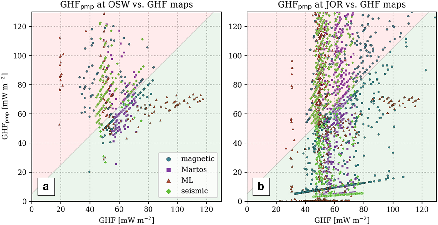
Fig. 7. Difference between the GHF maps (x-axis) and calculated GHF constraints (y-axis). The green region is where GHF − GHFpmp ≥ −5 mW m−2, as the ‘acceptable’ difference with respect to the calculated constraints.
There are several locations where the GHF models satisfy their lowest constraint imposed by GHFpmp. The most notable of all are the downstream regions of almost the entire western margin of the ice sheet where JOR dataset predicts extensive basal thaw. Our estimated GHF constraints are very small and all GHF models satisfy the constraints. Other notable regions are the northeast of the NGRIP ice core (from OSW dataset) and approximate location of the downstream of NEGIS upstream of 79North glacier (from JOR dataset).
In contrast, however, several regions from both datasets result in very high GHF constraints that are not satisfied in any of the GHF models. The most prominent one is the central-east region at 30°W, 70°N and to the north at ~30°W, 73°N. The values from GHF models in this region are substantially smaller than the required heat flux to thaw the bed. Other regions of disagreement are around the CC ice core (from both radar datasets), scattered points near Dye-3 (Figs 6a–e), and the northern margin of the ice sheet (Figs 6f–j).
4. Discussion
4.1. GHF constraints and ice core data
There are regions of basal thaw in the central-east catchment of the ice sheet where the GHFpmp values are estimated to be very high. There are no deep ice cores in this area to confirm or reject such high GHF estimates. Nearly all GHF models predict elevated GHF values in the eastern edge of Greenland (at 70°N, 30°W, Fig. 1), but except for the magnetically-derived GHF map of Fox Maule and others (Reference Fox Maule, Purucker and Olsen2009), none of the maps predict GHF values as high as 100 mW m−2. Although several of the current GHF models predict a high heat flux in the eastern regions (along the trajectory of Icelandic plume), only the GHF reconstruction of Rogozhina and others (Reference Rogozhina2016) and more recently Artemieva (Reference Artemieva2019) predict GHF values as high as 100 mW m−2 in east Greenland. This region is suggested to have lower lithosphere viscosity as well as a higher temperature compared to the rest of the cratonic settings in Greenland (Mordret, Reference Mordret2018). Therefore, the extensive basal thaw in the central-east region may be associated with GHF variations due to the remnant of the Icelandic plume.
The basal temperature at the GISP2 and GRIP ice core sites are reportedly cold at ~−9°C (Dahl-Jensen and others, Reference Dahl-Jensen1998). Both radar datasets detect water a few tens of kilometers to the east of these ice cores. The GHF to match the basal temperature measurements at the GRIP ice core site is 51 mW m−2 (Greve, Reference Greve2019). The value of GHFpmp at the basal thaw determinations in these regions is estimated to be close to the continental average (~70 mW m−2). Given that the distance between GRIP/GISP2 ice core sites and the closest cluster of basal water determinations from the two datasets is ~30–40 km, we suggest that the observed basal thaw in this region can be associated to spatial variations in the GHF.
Radar determinations of basal thaw or ponded water near Dye-3 and CC ice core sites are rather surprising. The basal temperatures at Dye-3 and CC ice cores are both near −13°C (Dansgaard and others, Reference Dansgaard, Johnsen, Møller and Langway1969; Gundestrup and Hansen, Reference Gundestrup and Hansen1984), far below the pressure melting temperature. The matching GHF to reproduce these basal temperatures in SICOPOLIS are 32 mW m−2 for Dye-3 and 47 mW m−2 for CC (Greve, Reference Greve2019). Our results show that GHFpmp ranges between 70 and 90 mW m−2 near Dye-3 and is over 100 mW m−2 near the CC ice core site (Fig. 4). Comparison between the GHF models and estimated GHFpmp shows that neither of the GHF models predict such high GHF values in these regions (see Section 3.3). The closest cluster of basal thaw determinations from Jordan and others (Reference Jordan2018) dataset is ~5 km away from the CC ice core and the closest cluster of ponded water from Oswald and others (Reference Oswald, Rezvanbehbahani and Stearns2018) is more than 10 km away. While there is no standard expected length-scale for spatial variations in GHF, it is unlikely that GHF can vary so drastically in such small spatial scales (<10 km). The contrast between the GHF at ice cores and GHFpmp in close vicinity of the core sites indicates that the basal thermal conditions could vary over much shorter spatial scales than commonly assumed.
4.2. Possible mechanisms for local GHF variations
The apparent contradiction between detection of basal thaw from radar data and very low basal temperatures from ice cores cannot be reconciled without considering other local mechanisms that can alter the local heat flux at the bed. The first mechanism is suggested by Van der Veen and others (Reference Van der Veen, Leftwich, Von Frese, Csatho and Li2007) who show that variations in topography (such as troughs and valleys) alter the local GHF so that topographic lows experience enhanced heat fluxes at edges, while the topographic highs have lower heat flux peaks. Given the rough nature of subglacial topography (especially in the central-east regions, Rippin, Reference Rippin2013; Rezvanbehbahani and others, Reference Rezvanbehbahani, van der Veen and Stearns2019a), it is possible that such high GHF fluctuations do actually occur at such small spatial scales (<10 km).
The second possible explanation is hydrothermal circulation that can augment the basal heat flux due to the interaction of subglacial groundwater and basal ice. The modeling study by Gooch and others (Reference Gooch, Young and Blankenship2016) suggests that during the retreat phase of ice sheets, the vertical water discharge from sedimentary aquifers in the subglacial environment can add to the net heat budget at the base of the ice sheet. In Greenland, geophysical surveys have identified regions of saturated till at the bed (e.g. Christianson and others, Reference Christianson2014); but the study of subglacial aquifers has gained little attention. These two mechanisms, however, occur at a much smaller spatial scale than the GHF models presented here. Therefore, special attention should be dedicated to small-scale processes that can result in significant and short-scale variations of GHF.
The third mechanism to elevate the GHF is due to the ‘vug-wave’ fluid migration processes (PhippsMorgan and Holtzman, Reference PhippsMorgan and Holtzman2005); due to the loading and unloading during the glacial and inter-glacial phases, Stevens and others (Reference Stevens, Parizek and Alley2016) show that molten magma at depth can migrate through faults and dyke emplacement which can substantially augment the basal heat flux. This mechanism is hypothesized to alter the Greenland's heat flux on a substantially larger scale and impact the overall stability of the GrIS (Alley and others, Reference Alley2019).
Our results indicate that the lower elevation regions of western Greenland, even with low GHF values of 10 mW m−2, undergo substantial basal thaw (Figs 4 and 6f–j). This indicates that there is a very high certainty that these regions are almost entirely temperate. However, the analysis of radar data does not show a continuous determination of basal water (see Jordan and others, Reference Jordan2018, Fig. 6; Oswald and others, Reference Oswald, Rezvanbehbahani and Stearns2018, Fig. 11). Our findings demonstrate that the extent of basal thaw in these regions is significantly larger than what is inferred from radar data. This confirms Jordan and others (Reference Jordan2018)'s note that their criterion for basal thaw is necessary but insufficient (and that their results only show ‘rapid spatial transitions’ in basal condition). Similarly, it is possible that rapid drainage of the basal water or the shallow depth of basal water prevents ponded water detections by Oswald and others (Reference Oswald, Rezvanbehbahani and Stearns2018) method. We suggest that this region can serve as a proper location for improving the analysis of radar data, because according to the analysis presented here, it is likely extensively thawed at the bed.
4.3. Catchment-wide $\dot M_{{\rm b}}$ estimates

The GHF models for Greenland analyzed in this study bear almost no resemblance to each other (Fig. 1). Without direct borehole measurements and some indirect geologic and glaciologic proxies (e.g. the onset location of the Northeast Greenland Ice Stream, NEGIS, or the possible trajectory of the Icelandic plume), there is no straightforward way to confirm or reject the current models. These GHF models undoubtedly lead to different spatial distributions of basal thaw in Greenland (e.g. Rogozhina and others, Reference Rogozhina2012). It is crucial, however, to investigate whether these different models and their ‘modified’ versions (which include the GHFpmp estimates in this study) result in substantial differences in terms of the amount of basal water generated in Greenland.
In order to evaluate the impact of GHF differences and the calculated constraints on the net basal melt rate in Greenland, we calculate the annual rate of basal melt-water produced in each catchment of Greenland with a) all five GHF maps (as in Fig. 1 and U56), (b) modified GHF models in Figure 1 by setting the GHF values to GHFpmp at the regions of disagreement (Section 3.3) according to OSW dataset, and (c) same as case (b) but modified according to the distribution of JOR dataset. In other words, the ‘modified’ GHF maps are GHFmod = max (GHF, GHFpmp).
Comparison between the values of total basal melt rate shows that although the spatial distribution of temperate bed may vary substantially depending on the GHF model, the total magnitude of basal melt-water remains relatively unchanged (Table S1). The net basal melt rate of GrIS using different GHF models is ~15–20 km3 a−1, substantially smaller than the range of surface mass loss in Greenland (Fettweis and others, Reference Fettweis2013; Csathó and others, Reference Csathó2014). However, it has important implications for estimating the continuous year-round discharge from the base of outlet glaciers. It is worth noting that since we have not included a subglacial hydrology model (e.g. de Fleurian and others, Reference de Fleurian2018; Sommers and others, Reference Sommers, Rajaram and Morlighem2018), our estimates do not take into account the interactions between subglacial hydrological network and GHF. Such interactions can alter the ice velocity and may consequently change the basal thermal regime of the ice sheet. This may be a topic for future studies.
4.4. Modeling shortcomings and radar uncertainties
Throughout the iterative procedures in all the simulations of this study, the aim has been to keep the GrIS geometry intact. Because the iterations using Oswald and others (Reference Oswald, Rezvanbehbahani and Stearns2018) dataset involved fewer points, the geometry and surface velocity has been reconstructed relatively well (Fig. S1). However, the spatial extent of the basal thaw based on Jordan and others (Reference Jordan2018) is much larger. Therefore, the substantial adjustments to the GHF have resulted in altering the geometry of the ice sheet; these alterations are more notable toward the margins and insignificant in the interior regions (Fig. S2). Due to thermo-mechanical coupling of the ice flow, local enhancement of GHF changes the flow and geometry, specifically in the low-velocity regions (Pittard and others, Reference Pittard, Galton-Fenzi, Roberts and Watson2016). Changes in the velocity profile of the ice sheet alter the rate of advection from upstream, therefore altering the thermal field of the neighboring points. Therefore, it is not surprising that the GHFpmp based on either OSW or JOR datasets varies depending on the initial choice of GHF map.
The effective resolution of JOR dataset is ~5 km, and the internal consistency method of OSW results are provided in 1 km spatial scale. Due to the high computational cost of performing the iterative procedure in 5–10 km spatial resolution, we clustered the locations of basal thaw from the two datasets into 20 km spatial resolution. This clustering is an exaggeration of the extent of thaw for both basal water datasets. The determinations of temperate basal ice from the radar data could be associated to enhanced localized heat flux (e.g. Van der Veen and others, Reference Van der Veen, Leftwich, Von Frese, Csatho and Li2007) or a complex distribution of subglacial water (e.g. Schroeder and others, Reference Schroeder, Blankenship and Young2013; Chu and others, Reference Chu, Schroeder, Seroussi, Creyts and Bell2018; Bowling and others, Reference Bowling, Livingstone, Sole and Chu2019). In order to reconstruct such small-scale details of basal heat and direction of subglacial water flow, higher resolution models coupled with a dynamic hydrologic component must be considered (e.g. Dow and others, Reference Dow2018).
In all the presented results, we have neglected the uncertainties in thaw determinations from radar data. Analyses of the radar bed-echo characteristics are not unique; it is possible that the thaw interpretations can actually be due to variations in basal roughness, or a combination of basal thaw and roughness variations. Therefore, additional research must be conducted to enable the differentiation of basal roughness variations and regions of basal thaw from radar data.
5. Conclusion
We use the locations of basal water in Greenland, detected by two radar datasets to constrain the GHF in Greenland using SICOPOLIS numerical model. The GHF at these locations is iteratively adjusted so that the basal temperature or basal melt rates become near zero, hence finding the minimum GHF that is required to reach the bed to the pressure melting point (GHFpmp). We conduct the iterative simulations with different initial GHF models of Greenland to resolve the uncertainty associated with the initial basal thermal condition on the final constraints. Although there are locations whose GHF constraints differ depending on the initial GHF model, there are persistent regions where the constraints are anomalously high or low. The most prominent regions with anomalously low GHFpmp values include a large part of the low-elevation regions of the western flank of the ice sheet, as well as in the northeast region, downstream of NEGIS.
We find several regions with GHFpmp values as high as 100 mW m−2. The largest region with high GHFpmp is in the central-east of the ice sheet, to the east of GISP2 and GRIP ice cores; in all simulations the estimated GHFpmp is ~100–120 mW m−2. Our results also highlight sharp contrasts between low basal temperature readings from CC and Dye-3 ice cores and prediction of basal water by both radar datasets. We argue that the existence of water in close proximity to these ice cores cannot be explained by the spatial variability of GHF; we posit that such sharp contrasts can be better explained by the effect of elevated heat flux near the topographic edges (Van der Veen and others, Reference Van der Veen, Leftwich, Von Frese, Csatho and Li2007), the interplay between glacial loading and volcanism in the underlying crust (Stevens and others, Reference Stevens, Parizek and Alley2016; Alley and others, Reference Alley2019), or the discharge of groundwater aquifers into the subglacial environment and elevating the basal heat flux (Gooch and others, Reference Gooch, Young and Blankenship2016). These mechanisms are not currently incorporated in GHF or glaciologic models and can help resolve the current discrepancies between modeled and observed basal thermal state of the GrIS. Finally, we show that despite all these differences in GHF maps and uncertainties in reconciling observations with our model, the net basal melt-water production does not significantly differ depending on the GHF model.
Supplementary material
To view supplementary material for this article, please visit https://doi.org/10.1017/jog.2019.79
Acknowledgments
We thank Thomas Jordan for providing the data for basal thaw detection, Michiel van den Broeke for the RACMO2 dataset and Gunter Leguy for insightful discussions. We also thank scientific editor Frank Pattyn and two anonymous reviewers for their constructive comments that greatly improved the clarity of this manuscript. S.R. was supported by the NSF grant ANT0424589, L.A.S. was supported by the NASA grant NNX10AP05G and C.J.V. was supported by the NSF grant ARC0909422. G.K.A.O. acknowledges NSF ARRA Grant 0909431, by the University of Maine Climate Change Institute. R.G. was supported by the Japan Society for the Promotion of Science (JSPS) through KAKENHI grant numbers JP16H02224 and JP17H06104, and by the Japanese Ministry of Education, Culture, Sports, Science and Technology (MEXT) through the Arctic Challenge for Sustainability (ArCS) project.


 Open access