

Introduction
Melt layers in ice sheets form during exceptionally warm conditions. Records of melt layers in ice cores can therefore give insight into changes in summertime peak temperatures, recording the frequency of extremely warm summers (Reference Herron, Herron and LangwayHerron and others, 1981; Reference Langway and ShojiLangway and Shoji, 1990; Reference Alley and AnandakrishnanAlley and Anandakrishnan, 1995; Reference Kameda, Narita, Shoji, Nishio, Fujii and WanatabeKameda and others, 1995; Reference Das and AlleyDas and Alley, 2008).
Melt also significantly decreases the albedo of the snow surface, which triggers a positive feedback. As a result, it is useful to understand the history of surface melting in order to successfully model the radiative balance of an ice sheet (e.g. Reference Tedesco, Serreze and FettweisTedesco and others, 2008, Reference Tedesco2011; Reference Box, Fettweis, Stroeve, Tedesco, Hall and SteffenBox and others, 2012). In addition, the study of recent melt events is important for estimating the mass balance of the ice sheet, because refrozen meltwater is not lost from the ice sheet, and affects firn density and thus mass-balance estimates from repeated altimetry (e.g. Reference Pfeffer, Illangasekare and MeierPfeffer and others, 1990, Reference Pfeffer, Meier and Illangasekare1991; Reference Harper, Humphrey, Pfeffer, Brown and FettweisHarper and others, 2012; Reference ForsterForster and others, 2014; Reference Morris, Mair, Nienow, Bell, Burgess and WrightMorris and others, 2014). The observed correlation of melt layers between different ice-core sites shows that melt layers often arise from widespread meteorological events, and can reflect regional climate conditions (Reference Kameda, Narita, Shoji, Nishio, Fujii and WanatabeKameda and others, 1995; Reference Das and AlleyDas and Alley, 2008). Satellite imaging of recent melt events that extended over much of Greenland (Reference Tedesco, Serreze and FettweisTedesco and others, 2008; Reference NghiemNghiem and others, 2012; Reference Hall, Comiso, DiGirolamo, Shuman, Box and KoenigHall and others, 2013; Reference McGrath, Colgan, Bayou, Muto and SteffenMcGrath and others, 2013) supports this view.
When the surface or near-surface snow melts, the liquid water percolates down into the firn and spreads along thin, near-surface crusts, subsequently refreezing into a melt layer when the air temperature lowers, or incoming radiation drops (Reference Langway and ShojiLangway and Shoji, 1990; Reference Pfeffer and HumphreyPfeffer and Humphrey, 1998; Reference Das and AlleyDas and Alley, 2005; Reference Wong, Hawley, Lutz and OsterbergWong and others, 2013). Melt layers appear in bubbly ice cores as near-horizontal, typically irregular or discontinuous bands of ice with few, oddly shaped or sized, air bubbles, typically 1–100 mm thick (Fig. 1; Reference Langway and ShojiLangway and Shoji, 1990; Reference Das and AlleyDas and Alley, 2005). The visual identification of melt layers can be complicated by another type of bubble-free feature: thin crusts, usually a single grain in thickness ( 1 mm), which are observed in all seasons (Reference Fujii and KusunokiFujii and Kusunoki, 1982; Reference Alley and AnandakrishnanAlley and Anandakrishnan, 1995). The origin of these crusts is poorly understood, and they probably have multiple origins (Reference AlleyAlley, 1988), including glazing by wind action (Reference Albert, Shuman, Courville, Bauer, Fahnestock and ScambosAlbert and others, 2004), vapor transfer (Reference Fujii and KusunokiFujii and Kusunoki, 1982) or even some slight melting (Reference Alley and AnandakrishnanAlley and Anandakrishnan, 1995). Prior interpretations of melt features generally have been restricted to thicker, nearly bubble-free layers, which include other indications of melt, such as large grains, anomalously large, elongated bubbles, and lenticular shape (Reference Langway and ShojiLangway and Shoji, 1990; Reference Alley and AnandakrishnanAlley and Anandakrishnan, 1995; Reference Das and AlleyDas and Alley, 2005).

Fig. 1. Melt layers from the NEEM (North Greenland) ice core at 44.3 m. This melt event is dated to AD 1888. Photo courtesy of Kaitlin Keegan.
As we explore further back in time using deeper ice, melt layers are harder to identify due to thinning of the layers with depth and air clathrate formation. Air clathrates form when the pressure is sufficient to change the air bubble within the ice into a solid phase, in which the air is surrounded by water molecules, forming a lattice (Reference MillerMiller, 1969).
At sufficiently great depth, typically below 1250 m (Reference FitzpatrickFitzpatrick and others, 2014), the air bubbles have completely changed to air clathrates, thus precluding visual identification of melt layers. As a result, a chemical identification of melt layers is essential to study melt events during warm periods beyond the Holocene, for instance the last interglacial (NEEM community members, 2013).
Melt layers have a strong influence on the gas composition of the ice core: soluble gases (e.g. carbon dioxide, methane, nitrous oxide, krypton and xenon) can dissolve in the liquid water before it freezes, and induce very high concentrations of these gases in the ice core (Reference Ahn, Headly, Wahlen, Brook, Mayewski and TaylorAhn and others, 2008; NEEM community members, 2013). While CH4 and N2O are clearly elevated in melt layers, these gases may also be produced by microbes in ice, so they cannot serve as reliable indicators of refrozen meltwater (NEEM community members, 2013).
We present here a method to use noble gases as a reliable test of the presence of refrozen meltwater in ice-core samples, and describe two applications: testing for the presence of melt events during the Eemian at the NEEM (North Greenland Eemian Ice Drilling) ice-core site, and analyzing the composition of the pervasive bubble-free layers present in the West Antarctic Ice Sheet (WAIS) Divide ice-core site.
Melt-Layer Detection using Krypton and Xenon in Ice Cores
Krypton and xenon are highly soluble in liquid water, and both are more soluble than argon. Therefore, Kr/Ar and Xe/ Ar ratios are higher in melted and refrozen ice than within air bubbles in ice that has not melted. We show that these noble gas ratios may be used as additional, independent indicators of melt layers in ice cores.
Theory
Fractionation due to melt
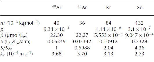
Xenon is approximately four times, and krypton two times as soluble as argon (Table 1; Reference Wood and CaputiWood and Caputi, 1966; Reference WeissWeiss, 1970; Reference Weiss and KyserWeiss and Kyser, 1978). As a result, Kr/Ar and Xe/Ar ratios are higher in melted and refrozen ice than within air bubbles in ice that has not melted, and exhibit a specific relationship.
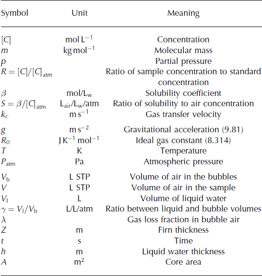
Table 1. Parameter values. Solubility coefficients (β) are calculated at 0°C (Reference Weiss and KyserWeiss and Kyser, 1978; Reference Hamme and EmersonHamme and Emerson, 2004). Gas transfer velocities (kc ) are from Reference Nicholson, Emerson, Caillon, Jouzel and HammeNicholson and others (2010) and Reference Cole, Bade, Bastviken, Pace and Van de BogertCole and others (2010), with Schmidt numbers from Reference Jähne, Heinz and DietrichJähne and others (1987). p, β, S and kc are given for the bulk Kr and Xe rather than for a specific isotope
The solubility equilibrium is expressed in terms of the solubility coefficient β, expressed in mol L−1 of liquid water:
We report the ratios (R) in delta notation, δ = (R/R standard − 1) 1000, and use modern atmospheric air as our standard. In order to compare the meltwater ratio to the atmospheric ratio, we define S Ar = β Ar/[Ar]atm, the solubility in liters of air per atmosphere per liters of liquid, with [Ar]atm being the concentration of argon in the atmosphere (mol L−1 atm−1).
The solubility ratios of Xe and Kr with Ar are therefore


We can also express these as δ(Xe/Armelt) = (4.36 − 1) 1000 = 3360 ‰, and similarly, δ(Kr/Armelt) = 1004‰.
Therefore, it appears that not only are samples containing refrozen melt enriched in Kr/Ar and Xe/Ar in comparison to non-melted ice, but a pure melt end-member will also show a unique relationship between δ(Kr/Ar) and δ(Xe/Ar), with a slope of ∼3.3.
The refreezing process contributes to the exclusion of atoms and molecules whose size is larger than that of the crystal spacing of the ice, which includes Ar, Kr and Xe (Reference Top, Martin and BeckerTop and others, 1988). Experiments done on the growth of frazil ice (Reference Top, Martin and BeckerTop and others, 1988) and on the freezing of lake water show that 1–50% of the noble gases are retained, likely depending on the freezing rate, and that there is no clear indication of fractionation of Kr/Ar or Xe/Ar during refreezing (Reference Malone, Castro, Hall, Doran, Kenig and McKayMalone and others, 2010).
Gravitational fractionation
In non-melted ice, measured Kr/Ar and Xe/Ar are primarily affected by gravitational fractionation (Reference Craig and WiensCraig and Wiens, 1996). Gravitational fractionation is a process in which heavier isotopes are preferentially concentrated with increasing depth in firn. According to Reference Craig, Horibe and SowersCraig and others (1988), gravitational fractionation is described by the barometric equation modified for a gas pair:

where δgrav is the gravitational fractionation of an isotope pair, g is the local gravitational acceleration, Z is the thickness of the firn, Δm is the mass difference between the two isotopes, R 0 is the gas constant and T (K) is the temperature of the firn column. The mass difference Δm = 96 for δ(Xe/Ar), and it is Δm = 48 for δ(Kr/Ar). As a result, we expect a δ(Xe/Ar) vs δ(Kr/Ar) slope of 2 in gas samples from non-melted ice.
Gas loss
Kr/Ar and Xe/Ar ratios can also be affected by gas loss during air bubble close-off and during core storage. Gas loss affects molecules with a diameter smaller than 3.6 Å (3.6 × 10⁻¹⁰ m), including Ar and O2 but not N2, Kr and Xe (Reference Bender, Sowers and LipenkovBender and others, 1995; Reference Severinghaus and BattleSeveringhaus and Battle, 2006). As a result, gas loss will cause Kr/Ar and Xe/Ar to be slightly higher than expected. In order to remove the effects of gas loss, we can compute δ(Xe/Kr), which is independent of Ar:
We expect that for meltwater, δ(Xe/Kr) ≈ 1177‰. A sample with refrozen melt will have elevated δ(Xe/Kr).
Analysis of Kr/Ar and Xe/Ar in known melt layers
The ice-core samples analyzed in the first part of this study were from the Holocene, taken from the Dye 3 ice core. Dye 3 is a site in South Greenland (65° N, 43° W; 2480 m a.s.l.), with a mean annual temperature of −21°C and an annual accumulation rate of 0.49 m a−1 (Reference Dahl-Jensen and JohnsenDahl-Jensen and Johnsen, 1986). The core contains numerous visible melt layers, identified as horizontal bands of ice with few air bubbles, a few mm to a few cm thick (Reference Langway and ShojiLangway and Shoji, 1990). We analyzed samples containing melt layers at 144 m. We also sampled ice that did not contain visible melt layers at 143–145 m depth, and refer to it as non-melted ice. The ice-core Kr/Ar and Xe/Ar are measured following the technique outlined by Reference Severinghaus, Grachev, Luz and CaillonSeveringhaus and others (2003) and Reference Headly and SeveringhausHeadly and Severinghaus (2007). Ice samples are typically 50–60 g each, measured in duplicate or triplicate for a given depth. The standard used in these measurements is air collected from the Scripps pier in La Jolla, CA, USA. The method used to collect the air is described in Reference Headly and SeveringhausHeadly and Severinghaus (2007).
The δ(Kr/Ar) and δ(Xe/Ar) measured in Holocene ice from the Dye 3 ice core are shown in Table 2 and Figure 2. The data show different trends in melted versus non-melted ice. The δ(Kr/Ar) and δ(Xe/Ar) in melt layers are clearly enriched compared with those of non-melted ice. The melt-layer values range from 30‰ to 63‰ for δ(Kr/Ar), and 69‰ to 168‰ for δ(Xe/Ar). Non-melted ice samples from Dye 3, in contrast, have δ(Kr/Ar) values of 13.0 ± 2.0‰, and δ(Xe/Ar) of 24.5 ± 3.8‰. There are large variations of δ(Kr/Ar) and δ(Xe/Ar) for replicate samples of melt layers from the same depth, which shows that δ(Kr/Ar) and δ(Xe/Ar) are not quantitative indicators of melt intensity, or that the fraction of refrozen meltwater varies strongly over short distances (Table 2).
Table 2. Measurements of the Dye 3 ice core. Samples with visible melt layers are shown in bold font (144.2–144.31 m and 144.47–144.6 m). Replicates from the same depth are labeled a, b, c, etc. The air content (column 4) is expressed as the ratio of the sample with respect to the mean of all non-melt samples. The rightmost three columns show the calculated diffusive column height Z, the gas loss fraction λ and the melt fraction γ. The mean and standard deviation of all non-melt samples give an idea of the expected sample-to-sample variability. The pooled standard deviation σ pooled describes the measurement error
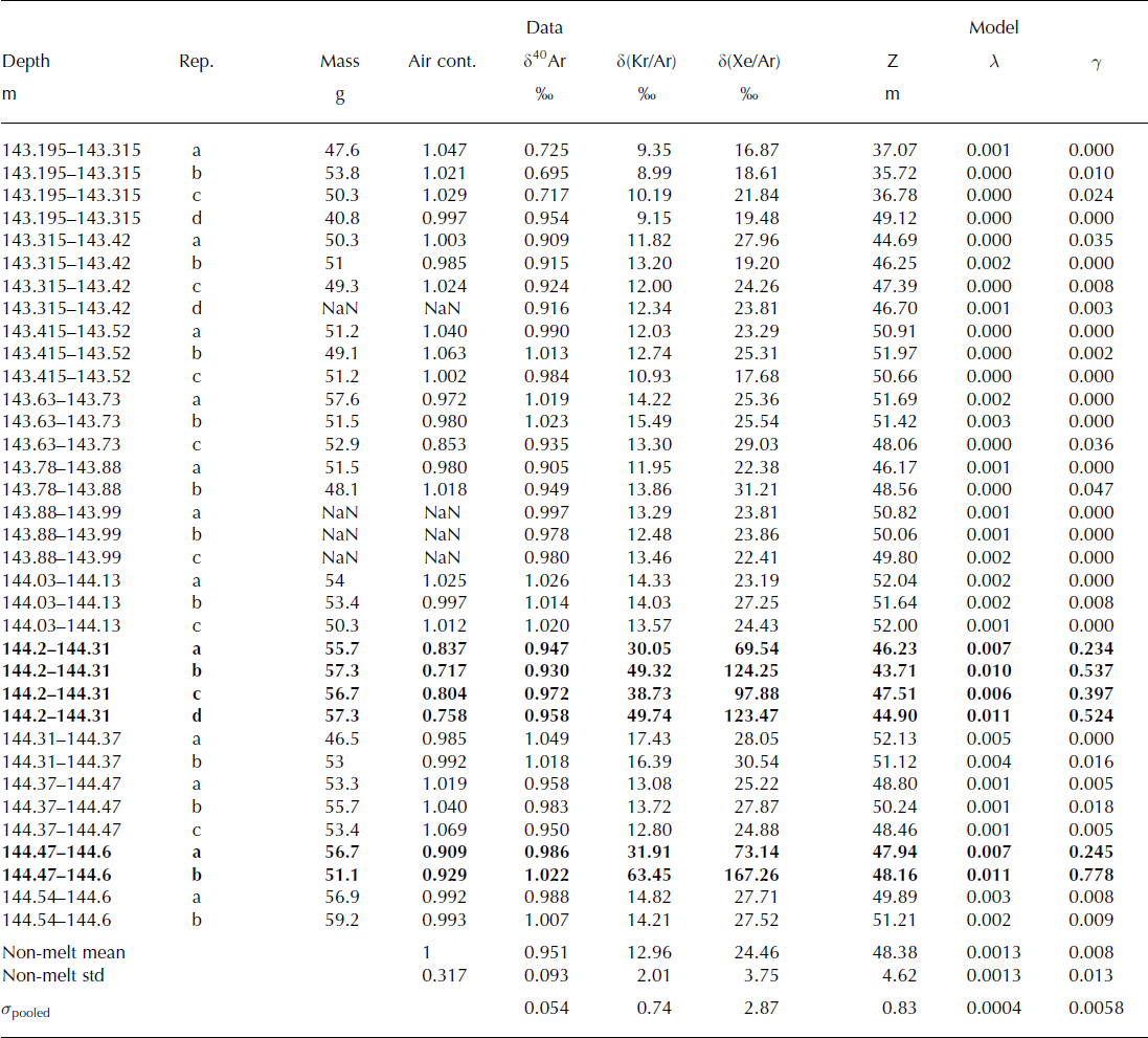

Fig. 2. Melt layer identification. When δ(Kr/Ar) and δ(Xe/Ar) are high, they indicate the presence of melt, as can be seen in Dye 3 melt layer samples (solid diamonds), compared to non-melt samples (+). NEEM Eemian samples are shown in large squares. The analytical precision is better than 0.8‰ for δ(Kr/Ar) and 2.9‰ for δ(Xe/Ar), which is approximately the size of the markers. WAIS Divide bubble-free layers (filled circles) do not have anomalously high δ(Kr/Ar) and δ(Xe/Ar), which indicates that they do not contain a significant amount of melt. The box shows the range of values found in the WDC05A ice core. The dashed line indicates gravitational fractionation, and the solid lines indicate the fractionation due to melt.
We also find that the slope of δ(Xe/Ar) vs δ(Kr/Ar) is 3.01, which is in agreement with that predicted from theory for gases at solubility equilibrium, and confirms that the possible expulsion of gases during refreezing does not alter the melt signature in the ice. The slope of δ(Xe/Ar) vs δ(Kr/Ar) for non-melt samples is 1.77, which is slightly lower than the expected slope (2) due to gravitational fractionation, possibly due to an incomplete degassing of Xe in the sample.
Quantification of the amount of melt
A typical ice-core sample contains both air from bubbles (called Arair in the following) and from dissolved gas (called Armelt). In order to quantify the amount of refrozen water in a sample, we model the respective contributions of (1) gravitational fractionation, (2) melt and (3) gas loss as follows (units are moles of gas):
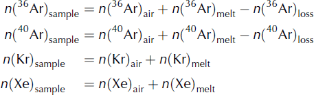
The ‘air’ terms (e.g. n(Ar)air) in Eqns (6) represent the abundance of each gas in the air bubble within the ice core. The abundance in the air bubbles reflects both the atmospheric abundance at the time the air was trapped (e.g. Aratm), as well as the effects of gravitational fractionation on the gases in the firn. The concentration of argon in the air bubbles [Ar]air is related to the atmospheric concentration [Ar]atm as
If we denote V b the volume of the air bubbles, the number of moles of argon in the air bubbles is n(Arair) = V b[Ar]air.
The ‘melt’ terms reflect the enrichment of these gases due to the presence of melt layers. Argon, krypton and xenon are partially expelled during freezing; thus, a portion of the refrozen melt will be gas-free, and will not contribute to anomalies in ice-core gas composition. We quantify the volume of refrozen water that retained the melt signature V l and find that the quantity of dissolved gas follows
The 36Arloss term represents Ar loss due to gas loss from the ice core. Gas loss typically causes δ40 Ar/36 Ar in the air that remains in an air bubble to be positively enriched by 0.007‰ per 1‰ δ(Kr/Ar) enrichment (Reference Severinghaus, Grachev, Luz and CaillonSeveringhaus and others, 2003). Therefore, 40Ar is slightly less depleted by gas loss than 36Ar: n(40Ar)loss = 0.993(n(36Ar)loss). We denote λ as the fraction of gas lost, so we can write
We use atmospheric air as our standard gas. If we denote V the total volume of gas in the sample, the number of moles of argon in the reference gas is n(Arstandard) = V[Ar]atm. This implies that the ratio of sample to standard is

We note γ = V l/V b the ratio of the volume of liquid water to the volume of gas in the bubbles. The equation becomes
Following the same pattern for the other observed gases, we can rewrite the system of Eqn (6) in terms of our observations (δ40 Ar/36 Ar, δKr/Ar and δXe/Ar) and the three parameters

To solve the system of equations above, we calculate Z, γ and λ by iterated linearized inversion. The results from six different melt-layer samples from shallow ice from the Dye 3 ice core are shown in Table 2. The calculated firn depth Z and gas loss λ are consistent in all replicates, but the wide range of values for γ, the volume ratio of refrozen meltwater to bubble air, shows that the extent of melt is not a spatially uniform parameter in an ice-core sample.
Melt Events during the Last Interglacial at Neem
The last interglacial, the Eemian (130–115 ka BP), was warmer than the current interglacial in many places including Greenland, owing to higher insolation forcing (Reference Francis, Wolfe, Walker and MillerFrancis and others, 2006; Reference Otto-BliesnerOtto-Bliesner, 2006; Reference Axford, Briner, Francis, Miller, Walker and WolfeAxford and others, 2011; Reference Masson-DelmotteMasson-Delmotte and others, 2011; Reference LuntLunt and others, 2012). A recent study at the NEEM site in North Greenland (77.45° N, 51.06° W; 2450 m a.s.l.; −29°C) shows that the temperature may have been 8 ± 4°C warmer than present at constant elevation (NEEM community members, 2013). The analysis of CH4 and N2O in NEEM ice shows brief intervals of very high concentrations: up to 2000 ppb in CH4 for a background of ∼750 ppb, and up to 400 ppb in N2O for a background of 250 ppb. However, these values are higher than can be explained by solubility alone, and point towards a significant contribution of in situ production of CH4 and N2O by microbes present in the ice (NEEM community members, 2013).
We measured δ40 Ar, δ(Kr/Ar) and δ(Xe/Ar) in NEEM samples from the Eemian, between 2398 and 2403 m, and found δ(Kr/Ar) values between 17.73‰ and 56.47‰, and δ(Xe/Ar) values between 22.60‰ and 166.94‰ (Fig. 3). In order to save precious ice, we used 30 g, 3.5 cm samples, and diluted them 20 times with pure N2. The rest of the analytical method is the same as for Dye 3 samples (Reference Severinghaus, Grachev, Luz and CaillonSeveringhaus and others, 2003). We calculated the melt fraction (γ) of all samples, and found that 21 out of 39 samples had γ > 0.1, corresponding to at least 1% of the mass of the sample being refrozen water (1 mL of air is typically found in a 10 g ice-core sample). These measurements confirm the presence of melt layers in the interval 127–118.3 ka BP.

Fig. 3. Measurements of δ40 Ar, δ(Kr/Ar) and δ(Xe/Ar) in the Eemian section of the NEEM ice core. The dashed line on top shows the modeled melt fraction, inferred from the measurements. Elevated δ(Kr/Ar) and δ(Xe/Ar) are clear evidence of the presence of melt in the ice core.
Very few melt layers have been observed at the NEEM ice-coring site above the clathrate transition, although the extreme heatwave of 12–15 July 2012 produced melt at NEEM, as well as on >98.6% of the Greenland ice sheet (Reference NghiemNghiem and others, 2012; Reference McGrath, Colgan, Bayou, Muto and SteffenMcGrath and others, 2013). Contrary to the Dye 3 samples (65° N, 44° W; −21°C), which contained melt from a single event, the NEEM Eemian samples each cover about a decade. Yet the melt fractions are comparable, with three samples above γ = 0.5. This suggests that the magnitude and/or frequency of Eemian melt events was larger than in the Holocene at Dye 3, which is consistent with up to 8 ± 4°C higher temperature, and high summer insolation (NEEM community members, 2013).
The presence of melt layers at NEEM during the Eemian confirms that the additional warmth had a strong summer component, which is consistent with the fact that the eccentricity was much higher during the last interglacial than during the Holocene, enhancing the impact of precession and seasonal contrasts at that time.
Analysis of Bubble-Free Layers in the WAIS Divide Ice Core
The WAIS Divide ice core provides the highest-resolution gas record of the last 60 000 years (e.g. Reference MarcottMarcott and others, 2014). The WAIS Divide site is located in Antarctica (79° S, 112° W; −29°C, 0.22 m ice a−1), where dust fluxes are minimal, and in situ production of greenhouse gases is much smaller than in Greenland. It is also in a high-accumulation region, which allows for a small gas-age–ice-age difference (∼500 years at the Last Glacial Maximum (Reference BuizertBuizert and others, 2014)), and a small uncertainty in the gas chronology, including during Termination 1, unlike existing East Antarctic deep ice cores such as Dome C or Vostok.
Upon physical inspection of the core, we noticed a very large number of bubble-free layers, ∼1–2 mm thick (Fig. 4), at a rate of ∼15 (m (ice))−1, or 4a−1. They are visible in layers deposited during all seasons, with a higher occurrence in the late summer, as measured using the position relative to the summer peak of the annual-layer counted timescale (WAIS Divide Project Members, 2013; Fegyveresi, 590 2014). They can only be detected in the first 600 m of the core: the bubbles disappear in the deeper part of the core, due to the formation of air hydrates under high hydrostatic pressure, making the ice clear, and the bubble-free layers visibly indistinguishable from the rest of the ice (Reference FitzpatrickFitzpatrick and others, 2014).

Fig. 4. A pair of bubble-free layers in the WDC05A core. The layers are 1 mm thick. Black in this image represents clear ice, and bubbles appear white. Photo by John Fegyveresi.
Similar bubble-free layers have been documented in other ice cores (Reference Fujii and KusunokiFujii and Kusunoki, 1982; Reference AlleyAlley, 1988; Reference Alley and AnandakrishnanAlley and Anandakrishnan, 1995) and have been interpreted as the remnants of surface crusts, which can be several mm thick, but typically much thinner. These crusts can have multiple origins, and current understanding includes the possibility that some crusts may contain refrozen meltwater.
It is important for the accuracy of the gas record to know whether these layers contain sufficient melt to compromise the soluble gas record, and whether they affected gas diffusion through the firn, thereby complicating the gas chronology.
Influence on gas composition
To test for the presence of significant melt, we analyzed two samples containing bubble-free layers, and three control samples, taken between 114 and 147 m in the WDC05A ice core, which was collected at the site the year before the main deep core (Reference AhnAhn and others, 2012). All of these samples were taken from mature ice, well below the bubble-closure depth, which is at ∼78 m at WAIS Divide (Reference BattleBattle and others, 2011). Each sample was prepared using a bandsaw to cut across the core, extracting a slab ∼5 mm thick containing the 1 mm crust. Several slabs were pooled into one 600 g sample. Control samples consisted of the same number of slabs of bubbly ice, taken from neighboring ice (Table 3). The samples were melted under vacuum to release the trapped air. The air sample was then exposed to a Zr/Al getter at 900°C to remove N2, O2 and other reactive gases, and the resulting gas was expanded into a MAT 252 mass spectrometer to measure δ40 Ar, δ86/82 Kr, δ(Kr/Ar), δ(Xe/Ar) and δ(Ne/Ar) (Reference OrsiOrsi, 2013).
Table 3. Analysis of bubble-free layers in the WDC05A ice core. The δ values are given in ‰ with respect to modern air. Z, λ and γ are the outputs of the melt layer model. The bottom two rows show the mean and standard deviation of 73 WDC05A samples measured from 38 depths between 78 and 300 m. The uncertainty in the modeled Z, λ and γ and is calculated by a Monte Carlo perturbation with variances corresponding to the bottom row of the table, and is also shown in the bottom row
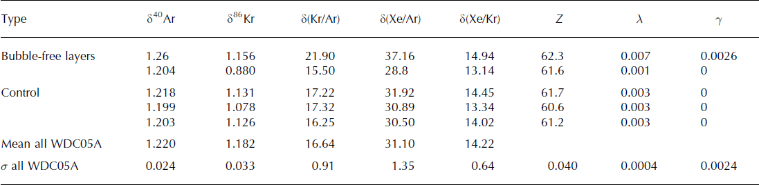
The first bubble-free sample is slightly elevated in Kr and Xe: when compared to the standard deviation of all ice-core measurements taken together (noted σ all), δ(Kr/Ar) is 5.4σ all higher than the control samples, and δ(Xe/Ar) is 4.5σ all all higher than the control samples (Table 3). However, we have used very thin samples, which can be subject to the loss of argon through cut bubbles and permeation (Reference Severinghaus and BattleSeveringhaus and Battle, 2006). We calculated the respective contributions of gravitational fractionation, gas loss and melt for all samples (Table 3), and found more gas loss than other samples (λ = 0.007 ± 0.0004), and a melt contribution that is not statistically significant (γ = 0.0026 ± 0.0024).
We thus conclude that the 1 mm bubble-free layers in the WAIS Divide ice core are unlikely to contain any significant amount of melt, and do not alter the gas composition of the ice core. This observation is confirmed by the studies of CO2 in the same WDC05A core, which show no sensitivity to the presence of a bubble-free layer in a sample (Reference Ahn, Brook and HowellAhn and others, 2009). The absence of melt is also supported by the observation that the bubble-free layers occur in winter as well as in summer (Reference FegyveresiFegyveresi, 2014). A possible mechanism for the formation of a bubble-free layer is the infilling of pores by condensation on a surface crust during times of subsurface temperature inversion (Reference Fujii and KusunokiFujii and Kusunoki, 1982). This is consistent with the prevalence of these layers in late summer, when the surface is cooler than the firn (Reference FegyveresiFegyveresi, 2014), and suggests that we may be able to use the frequency and thickness of bubble-free layers as a proxy for the occurrence of surface temperature inversions. The formation of these layers could also involve other mechanisms and is the subject of another paper (Reference FegyveresiFegyveresi, 2014).
Influence on gas diffusion
Gases diffuse through the firn before getting locked in within a zone in which the air is separated from the atmosphere, at ∼66 m depth at WAIS Divide (Reference BattleBattle and others, 2011). The firn matrix determines the effective gas diffusivity, which impacts the width of the age distribution of bubble air, and the lock-in horizon, which determines the age difference between gases and ice, and ultimately the gas chronology. The presence of an impermeable layer can thus sharpen the gas age distribution by preventing diffusion, and create an abrupt change in the gas chronology.
When they are in the firn, bubble-free layers are likely to have lower permeability than the surrounding firn. We were actually unable to find ice lenses in 2 m snow pits dug in 2008, 2009 or 2010, but we found evidence for numerous hard ‘crusts’ (Fig. 5c). In addition, these crusts typically have a limited spatial extent, on the order of 3 m × 10 m, and they can be broken by what looks like thermal-contraction cracks, through which gases can flow (Fig. 5b).

Fig. 5. Hard surfaces (‘crusts’) seen at WAIS Divide (a). These crusts are hard enough that the weight of a person does not puncture through. They can be laced by cracks, likely formed by thermal contraction (b). The thickness of these crusts can be up to 5 mm (c). They are common, but their horizontal extent is limited.
Wind crusts are composed of well-sintered but clearly separate snow grains (e.g. Reference AlleyAlley, 1988). Permeability measurements on samples with wind crusts at Greenland Summit confirm that they are permeable. For example, samples of firn containing crusts from ∼7m depth in the firn have permeability ranging from 25 to 33.8 × 10⁻¹⁰ m2, which is well within the range of permeability commonly found in near-surface firn (e.g. Reference Albert and ShultzAlbert and Shultz, 2002).
In fact, even melt layers have been measured to have nonzero permeability. The permeability of ice layers resulting from melt has been measured from the NEEM core; these layers (Reference Keegan, Albert and BakerKeegan and others, 2014), and also ice layers measured in seasonal snowpacks (Reference Albert and PerronAlbert and Perron, 2000), all show that bulk samples containing naturally formed melt layers have a permeability above 3 × 10⁻¹⁰ m2.
Although there are numerous fine-grained, sintered crusts in the WAIS Divide firn, there is no evidence of any discontinuity or impedance in gas diffusion (Reference BattleBattle and others, 2011). The lack of discontinuity in the CO2 record, a gas with changing atmospheric history, has also shown that there is no stratigraphic disturbance over a bubble-free layer (Reference Ahn, Brook and HowellAhn and others, 2009). This evidence illustrates the fact that gases are sensitive to bulk permeability at a scale larger than the diameter of a typical ice core, and that the presence of low-permeability layers of limited spatial extent does not have a measurable impact on gas diffusion in the open firn.
We conclude from these observations that the presence of bubble-free layers does not compromise the integrity of the gas record at WAIS Divide.
Conclusion
Melt layers in ice cores have been identified visually by their absence of bubbles, by the lower air content and by elevated CH4 or N2O, but each of these methods has limitations: elevated CH4 or N2O can be due to the presence of microbes in the ice (NEEM community members, 2013), air content is not necessarily lowered in a sample containing a melt layer (Table 3) and bubble-free layers are not easily visually recognizable in deep ice. In this paper, we have shown that the analysis of Kr/Ar and Xe/Ar is a robust method to identify melt layers, and can be used to detect warm-summer events during the Eemian at NEEM. The presence of a large amount of melt in NEEM Eemian ice confirms that Greenland was warmer than at present, and that the additional warmth had a strong summer component.
The WAIS Divide ice core contains many 1 mm thick bubble-free layers. These layers do not contain any significant amount of refrozen meltwater, and do not measurably impede gas flow in the firn. In this respect, they do not interfere with the gas record. The presence of these layers during winter, and the absence in them of anomalously high concentrations of soluble gases, suggests that they can be formed by processes other than melt, perhaps by the infilling of pores by condensation on a surface crust during periods of subsurface temperature inversion. These results point out that the visual identification of the absence of bubbles in thin crusts is not in itself proof of a melt event.
Acknowledgements
This work was supported by US National Science Foundation (NSF) grants 0440701, 0538630, 0521642, 0944343 and 0806377 to J.P.S, 1142085 and 1043528 to R.B.A., and Japan Society for the Promotion of Science (JSPS) KAKENHI grants 22221002, 21671001 and 26241011 to K.K. Joan Fitzpatrick assisted with the imaging of bubble sections. We appreciate the support of the WAIS Divide Science Coordination Office at the Desert Research Institute, Reno NE, USA, and University of New Hampshire, USA, for the collection and distribution of the WAIS Divide ice core and related tasks (NSF grants 0230396, 0440817, 0944348 and 0944266). Kendrick Taylor led the field effort that collected the samples. The NSF Office of Polar Programs also funded the Ice Drilling Program Office (IDPO) and Ice Drilling Design and Operations (IDDO) group for coring activities; the National Ice Core Laboratory for curation of the core; Raytheon Polar Services for logistics support in Antarctica; and the 109th New York Air National Guard for airlift in Antarctica. NEEM is directed and organized by the Center of Ice and Climate at the Niels Bohr Institute and US NSF Office of Polar Programs. It is supported by funding agencies and institutions in Belgium (FNRS-CFB and FWO), Canada (GSC), China (CAS), Denmark (FIST), France (IPEV and INSU/CNRS), Germany (AWI), Iceland (RannIs), Japan (NIPR), Korea (KOPRI), the Netherlands (NWO/ALW), Sweden (VR), Switzerland (SNF), United Kingdom (NERC) and the United States (US NSF Office of Polar Programs).
Appendix: Lower Detection Limit
Thin melt layers are measured in a sample containing mostly bubbly ice. Here we quantify the minimum amount of melt that can be detected by this method. (The symbols used are explained in Table 4.) We estimate the uncertainty in the reconstructed (Z, λ, γ) by a Monte Carlo perturbation experiment: We build a set of 1000 virtual measurements (δ40 Ar, δ(Kr/Ar), δ(Xe/Ar)) by adding random numbers of zero mean, and σ pooled variance to an initial set of (δ40 Ar, δ (Kr/Ar), δ(Xe/Ar)) corresponding to Z = 45, λ = 0, γ = 0. We used the pooled standard deviation of repeat measurements of ice cores from the same depth as an estimate of the uncertainty in the measurements (Reference Severinghaus, Grachev, Luz and CaillonSeveringhaus and others, 2003): σ pooled (δ40 Ar) = 0.054‰, σ pooled (δ(Kr/Ar)) = 0.74‰ and σ pooled (δ(Xe/Ar)) = 2.87‰. For each set of virtual measurements, we calculate (Z, λ, γ), and estimate the uncertainty as the standard deviation of the 1000 values of (Z, λ, γ). We find σ(Z) = 0.83 m, σ(γ) = 0.0004 and σ(γ) = 0.0058. We can establish that a sample contains melt at the 99% confidence level if γ > 3 σ(γ) = 0.017.
Table 4. List of symbols
For a thin layer of melt that had time to come to full equilibrium before refreezing, and with no loss of gas during refreezing, γ = V liquid/V air. For a 50 g sample, there is ∼5 Ml of air, so we are able to detect V liquid = γV air = 0.017 × 5 = 0.085 mL of liquid water. For an ice core of 10 cm diameter, this corresponds to a 10 μm thick ice lens.
Alternatively, it is possible that a thin film of water melted and refroze before reaching equilibrium. In this case, we can calculate the time-varying flux of gas between the air and the liquid water following
where F is the flux into the water, kc is the gas transfer velocity, A is the surface area considered, C sat is the concentration of gas at saturation, and C is the concentration of gas in the liquid. The time-varying concentration of gas in the water follows
which has a solution of the form
where C 0 is the initial concentration, C sat is the concentration at saturation and h is the thickness of the water layer. The gas transfer velocity is 3.7 ± 1 × 10⁻⁶ m s−1 for Ar, and 3.1 ± 1 × 10⁻⁶ m s−1 for Kr at 0°C (Table 4; Reference Jähne, Heinz and DietrichJähne and others, 1987; Reference Cole, Bade, Bastviken, Pace and Van de BogertCole and others, 2010; Reference Nicholson, Emerson, Caillon, Jouzel and HammeNicholson and others, 2010). The e-folding time to reach equilibrium for a 1mm thick layer is τ = h/kc = 1 × 10⁻³ /(3.1 × 10−6) = 320 s = 5.3 min. Starting from C 0 = 0, and for t small, we can approximate
We can adapt Eqn (11) by replacing S by Skct/h:

We can substitute γ with γ(t) = V l/V b kt/h. For a layer of thickness h = 1 mm, with k Kr = 3.1 × 10⁻⁶m s−1, we will reach γ(t) = 0.017 after t = γV b/V l h/k = (0.017 × 5)/(π × 5 × 5 × 0.1) × 1 × 10−3/(3.1 × 10−6) = 3.5 s.
We conclude from this analysis that a thin film of liquid is very likely to produce a measurable signal, even if it only stays melted for a few seconds. We note that a thin film of liquid is more likely to efficiently expel all gases during refreezing, and it is possible that micro-melt coating snow grains or sitting in interstices would not be detected by δ(Kr/ Ar) and δ(Xe/Ar) measurements. However, such a layer would also not alter the gas composition of the ice core, and likely not be an indicator of widespread summer warmth.


