


1. Introduction
Human-induced increases in greenhouse gases during the industrial era and resulting global warming have led to the accelerated retreat of land-based ice (Roe and others, Reference Roe, Christian and Marzeion2021). Ice loss from glaciers and ice sheets accounted for more than 50% of the global-mean sea-level rise over 1993–2018 (Frederikse and others, Reference Frederikse2020). Glaciers in some mountain ranges could almost disappear in this century as a result of current deglaciation (Zemp and others, Reference Zemp2019; Marzeion and others, Reference Marzeion2020). The Greenland and Antarctic ice sheets are also expected to lose mass under all climate scenarios (Pattyn and others, Reference Pattyn2018; Aschwanden and others, Reference Aschwanden2019; Bamber and others, Reference Bamber, Oppenheimer, Kopp, Aspinall and Cooke2019; Holland and others, Reference Holland, Nicholls and Basinski2020). The ice loss from ice sheets is largely focused around ocean margins (Pritchard and others, Reference Pritchard, Arthern, Vaughan and Edwards2009; Rignot and others, Reference Rignot2019) and results from increased surface melting and runoff (Hanna and others, Reference Hanna2011), as well as the thinning, acceleration and retreat of tidewater (or marine-terminating) glaciers and ice shelves (King and others, Reference King2020). However, our understanding of ice–ocean interactions is largely limited by two factors: (1) difficulty in acquiring observational data in remote glacierized regions and (2) poor representation of key physical processes in numerical models (e.g. Vieli and Nick, Reference Vieli and Nick2011; Straneo and others, Reference Straneo2013).
Iceberg calving, defined as the mechanical loss of ice from ice shelves and glaciers (Benn and others, Reference Benn, Warren and Mottram2007), is a key process in glacial retreat. Calving from tidewater glaciers is a consequence of stress induced by different mechanisms, including (1) longitudinal stretching, (2) melt undercutting at or below the sea surface, (3) changes in terminus height and position (bay and glacier geometry) and (4) buoyancy forces (van der Veen, Reference van der Veen2002; Benn and others, Reference Benn, Warren and Mottram2007). Submarine melting is a major trigger of calving in a warming climate, as demonstrated by model simulations (O'Leary and Christoffersen, Reference O'Leary and Christoffersen2013; Benn and others, Reference Benn2017) and observational data (Bartholomaus and others, Reference Bartholomaus, Larsen and O'Neel2013; Luckman and others, Reference Luckman2015). Different driving mechanisms lead to different calving modes (see, e.g. fig. 1 in van der Veen, Reference van der Veen2002). This work is focused on most mysterious and least known of these modes: buoyancy-driven submarine calving (SM events; see cartoon in Fig. 1).
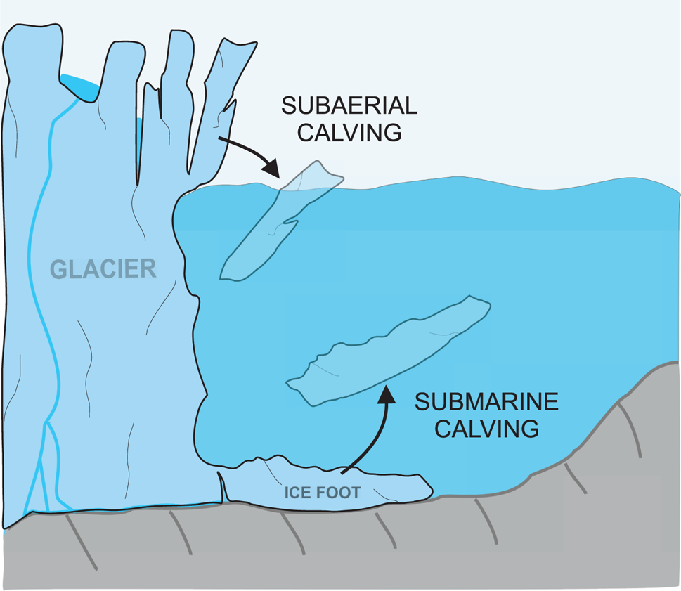
Fig. 1. Cartoon representing subaerial (SA) and submarine (SM) calving modes.
Russell (Reference Russell1891) provided one of the first descriptions of submarine calving events: ‘As the sea-cliff of ice recedes and the submerged terrace increases in breadth there comes a time when the buoyancy of the ice at the bottom exceeds its strength, and pieces break off and rise to the surface’. More than a century later, Hunter and Powell (Reference Hunter and Powell1998) reported the existence of an ‘ice terrace’ (or ‘ice foot’) at the front of Muir Glacier in Glacier Bay, Alaska. Several authors have observed broaching (i.e. rapidly surfacing) icebergs as much as few hundred meters beyond a glacier terminus (e.g. Warren and others, Reference Warren1995; Motyka, Reference Motyka1997; Hunter and Powell, Reference Hunter and Powell1998; Sugiyama and others, Reference Sugiyama, Minowa and Schaefer2019). Time-lapse observations of glacier termini have shown that usually only 2–15% of all calving events are submarine (e.g. Bartholomaus and others, Reference Bartholomaus, Larsen, O'Neel and West2012; Minowa and others, Reference Minowa, Podolskiy, Sugiyama, Sakakibara and Skvarca2018; How and others, Reference How2019). Nevertheless, studying submarine calving is important for three major reasons. First, despite their low occurrence, submarine calving events may still contribute significantly to frontal ablation because of the disproportionately large sizes of icebergs breaking off under the water. For example, Warren and others (Reference Warren1995) estimated that only 7% of all calving events observed at Glaciar San Rafael, Chile were submarine, but they accounted for ~27% of the total calving flux. Second, insight into any operating causal relationships between subaerial and submarine events may be important for formulating physics-based calving laws (van der Veen, Reference van der Veen2002; Benn and others, Reference Benn, Warren and Mottram2007; Bassis, Reference Bassis2011). Third, submarine calving events are hazardous for touristic cruises by boats and kayaks due to the sudden emergence of large icebergs up to several hundred meters from glacier termini (e.g. Purdie and others, Reference Purdie, Bealing, Tidey, Gomez and Harrison2016; Sugiyama and others, Reference Sugiyama, Minowa and Schaefer2019). However, detection of submarine calving events with standard glaciological methods is difficult due to several factors, including: (1) inability to use optical remote sensing (e.g. time-lapse cameras, satellites) to observe changes at submarine glacier termini, (2) significant drift of icebergs between consecutive time-lapse images caused by wind stress and water currents, (3) weak submarine calving seismicity (Bartholomaus and others, Reference Bartholomaus, Larsen, O'Neel and West2012; Köhler and others, Reference Köhler, Nuth, Schweitzer, Weidle and Gibbons2015, Reference Köhler2019) and (4) small relative volumes of the above-water expression of icebergs (low visibility). For example, How and others (Reference How2019) hypothesized that the ability to identify submarine events in time-lapse images of the glacier terminus can decrease rapidly with distance from the camera.
The use of underwater sound to identify submarine calving is explored here by combining underwater noise recordings and time-lapse images taken in the glacial bay of Hansbreen, Svalbard. Previous acoustic studies have demonstrated that ice mass loss due to subaerial calving can be quantified from the underwater noise of iceberg-water impact (Glowacki and others, Reference Glowacki2015; Glowacki and Deane, Reference Glowacki and Deane2020). Moreover, it was also hypothesized that submarine calving could be acoustically distinguishable from subaerial calving (Glowacki and others, Reference Glowacki2015). This hypothesis is validated here using a dataset of 656 subaerial and 162 submarine calving events observed in 2016 and 2017 at Hansbreen. Statistical and time–frequency analysis of the underwater noise demonstrates that subaerial and submarine calving events can be distinguished using two predictors: (1) the shape parameter of the log-normal distribution of the noise power and (2) the calving signal duration.
2. Study area
Hansbreen is a grounded, tidewater glacier terminating in Hornsund fjord, Svalbard (see Fig. 2). It has a 1.5 km wide calving terminus, total length of ~15 km and an area of more than 50 km2 (Błaszczyk and others, Reference Błaszczyk, Jania and Hagen2009, Reference Błaszczyk, Jania and Kolondra2013). The mean thickness and volume of the glacier are ~170 m and 9.5 km3 (Grabiec and others, Reference Grabiec, Budzik, Jania, Puczko and Kolondra2012). The typical water depth near the grounding zone and the average height of the ice cliff above the waterline are 60 and 38 m, respectively (Błaszczyk and others, Reference Błaszczyk2021). Consequently, more than 60% of the terminus surface area is submerged. Short-term velocities along the terminus of Hansbreen measured in 2015 with a terrestrial laser scanner averaged 0.8 m d−1; the glacier's movement is dominated by basal sliding (Jania, Reference Jania1988; Vieli and others, Reference Vieli, Jania, Blatter and Funk2004). The glacier retreated 917 m between 1992 and 2012; the average and maximum retreat rates during this period were 38 and 311 m a−1, respectively (Błaszczyk and others, Reference Błaszczyk2021). The highest retreat rates coincide with inflows of warm Atlantic waters to Hornsund fjord.

Fig. 2. (a) Map of the study site, (b, c) a pair of consecutive time-lapse images of the glacier terminus and (d) the corresponding underwater noise spectrogram with black arrows showing major submarine calving events (colorbar units in dB re 1 μPa2 Hz−1). Locations of time-lapse cameras and acoustic buoys are marked with orange and white font, respectively. Landsat 8 satellite data collected on 3 August 2017, courtesy of the US Geological Survey, Department of the Interior. Bathymetric data provided by (1) the Norwegian Hydrographic Service under the permit no. 13/G722, issued to the Institute of Geophysics, Polish Academy of Sciences and (2) the Faculty of Earth Sciences, University of Silesia in Katowice (see supplement to Błaszczyk and others, Reference Błaszczyk2021).
Vieli and others (Reference Vieli, Jania and Kolondra2002) proposed two major mechanisms controlling calving activity at Hansbreen: (1) instabilities driven by buoyancy forces due to changes in bed and glacier topography (height-above-buoyancy model; van der Veen, Reference van der Veen1996) and (2) melting at the waterline. They hypothesized that the heat flux supplied by the ambient fjord water causes thermal notching and break-off of the overhanging ice slabs. However, Pętlicki and others (Reference Pętlicki, Ciepły, Jania, Promińska and Kinnard2015) demonstrated that the calving depth (measured up-glacier) can be up to twice the undercut notch depth. This disproportion in ice loss is due to stress migration and is known as the ‘calving multiplier effect’ (O'Leary and Christoffersen, Reference O'Leary and Christoffersen2013; Benn and others, Reference Benn2017). Consequently, submarine melting is an important trigger of subaerial calving. Submarine calving events are also regularly observed (see Figs 2b, c; Jania, Reference Jania1988; Vieli and others, Reference Vieli, Jania and Kolondra2002; Glowacki and others, Reference Glowacki2015), suggesting the development of an underwater ice foot at the glacier terminus.
3. Data collection and analysis
3.1. Observation of calving events
Subaerial and submarine calving events are studied at Hansbreen using a combination of time-lapse photography and passive cryoacoustics. The study covers two observation periods of ~3 months each: (1) 21 July–26 October 2016 and (2) 15 June–22 September 2017. This subsection details the data collection process.
3.1.1. Time-lapse photography
Time-lapse images of the glacier terminus were taken every 15 min using a Canon EOS 1100D camera (4272 × 2848 pixels, 18 mm focal length) equipped with a Harbortronics Digisnap intervalometer (see ‘CAM’ in Fig. 2a). The camera system was powered with a solar panel and a 12 V DC battery. It was regularly visited by an observer in order to replace memory cards and to identify potential issues, including power cuts, clock drifts and fogging up of the front camera cover. Additionally, a higher frame-rate camera was required to validate the identification of submarine calving events in Canon images and to double-check the synchronization between photographic and acoustic data (clock drift). For this purpose, a GoPro Hero 3+ camera was set up closer to the calving terminus to take images every second in the initial phase of the study, i.e. from 21 July to 11 August 2016 (see ‘GoPro’ in Fig. 2a). The GoPro camera was not always active due to the lack of continuous supervision by the observer and the limited capacity of the SD card; high-frequency images covered 270 h during 22 d of camera operation (more than 12 h daily). Nevertheless, the low-frequency camera was usually sufficient in capturing submarine and subaerial calving events (with some ambiguity discussed below).
Calving events that could not be unambiguously identified on images and noise recordings were discarded. The ambiguity resulted mainly from three reasons: (1) the occurrence of rain, fog or clouds that lowered the quality of time-lapse images, (2) multiple calving events during a 15 min observation interval combined with a lack of high-frequency GoPro images and (3) lack of clear acoustic signatures that occurred for a limited number of events. Calving events were classified into two categories: subaerial (SA) and submarine (SM). The latter often produced debris-rich icebergs and usually involved only the submarine part of the glacier terminus. However, mixed events with clear evidence of additional subaerial break-up were also observed and classified to the SM category (with a note).
3.1.2. Underwater acoustic recordings
The noise measurements were made continuously at a sampling rate of 32 kHz using a Wildlife Acoustics SM3M Submersible recorder (discontinued) equipped with an HTI-96-MIN omnidirectional hydrophone with sensitivity of − 164 dB referenced to 1 V μPa−1 and a flat frequency response between 2 Hz and 30 kHz. The recorder was powered by lithium D-cell batteries. The uncompressed acoustic data were divided into 1 h segments and written onto SD cards.
Different deployment locations were selected for each of the measurement periods: ~1000 and 2000 m from the glacier terminus and at depths of 40 and 22 m, respectively in 2016 and 2017 (see ‘ACU_2016’ and ‘ACU_2017’ in Fig. 2a). Two experimental geometries were used to check if (and how) different propagation conditions and signal-to-noise ratios affect the acoustic classification of calving events into SA and SM categories.
3.2. Acoustic data analysis
The objective of the acoustic analysis is twofold: (1) to determine the start and end times of calving events in the acoustic recordings and then (2) to investigate properties of the calving noise. Details of the data processing are discussed below.
3.2.1. Determining time boundaries of calving signatures
A semi-automatic algorithm for determining start and end times of calving events in the acoustic record is implemented. The analysis covers only those calving events that were unambiguously identified in images (see Section 3.1.1). The objective is to start at the nominal middle of a calving signal and then to expand to the left and right. This expansion continues for as long as the noise level exceeds a chosen threshold value. Several user-provided parameters are required: t mid, f 0, f 1, Ψ, Γ and τmax (discussed below). The algorithm proceeds as follows:
(a) The nominal middle of a calving event, t mid, is manually selected based on visual and audible inspection of the acoustic waveform in Audacity – a free and open source software. A short 5 min segment of the acoustic pressure time series centered at t mid is taken for further analysis, 5 min being longer than the longest calving signature observed.
(b) A power spectral density estimate, P xx(t, f), of the 5 min noise segment is computed using a 8192-point fast Fourier transform with a 0.256 s Hamming window and a $50\percnt$
 overlap.
(c) A time series of the noise power, P(t), is computed by band-pass integrating P xx(t, f) from f 0 to f 1:
(1)$$P( t) = \int_{\,f_0}^{\,f_1}P_{xx}( t,\; f) \, {\rm d} f.$$The lower and upper integration limits were set to 30 and 200 Hz to maximize the signal-to-noise ratio for subaerial and submarine calving events.(d) A baseline power, P base(t), is calculated using a median filter of length Ψ = 40 s across all elements of P(t).
(e) A median filter of length Γ = 2.3 s is applied to P(t) to eliminate short noise impulses not related to calving events.
(f) Start and end times of a calving event, respectively t 0 and t 1, are calculated as follows. First, t 0 and t 1 are initially set to t mid. Second, t 0 is reduced as long as P(t) > 2P base(t) at any time during a preceding period of τmax = 12 s. The assumption is that noise signatures separated by more than τmax are not generated by a single calving event. Finally, an analogous procedure is used for t 1 but in the opposite direction. The calving signal duration, Δt, is obtained by subtracting t 0 from t 1.


Values of user-provided parameters were selected by visual inspection of the data and trial-and-error method (see Supplement for details). Different glaciers may require some local adjustments of these parameters for several reasons. For example, signal-to-noise ratios, activity of interfering sound sources, noise propagation conditions and size distributions of calved ice blocks in different locations are expected to be different at least to some extent. The semi-automatic procedure to determine t 0 and t 1 for subaerial and submarine calving events can potentially be made fully automatic; however, this would require a thorough investigation of different interfering noise sources. Examples of interfering sources include, for example, the low-frequency flow noise, energetic interactions between pieces of ice floating on the sea surface and disintegration of nearby icebergs. Moreover, an automatic detector should be tested and validated for both calving types (SA and SM) and different signal-to-noise ratios. For these reasons, the development of an event detection algorithm that would select t mid automatically requires (and deserves) a comprehensive analysis that lies beyond the scope of this study.
3.2.2. Time and frequency analysis of the calving noise
Start and end times of a given calving event are used to estimate its total noise energy. The analysis begins with the power spectral density of the acoustic signal (step (b) of the algorithm described in Section 3.2.1). The frequency-dependent calving noise power at the receiver is calculated by integrating P xx(t, f) over the event duration:

Then, the background noise power is estimated analogously using acoustic signal of the same length (Δt), recorded just before the corresponding calving event:

Finally, the total calving noise energy uncorrected for propagation losses is given by

where ρw is the water density, c w is the sound speed, 4π is the surface area of a unit sphere (over which the noise signal must be integrated to obtain total noise energy in joules) and f l and f u are lower and upper frequency limits, respectively. Unlike f 0 and f 1 that were introduced in Section 3.2.1, the integration limits in Eqn(4) are not constants but variables. Different values of f l and f u are applied in Section 4.3. In the case of subaerial calving, E ac,obs was previously found to be correlated with the kinetic energy of the falling ice block and the calving signal duration (see supplement of Glowacki and Deane, Reference Glowacki and Deane2020). Therefore, in order to emphasize potential differences in acoustic signatures of SA and SM events and not the variability in block sizes, the total calving noise energy is divided by the event duration:

Equation (5) gives an estimate of the average calving noise power. The analysis of the time-varying calving noise power is also required. For this purpose, the power spectral density estimated for t 0 ≤ t ≤ t 1 is integrated over f l and f u:

As in Eqn (4), f l and f u are not necessarily the same as f 0 and f 1 that were used in Eqn (1). Finally, the min–max normalized calving noise power is given by

4. Results and discussion
4.1. Calving inventory
Table 1 summarizes observations of calving events made during the experiments. A total of 393 and 425 events were unambiguously identified on the acoustic record and time-lapse images, respectively in 2016 (period I) and 2017 (period II).
Table 1. Number of observed calving events divided into mode

Subaerial calving events accounted for 78 and $83\percnt$ of all observations, respectively in periods I and II. However, the event detection procedure discarded more SA events than SM events; this disproportionality resulted from a typically higher abundance of subaerial events between two consecutive time-lapse images (ambiguity issue; see Subsection 3.1.1). It is, therefore, very likely that SM events at Hansbreen are in fact 8–10 times less frequent than SA events. This observation is consistent with previous reports from Alaska (Bartholomaus and others, Reference Bartholomaus, Larsen, O'Neel and West2012), Patagonia (Minowa and others, Reference Minowa, Podolskiy, Sugiyama, Sakakibara and Skvarca2018), Greenland (Minowa and others, Reference Minowa2019) and other glaciers in Svalbard (How and others, Reference How2019). However, images from time-lapse cameras demonstrated that – despite their rarity – submarine events often produced voluminous icebergs that quickly filled out a significant portion of the glacial bay (see panels b and c in Fig. 2). Determining the contribution of SM events to the total calving flux from Hansbreen lies beyond the scope of this study. Nevertheless, time-lapse observations reported here provide some evidence that submarine calving may be an important process of ice loss at the glacier–ocean boundary and cannot be neglected. This should not come as a surprise as the submarine portion of the glacier terminus is usually much larger than the subaerial portion (a factor of 1.6 at Hansbreen). Similar conclusions were drawn, for example, by Warren and others (Reference Warren1995) and Motyka (Reference Motyka1997).
Interestingly, submarine events that produced growlers extending ${\lesssim }0.5$ m above the sea surface often stayed undetected by the distant, low-frequency camera. This issue was revealed by high-frequency GoPro images taken at a much closer position and bare-eye observations made during short boat trips close to the glacier terminus (250–500 m). Ice blocks released underwater are often darker than subaerial ice due to their high sediment content; therefore, it is usually harder to identify small pieces of submarine ice floating at the sea surface. Moreover, other factors also hinder the observation of SM events: (1) the lack of changes at the visible part of the terminus, (2) glare of the fjord surface and (3) long separation (15 min) between the consecutive images combined with strong surface currents in the bay. At times it was also impossible to identify low-magnitude submarine events on the acoustic record; it is likely because of their low energy of ice/ocean interactions. The same issue existed for small pieces of ice breaking off at the waterline.
Submarine events were sometimes accompanied by the break-off of ice from above the waterline. These ‘mixed’ detachments accounted for 12.5 and 15% of all SM events, respectively in 2016 and 2017 (see Table 1). The co-existence of SA and SM events may indicate a causal relationship between these two calving modes. In support of this hypothesis, O'Neel and others (Reference O'Neel, Marshall, McNamara and Pfeffer2007) suggested that the release of submarine ice blocks can be driven by the sudden reduction of the overburden pressure that leads to the increase of the buoyancy forces acting on the ice foot. However, a quantitative study of this phenomenon would require a continuous record of high-frequency and high-resolution time-lapse images covering the entire calving terminus.
4.2. Underwater noise emission from subaerial and submarine calving
Figure 3 shows time-averaged spectra of the caving signal (‘SA’/‘SM’, blue/red ) and background noise (‘BG’, black) recorded in 2016 (a) and 2017 (b). Calving events are categorized into two modes: subaerial (‘SA’, blue) and submarine (‘SM’, red). The shading indicates the 25th and 75th percentiles, and the thick lines represent the median values.

Fig. 3. Time-averaged spectra of subaerial calving (SA), submarine calving (SM) and background noise (BG) computed using Welch's overlapped segment averaging estimator (Welch, Reference Welch1967). The calving inventory is separated into two periods with different hydrophone locations: period I (2016 – close buoy, panel a) and period II (2017 – distant buoy, panel b). Thick lines show median values and color shadings represent percentiles 0.25 and 0.75.
The difference between background noise and calving signal generated by SA and SM events is most evident between 10 Hz and ~500 Hz; the power spectral density usually peaks below 200 Hz. At frequencies higher than 500 Hz, the noise spectrum is almost certainly dominated by the underwater noise from submarine melting of the glacier terminus and nearby icebergs/growlers (see, e.g. Deane and others, Reference Deane, Glowacki, Tegowski, Moskalik and Blondel2014; Pettit and others, Reference Pettit2015). The melt noise results from an explosive release of pressurized gas bubbles as the ice melts (Scholander and others, Reference Scholander, Kanwisher and Nutt1956; Urick, Reference Urick1971). Importantly, at frequencies below 200 Hz the calving noise level is on average at least 20 dB (a factor of 100 in energy) higher than the background noise level. Consequently, calving events that are included in the inventory were easily identified in the audio recordings, regardless of their type (SA or SM).
Subaerial calving events are usually associated with higher noise levels than submarine calving events; however, this effect is much less pronounced at more distant buoy used in 2017 (compare panels a and b in Fig. 3). Moreover, the shape of the noise spectrum seems to be largely influenced by the frequency-dependent loss of the noise energy. For example, the noise spectrum at frequencies between 100 and 200 Hz is remarkably different for the close buoy and distant buoy (panels a and b of Fig. 3, respectively). Two factors are almost certainly responsible for these differences in noise spectra: (1) the variable thermohaline structure in the bay and (2) range-dependent bathymetry and sediment properties (see, e.g. Glowacki and others, Reference Glowacki, Moskalik and Deane2016). Glowacki and others (Reference Glowacki2015) hypothesized that the shape of the noise spectra may be used to distinguish between subaerial and submarine calving; however, the study investigated a limited number of events (10 SA and 2 SM). Here, the analysis of much more extensive calving inventory shows that the spectral slope of the noise generated by subaerial and submarine calving events is similar; this is true for both study periods at different distances. It clearly demonstrates two issues. First, the previous study did not fully capture the variability in noise emission from calving because of the small sample size. Second, the analysis of calving noise designed to distinguish between SA and SM events should not be limited to the frequency domain. The latter issue will now be addressed through the analysis of the time and frequency structure of the calving noise.
The time–frequency analysis is based on spectrograms of the calving noise. Typical spectrograms of the underwater noise from subaerial and submarine calving are shown, respectively, in panels a and b of Fig. 4. For the SA event in Fig. 4a, the highest acoustic energy is generated over a short time period between 7 and 13 s. Distinct sound-source mechanisms are active in this stage, including: (1) initial impact and momentum transfer to the water column (see ~7 s in the spectrogram; timing from synchronized GoPro images), (2) air entrainment, (3) collective oscillation of a bubble plume and (4) secondary impacts due to splashes (Glowacki, Reference Glowacki2020). This period is followed by the calving-induced surface wave action that generates noise at frequencies between 20 and 200 Hz (see noise energy exceeding the background level after 15 s). The noise spectrogram computed for the SM event in Fig. 4b is remarkably different. First, there are no clear signatures of mini-tsunami waves. This is in line with large-scale laboratory experiments reported by Heller and others (Reference Heller2019); buoyancy-driven calving events usually generate surface waves of much smaller amplitude in comparison with gravity-driven falls. Second, and most importantly, isolated transients lasting usually <1 s dominate the time and frequency structure shown in Fig. 4b (see short energy bursts at, e.g. 3, 24 and 26 s). Possible sound-source mechanisms in submarine calving include, for example, ice fracturing, cracking, block detachment and broaching. The noise transient evident at ~13 s of the spectrogram coincided in time with the emergence of the ice block (as captured by the GoPro camera). However, it is not a general rule. Sometimes the ‘broaching phase’ was acoustically undetectable. This is not at all surprising, given that the noise emission during broaching almost certainly depends on the ice block volume and its ascending velocity; these two variables determine the kinetic energy of the ice block during its interaction with the sea surface. Simple model calculations were done to estimate the velocity of a rising iceberg (not reproduced here). The iceberg should not reach its terminal velocity if the water depth is <100 m; therefore, the maximum upward velocity of submarine icebergs observed at Hansbreen is almost certainly related to the detachment depth. Consequently, low-magnitude submarine events that originate in shallow water do not generate much noise during the broaching phase.

Fig. 4. Comparison of the time and frequency structure of the noise generated by representative examples of subaerial and submarine calving events. (a, b) Spectrograms of the power spectral density estimates (colorbar units in dB re 1 μPa2 Hz−1). (c, d) Time series of the normalized noise power. (e) Plots of ECDFs of the noise power. The integration limits were set to f l = 10 Hz and f u = 500 Hz. Black dashed lines in panels c and d indicate estimated start and end times of the calving signal (t 0 and t 1, respectively), which were used to compute ECDFs shown in the panel e.
The difference in noise emission between SA and SM events is also demonstrated in panels c and d of Fig. 4. The plots show min–max normalized noise power calculated using Eqn(7). In order to focus on the ‘calving band’, lower and upper integration limits were set to f l = 10 Hz and f u = 500 Hz, respectively (recall a wide peak in the frequency spectrum of the calving noise; Fig. 3). The normalized noise power during the subaerial event does not fall below 10−1 for a continuous period of ~5 s. This suggests an overlap in time between different but closely associated sound-source mechanisms. In contrast to that, the noise power during the submarine event only occasionally rises above 10−1; individual peaks are clearly separated and distributed over a much longer event duration of ~25 s. Finally, plots of empirical cumulative distribution functions (ECDFs) of the normalized power are shown in panel e. The different shapes of the curves indicate a clear difference in the temporal distribution of noise energy between SA and SM events. For example, note a much steeper slope (more frequent occurrence) for 10−3 ≤ P′ ≤ 10−2 in the case of submarine calving, which demonstrates that the noise power is low for a large percentage of the time.
The following section aims to identify calving noise properties that can be used to distinguish acoustically between subaerial and submarine calving. For this purpose, the distribution of the calving noise power and other noise characteristics will be investigated through a statistical analysis of calving noise using the entire calving inventory.
4.3. Calving noise statistics
The statistical analysis of the calving noise starts with two questions: (1) Do the differences in noise emission from SA and SM calving (identified in Section 4.2) hold for the entire dataset? and (2) What distribution does P′ come from? First, time series of the noise power were calculated individually for all calving events observed in the summer of 2016 and categorized by event type (period I; see Table 1). Figure 5a shows collective histograms of the normalized calving noise power computed separately for subaerial and submarine events.

Fig. 5. Histograms of min-max normalized noise power computed for calving events observed in 2016. The integration limits were set to f l = 10 Hz and f u = 500 Hz. Raw and log-transformed variables were used in plots a (left) and b (right), respectively. Color lines show probability density estimates computed using Matlab's kernel smoothing function estimate (ksdensity; Hill, Reference Hill1985). Note the logarithmic scale on the vertical axis of the plot a.
Distributions of P′ are non-Gaussian and right-skewed for both calving types. The occurrence of P′ > 0.4 is more frequent for subaerial events than for submarine events. In order to emphasize possible differences in noise emission between SA and SM events for P′ < 0.2, a natural logarithmic transformation was applied. However, to make this transformation possible, the minimum value of the normalized power for each calving event (i.e. P′ = 0) was excluded from analysis. Histograms of logP′ are shown in Fig. 5b. Most importantly, distributions of the log-transformed normalized noise power are different for subaerial and submarine events. This observation suggests that SA and SM events could potentially be distinguished. The probability density function estimated for submarine calving events peaks between − 5 and − 2. The number of occurrences in this range of values is much higher than in the case of SA events. In contrast, the logarithm of the normalized power for subaerial events is more often lower than − 5.5 and the spread of values around the mean is higher. Moreover, the shapes of the probability density functions after the transformation closely resemble the famous bell-shaped curve of the Gaussian distribution. Consequently, the normalized power estimated for individual calving events may be log-normally distributed (Gaddum, Reference Gaddum1945). This interesting possibility will now be explored.
The null hypothesis that the log-transformed normalized noise power comes from a normal distribution was tested at a $1\percnt$ significance level using a one-sample Kolmogorov–Smirnov test; the distributions of logP′ calculated for all individual calving events were used in this analysis. Different integration limits were applied to calculate P′: 10 Hz ≤ f l ≤ 500 Hz and 150 Hz ≤ f u ≤ 1000 Hz. The step in frequency was 50 Hz for frequencies greater than or equal to 50 Hz. The primary reason behind testing different values of f l and f u is to identify the integration limits that result in the least similarity between distributions of P′ calculated for subaerial and submarine events. On average, the null hypothesis could not be rejected at a given significance level for 85 and $93\percnt$
 of calving events observed in 2016 and 2017, respectively. The calving noise power at Hansbreen is, therefore, usually log-normally distributed. That should not come as a surprise given the omnipresence of the log-normal distribution in science; examples include Earth sciences, medicine, economics and social sciences (e.g. Limpert and others, Reference Limpert, Stahel and Abbt2001). Importantly, the log-normal distribution of the calving noise power shows differences between subaerial and submarine events (see Figs 4e, 5). The next step is to explore the differences in power distributions to see if they can be used to distinguish between the two calving modes.
There are two major parameters of the log-normal distribution: it's mean μ and standard deviation σ, which will be referred to as the scale and shape parameters respectively. The distribution parameters were calculated for all calving events using the same integration limits that were used for the null hypothesis testing (i.e. 10 Hz ≤ f l ≤ 500 Hz and 150 Hz ≤ f u ≤ 1000 Hz). Additionally, the average power of the calving signal, $\bar {P_{\rm c}}$ , was also calculated for each calving event and each pair of f l and f u values using Eqn (5). Then, the probability density functions of parameters σ, μ and $\log _{10}\bar {P_{\rm c}}$
 were estimated separately for different calving types (SA and SM) and integration limits (f l and f u) using Matlab's kernel smoothing function (ksdensity; Hill, Reference Hill1985). The area created by the overlap between two probability density functions estimated for subaerial and submarine events and multiplied by 100$\percnt$
 was adopted as a measure of similarity in parameter values between the two calving modes. The overlapped area was calculated by taking the minimum value of two probability density functions at each point and then integrating the resulting function over the entire range (using the trapezoidal rule). The results obtained for period I (2016) are shown in panels a–c of Fig. 6. The shape parameter shows the least similarity and provides the best discrimination between calving modes; the similarity between probability density functions is as low as 21$\percnt$
 for f l = 200 Hz and f u = 650 Hz (see the pink dot in panel a). The similarity measure stays below 38$\percnt$
 for f u ranging from 300 to 900 Hz (with an average of $27\percnt$
 ). For μ and $\log _{10}\bar {P_{\rm c}}$
 , similarities are higher but still low enough to be significant: average similarities are 63 and 42$\percnt$
 , respectively. Figure 6, panels d–f show probability distribution functions estimated for the parameters σ, μ and $\log _{10}\bar {P_{\rm c}}$
 computed with integration limits of f l = 200 Hz and f u = 650 Hz (to maximize differences for σ). Modal values of the most distinctive shape parameter are ~1 and 1.5, respectively for submarine and subaerial events. The similarity between parameters calculated for SA and SM events observed in 2017 is higher than in the case of 2016 data (see Supplement for details); this observation suggests that distinguishing calving types is more difficult when the acoustic receiver is deployed farther from the glacier terminus (see positions of the buoys in Fig. 2a).
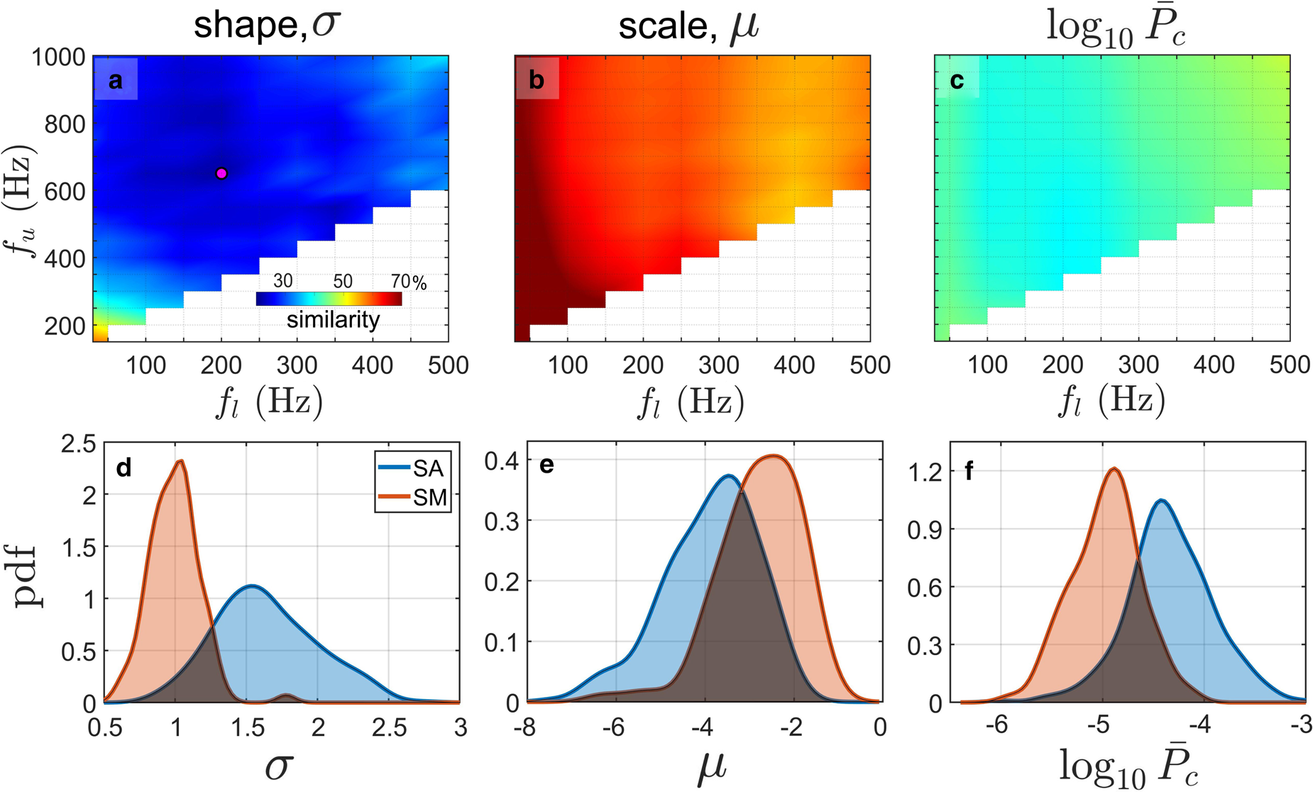
Fig. 6. (a–c) Color plots of the similarity between probability density functions of parameters σ, μ and $\log _{10}\bar {P_{\rm c}}$ calculated for SA and SM events observed in 2016. Variables f l and f u denote lower and upper integration limits, respectively. (d–f) Probability density functions estimated for the noise parameters using Matlab's kernel smoothing function (ksdensity; Hill, Reference Hill1985); f l = 200 Hz and f u = 650 Hz (pink dot in panel a). Dark areas indicate overlaps between probability density functions used as a similarity measure in panels a–c.
The time and frequency analysis of the noise generated by representative examples of SA and SM events suggested that typical signal duration may also be different for the two calving modes (see Section 4.2; Fig. 4). Indeed, this is demonstrated in Fig. 7 that shows probability density functions of Δt calculated for calving events observed in 2016 and 2017 using the semi-automatic algorithm (see Section 3.2 and Supplement for details). The overlap between probability distribution functions is $58\percnt$ for period I and $41\percnt$
 for period II. Typical calving signal duration is ~10 and 20 s, respectively for subaerial and submarine events. Longer acoustic emission from SM events almost certainly reflects larger time intervals between individual sound-source mechanisms. For example, the separation in time between the ice block detachment at depth and its appearance on the sea surface is expected to be longer in comparison with the duration of the free ice fall. Moreover, ice cracking and fragmentation taking place underwater are expected to be much easier to detect acoustically in the water column than ice detachment from above the water.

Fig. 7. Probability density functions estimated for the duration of the calving noise generated by subaerial (SA, blue) and submarine (SM, orange) calving events. The estimate was computed using Matlab's kernel smoothing function (ksdensity; Hill, Reference Hill1985).
A total of four parameters have been identified as potentially useful in acoustic differentiation between submarine and subaerial calving: (1–2) shape and scale parameters of the log-normal distribution of the normalized calving noise power, (3) the average calving noise power and (4) the calving signal duration. These parameters will be used in the following section to test if the acoustic classification of glacier calving into SA and SM categories is feasible.
4.4. Classification of the calving mode
Figure 8 shows scatterplots of the parameter σ and other parameters of the calving noise discussed in Section 4.3. Black dashed lines indicate fitted discriminant analysis models computed by minimizing the expected classification cost for SA and SM events (Matlab's function fitcdiscr). In 2016, all parameters paired with σ allow most submarine and subaerial events to be distinguished (Figs 8a–c). The percentage of misclassifications is not higher than 5 and $20\percnt$ for SA and SM events, respectively. In 2017, classifying calving events with similar effectiveness (as in 2016) is possible only when combining the parameter σ and the signal duration (Figs 8d–f). The lower classification performance of parameters μ and $\log _{10}\bar {P_{\rm c}}$
 for data collected in 2017 is especially pronounced for subaerial events and almost certainly results from a greater distance between the buoy and the glacier terminus that lowered the signal-to-noise ratio. Values of parameters σ and Δt seem to be least sensitive to the receiver location. Interestingly, parameters computed for submarine events that contained the break-off of ice also from above the waterline (‘mixed events’) usually have values typical for SM class and do not create a separate cluster (see red circles and triangles in Fig. 8).

Fig. 8. Relationship between the shape parameter (σ) of the log-normal distribution and other parameters of the calving noise generated by subaerial (SA, blue) and submarine (SM, orange) calving events observed in 2016 (a–c) and 2017 (d–f). Red circles and triangles indicate submarine events that contained the break-off of ice also from above the waterline (‘mixed events’). Black dashed lines show fitted discriminant analysis models computed using Matlab by minimizing the expected classification cost (function fitcdiscr).
The following procedure was applied to quantify the performance of the event classification into submarine and subaerial categories. First, the parameters σ and Δt were selected as predictors. The parameters μ and $\log _{10}\bar {P_{\rm c}}$ were not used due to their low classification performance in the case of the 2017 data (see panels d and f in Fig. 8). Second, the classification model shown in panels b and e of Fig. 8 has been modified in such a way that all calving events with Δt < 10 s are classified as subaerial (see red line in Fig. 9). The final model takes the following form:

The linear discrimination analysis was selected for simplicity. Moreover, the more sophisticated techniques (e.g. decision tree, support vector machine) were found to be less or similarly efficient in distinguishing SA and SM events. In order to test the performance of the classification model, n = 100 events were randomly selected from the calving inventory k = 20 000 times and classified into SA or SM categories using Eqn (8). Then, a true positive rate (TPR; sensitivity/recall), true negative rate (TNR; specificity/selectivity) and positive predictive value (PPV; precision) for subaerial and submarine events were calculated as follows:


where TP – true positives, FN – false negatives, TN – true negatives and FP – false positives. The analysis was performed separately for the 2016 data, 2017 data and total calving inventory. The results are shown in Fig. 10. The model performs very well in terms of classification of the event type. In the case of the total calving inventory, median values of the true positive rate are 90 and 84$\percnt$ , respectively for subaerial and submarine events (Fig. 10c). Typical TPRs are not lower than $78\percnt$
 (percentile 0.25 for SM events). The spread of TPR values is much lower for SA events. The box plots of TNRs demonstrate that – in the case of the 2016 data – the current classification model gives more false positives for SA events than SM events (Fig. 10d). However, the model could be easily adjusted to provide higher sensitivity (TPR) for submarine events at the expanse of lower specificity (TNR). Importantly, a greater distance between the buoy and the glacier terminus in 2017 results in a much lower precision (PPV) for SM events (see Fig. 10g–i); median values of PPV are 80 and $58\percnt$
 for the close buoy (2016) and more distant buoy (2017), respectively. This observation is in line with the previous analysis of the scatterplots between the calving signal duration and the parameter σ of the log-normal distribution of the noise power (compare panels b and e of Fig. 8). Typical values of the parameter σ estimated for the calving noise generated by SA and SM events are more similar when the receiver is placed farther from the glacier; this is almost certainly due to the decrease of the signal-to-noise ratio (see also Fig. 3) and frequency-dependent loss of the calving noise energy (see, e.g. Glowacki and others, Reference Glowacki, Moskalik and Deane2016). Therefore, the choice of locations for acoustic receivers is of key importance for the efficiency of the calving mode discrimination model. The following section covers future needs and possibilities regarding the long-term acoustic monitoring of calving; the topic is discussed in light of the new findings.

Fig. 9. Scatterplot of the calving signal duration and the shape parameter of the log-normal distribution of the normalized noise power estimated for subaerial and submarine calving events observed in 2016 (circles) and 2017 (triangles). Black and red lines represent the preliminary and final classification models, respectively.
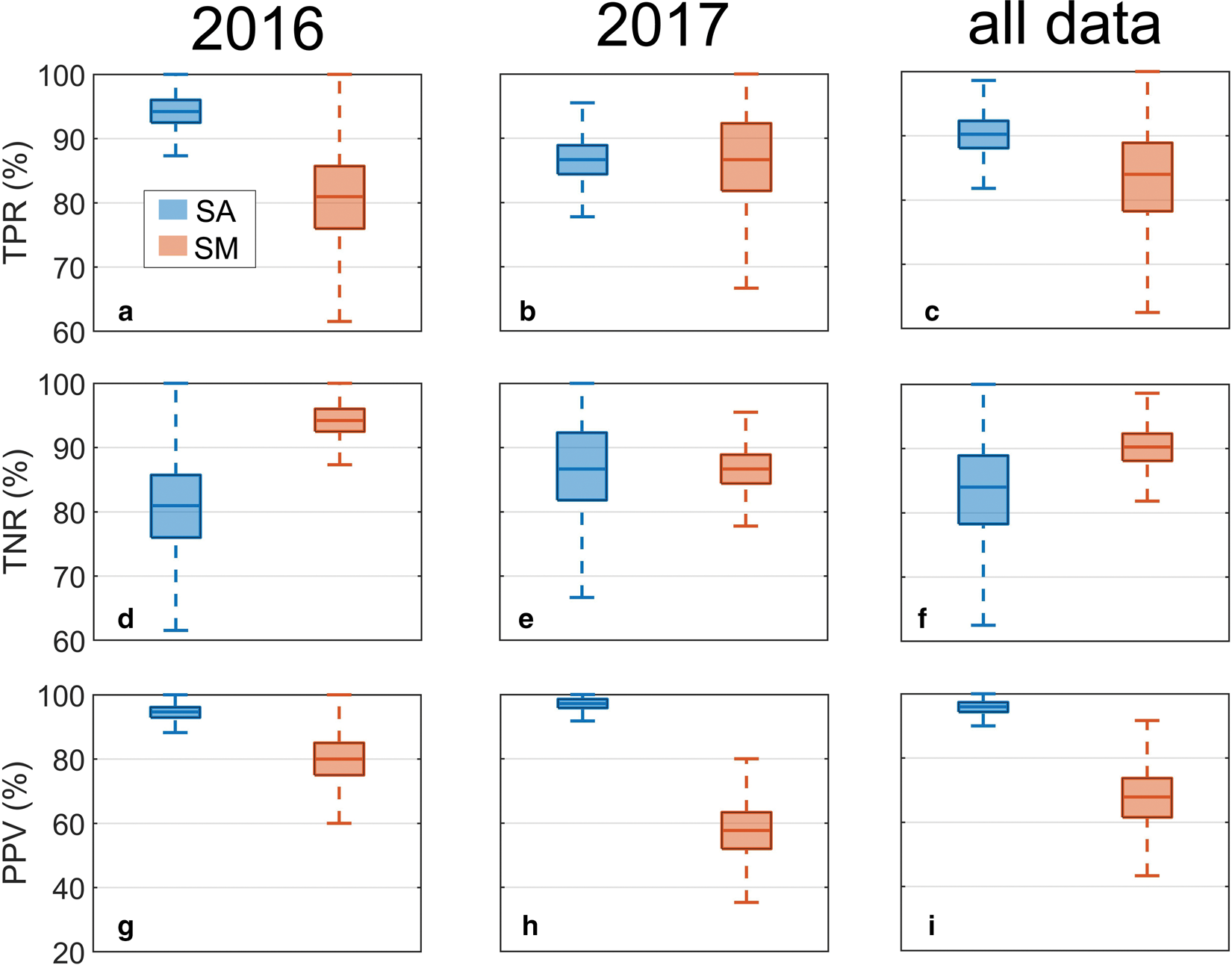
Fig. 10. Box plots of the true positive rate (sensitivity/recall; a–c), true negative rate (specificity/selectivity; d–f) and positive predictive value (precision; g–i) of the classification model computed by randomly selecting 100 events from the calving inventory (20 000 times). The analysis was performed separately for the 2016 data, 2017 data and total calving inventory. Boxes are limited by the 0.25 and 0.75 percentiles. Thick horizontal lines and vertical whiskers show median and extreme values, respectively.
5. Long-term acoustic monitoring of calving
Recent studies have demonstrated that subaerial calving fluxes can be quantified through the analysis of the underwater noise from the impact of icebergs on the sea surface (Glowacki and others, Reference Glowacki2015; Glowacki and Deane, Reference Glowacki and Deane2020). The study presented here extends this work and shows that subaerial and submarine calving events can be distinguished acoustically with a high degree of accuracy if the acoustic recordings are made within 2 km of the glacier terminus. If this result for Hansbreen translates to other glacial systems, the ice mass loss due to calving could potentially be divided into its aerial and underwater components. In addition to the potential of ice mass loss monitoring, the classification of calving events would allow for the study of any causal relationship between SM and SA calving. However, further scientific advances are required in order to use passive cryoacoustics as a practical tool to quantify and partition the solid ice discharge from marine-terminating glaciers, and these are discussed below.
First, underwater noise recordings should be taken in different locations and different glaciological settings. This is essential to answer two questions: (1) How site-specific are the properties (e.g. statistics, variability) of the calving noise? and (2) How do these properties change with variable glacier dynamics and geometry? The required data should not be too difficult to obtain. Acoustic recorders are relatively inexpensive, provide continuous data, do not require human supervision and can be attached to already existing moored systems. For example, passive cryoacoustics could be incorporated into a Greenland Ice Sheet-Ocean Observing System (GrIOOS; see Straneo and others, Reference Straneo2019) and a Svalbard Integrated Arctic Earth Observing System (SIOS). In fact, underwater noise recordings have been taken at close proximities to tidewater glaciers in Greenland (e.g. Podolskiy and Sugiyama, Reference Podolskiy and Sugiyama2020; Podolskiy and others, Reference Podolskiy, Murai, Kanna and Sugiyama2022), Alaska and Antarctica (e.g. Pettit and others, Reference Pettit2015; Zeh and others, Reference Zeh, Pettit and Wilson2017) and other fjords in Svalbard (e.g. Sanjana and others, Reference Sanjana, Latha, Thirunavukkarasu and Venkatesan2018; Köhler and others, Reference Köhler2019). However, the application of any existing or new acoustic datasets to verify the calving mode discrimination model will also require photogrammetric data.
Second, an efficient signal processing chain needs to be developed in order to analyze long-term acoustic datasets. This includes, for example, the creation of an automatic calving signal detector that would need to meet at least two criteria: (1) the ability to detect both subaerial and submarine events and (2) the ability to work well in variable background noise conditions (i.e. variable signal-to-noise ratios). The development of an automatic calving detector was beyond the scope of this study. Moreover, modern machine learning algorithms will likely be valuable in distinguishing a large number of subaerial and submarine events captured by long-term acoustic monitoring systems.
Finally, a better understanding of the sound-source mechanisms arising from submarine calving is required to explain the complicated time and frequency structure of the generated noise (see spectrogram in Fig. 4b). A preliminary work has already been done for subaerial calving (see Glowacki, Reference Glowacki2020), but the problem of submarine calving is obviously more challenging due to the difficulty in observing underwater iceberg detachments. Better insight into noise generation mechanisms is essential to link (currently unavailable) direct measurements of submarine calving fluxes with their corresponding underwater noise signatures. For this purpose, passive cryoacoustics will have to be combined with other remote-sensing techniques (e.g. active acoustics, radar interferometry, laser scanning).
6. Concluding remarks
This study combines passive cryoacoustics and time-lapse photography to investigate subaerial and submarine calving at Hansbreen, Svalbard in the summers of 2016 and 2017. Two major findings are presented: (1) the normalized calving noise power is log-normally distributed regardless of the calving style and (2) subaerial and submarine calving events can be distinguished acoustically. Two parameters of the calving noise are estimated for 656 subaerial and 162 submarine calving events and used as predictors: calving signal duration (Δt) and the shape parameter of the log-normal distribution (σ). The new methodology for classification of calving styles may be used for two purposes: (1) to find causal relationships between subaerial and submarine calving and (2) to partition the solid ice discharge from tidewater glaciers into aerial and submarine components.
Several conditions must be met before the discrimination model developed here can be broadly applied. First, an automated calving signal detector capable of identifying both subaerial and submarine events needs to be developed. Second, better understanding of the time and frequency structure of the calving noise and the corresponding sound-source mechanisms is required. Third, the ice mass loss due to submarine calving should be linked to the associated noise emission. Finally, the newly developed event classification model needs to be tested in different locations and glaciological settings, which will allow for a more thorough analysis of the model sensitivity and a detailed investigation of the variability of calving noise parameters. Moreover, I speculate that modern machine learning techniques may enable further improvement in the event classification performance and scope of its applicability if the calving inventory is much larger than the one presented here.
Supplementary material
The supplementary material for this article can be found at https://doi.org/10.1017/jog.2022.32.
Acknowledgements
I thank Grant Deane for providing very insightful comments and discussions and Mateusz Moskalik for his efforts in maintaining oceanographic and photographic monitoring during the study period. I am also grateful to Aleksandra Stępień and Adam Słucki from the HańczaTech diving team for their help in deploying and recovering of the acoustic buoys. The support from the wintering staff of the Polish Polar Station Hornsund is also greatly appreciated. Mandar Chitre, Hari Vishnu and Dale Stokes provided useful suggestions about the calving signal analysis. I also thank Bernd Kulessa (Scientific Editor), Evgeny Podolskiy, Jason Amundson and an anonymous reviewer for their insightful and detailed comments on the original version of the manuscript. The study was funded by the Polish Ministry of Science and Higher Education (grant no. 1621/MOB/V/2017/0 – ‘Mobility Plus’ programme and a subsidy for the Institute of Geophysics, Polish Academy of Sciences) and the US National Science Foundation (grant no. OPP-1748265). The monitoring data from the Polish Polar Station Hornsund are freely available at https://dataportal.igf.edu.pl/.


 Open access