Introduction

The Earth’s climate has always been characterized by natural variability. However, the global mean annual air temperature showed significant increase during the 20th century (Reference Parry, Canziani, Palutikof, Van der Linden and HansonParry and others, 2007). Glaciers are highly sensitive to variations in temperature and precipitation (Reference OerlemansOerlemans, 2005) and have therefore served as indicators of climate change in recent centuries (Reference Oerlemans and FortuinOerlemans and Fortuin, 1992; Reference Haeberli, Maisch and PaulHaeberli and others, 2002). The majority of glaciers throughout the world are retreating, with particularly pronounced retreating trends in mountain and valley glaciers (Reference Dyurgerov and MeierDyurgerov and Meier, 2000; Reference BarryBarry, 2006). This retreat was intensified at the end of the last century (Reference Khromova, Dyurgerov and BarryKhromova and others, 2003; Reference Paul, Huggel and KääbPaul and others, 2004a,Reference Paul, Kääb, Maisch, Kellenberger and Haeberlib). Most of the examined glaciers in the Tibetan Plateau have retreated to some extent, although a small number of glaciers continue to advance (Reference LiuLiu and others, 2006; Reference YaoYao and others, 2012). Many studies have reported accelerations in glacial retreat in recent years due to increased air temperature and change in the partitioning of precipitation (more rain than snow at high elevations), which have resulted in negative glacier mass balance (Reference Yao, Pu, Lu, Wang and YuYao and others, 2007; Reference Kang, Xu, You, Flügel, Pepin and YaoKang and others, 2010). This retreat affects river runoff regimes (Reference Yao, Wang, Liu, Pu, Shen and LuYao and others, 2004; Reference LiuLiu and others, 2006) and glacier outburst floods and mudflows in the upper valleys (Reference GlantzGlantz, 1999). In the Tibetan Plateau, the glacial retreat is most pronounced in the Yigong Zangbo basin (YZB), where glacier length has decreased at a rate of 48 m a⁻¹ and glacial area has reduced at a rate of 0.57% a⁻¹ between 1971 and 2000 (Reference YaoYao and others, 2012). The changes in the glaciers of the YZB and of the entire Tibetan Plateau can be monitored as an indicator of continuing climate change (Reference Niederer, Bilenko, Ershova, Hurni, Yerokhin and MaselliNiederer and others, 2008).

Mass-balance measurements provide a direct signal (i.e. a signal with no time delay) of the effects of climate change on variations in glacial accumulation and ablation (Reference Kaser, Cogley, Dyurgerov, Meier and OhmuraKaser and others, 2006; Reference Berthier, Arnaud, Kumar, Ahmad, Wagnon and ChevallierBerthier and others, 2007). Estimating the flow velocity of valley glaciers is very important in understanding the glacier mass balance, as the discharge of ice mass is largely dependent on the glacier velocity, with accelerated or decreased motion indicating an alteration of the ice mass equilibrium (Reference Nakamura, Doi and ShibuyaNakamura and others, 2007; Reference Strozzi, Kouraev, Wiesmann, Wegmüller, Sharov and WernerStrozzi and others, 2008). Knowledge of the seasonal and interannual variability of the velocity is important for understanding the response of glaciers and ice caps to expected climate change. In particular, glacier velocities provide information on the potential effects on water resources, sea-level rise and glacier-related hazards (Reference Dowdeswell, Unwin, Nuttall and WinghamDowdeswell and others, 1999; Reference BerthierBerthier and others, 2005). Although in situ observations can provide highly accurate glacier velocity determinations, it is not feasible in practice to visit remote glacier areas frequently. Given the difficulty of direct field-based monitoring of glaciers in remote areas, satellite remote sensing is an attractive approach for monitoring changes in the surface movement of glaciers (Reference Joughin, Winebrenner and FahnestockJoughin and others, 1995) and ultimately for estimating changes in the mass balance of glaciers. Glacier monitoring using optical remote sensing is limited by the strong weather patterns characteristic of glacierized areas, including thunderstorms, rain and snowfall, all of which cause frequent and rapid changes in illumination. In addition, it is difficult to obtain cloudless optical data for these regions on a regular basis, which are required for a robust monitoring of glacier flow patterns. In contrast, synthetic aperture radar (SAR) imagery has several advantages over other remote-sensing approaches, including the ability to observe through cloud cover, and its insensitivity to variations in weather or illumination.

The SAR interferometry (InSAR) method is a valuable technique for studying glacier dynamics, due to its high sensitivity to terrain deformations (Reference Joughin, Smith and AbdalatiJoughin and others, 2010; Reference Gourmelen, Kim, Shepherd, Park, Sundal and BjörnssonGourmelen and others, 2011). Both conventional InSAR and multiple aperture InSAR (MAI) require effective interferometry to obtain accurate results (Reference Bechor and ZebkerBechor and Zebker, 2006; Reference Gourmelen, Kim, Shepherd, Park, Sundal and BjörnssonGourmelen and others, 2011). Satellite radar feature tracking (SRFT), however, does not demand the interferometry condition, i.e. there are no strict limitations on the time interval and spatial baseline length of the SAR image pairs, as long as there are images in the detecting areas (Reference Scherler, Leprince and StreckerScherler and others, 2008). The main advantage of SRFT over InSAR is the fact that SRFT does not require phase correlation of the data. Phase correlation is lost within a short period of time during summer, rainy or snowy conditions, and so is a good alternative to InSAR in high-accumulation or high-melt glaciers. The SRFT method can measure deformations in both the range and azimuth directions using intensity tracking, even if the SAR image pairs are incoherent (Reference Strozzi, Luckman, Murray, Wegmuller and WernerStrozzi and others, 2002; Reference Scherler, Leprince and StreckerScherler and others, 2008). Intensity-based algorithms are therefore a desirable alternative for operational monitoring. Most studies that have employed SRFT or similar techniques have also used optical imagery (Reference Bindschadler and ScambosBindschadler and Scambos, 1991; Reference Haug, Kääb and SkvarcaHaug and others, 2010; Reference Heid and KääbHeid and Kääb, 2012). The SRFT method based on C-, L- or X-band SAR imagery has been successfully applied to calculate the velocities of glaciers in several diverse locations (e.g. Greenland and Antarctica (Reference Fahnestock, Bindschadler, Kwok and JezekFahnestock and others, 1993; Reference Rosanova, Lucchitta and FerrignoRosanova and others, 1998; Reference Joughin, Abdalati and FahnestockJoughin and others, 2004, Reference Joughin, Das, King, Smith, Howat and Moon2008; Reference Luckman, Murray, de Lange and HannaLuckman and others, 2006; Reference Rignot and KanagaratnamRignot and Kanagaratnam, 2006; Reference RignotRignot and others, 2008, Reference Rignot, Mouginot and Scheuchl2011), the Arctic, including glaciers in Svalbard, Novaya Zemlya and Franz Josef Land (Reference Strozzi, Luckman, Murray, Wegmuller and WernerStrozzi and others, 2002, Reference Strozzi, Kouraev, Wiesmann, Wegmüller, Sharov and Werner2008), and middle latitude or alpine regions, including glaciers in the Patagonia region of Argentina (Reference Ciappa, Pietranera and BattazzaCiappa and others, 2010), the Alps (Reference FallourdFallourd and others, 2011), the Tien Shan in Kyrgyzstan (Reference Erten, Reigber, Hellwich and PratsErten and others, 2009) and the Karakoram Himalaya region (Reference Luckman, Quincey and BevanLuckman and others, 2007; Reference Huang and LiHuang and Li, 2012)).

In this paper, we use the SRFT method to derive glacier velocities from SAR intensity images acquired over the YZB using Advanced Land Observing Satellite (ALOS) Phased Array-type L-band Synthetic Aperture Radar (PALSAR). The objectives of this work are (1) to calculate the detailed velocity structure of these valley glaciers and (2) to pinpoint any flow instability within the glacier drainage basins.

Study Area

The YZB (Fig. 1) is located in the eastern Tibetan Plateau and is in the southern portion of the Nyainqêntanglha mountain (30°05′–31°03′ N, 92°52′–95°19′ E). The highest point of the YZB is the Nayong Gav peak, with an altitude of 6338 m a.s.l. The Yigong Zangbo river originates on the south slope of Nyainqêntanglha mountain, with a length of 286 km and a drainage area of 13 533 km². This river is a first-order tributary of the Parlung Zangbo river and a second-order tributary of the Yarlung Zangbo river (i.e. the Brahmaputra River). The Yigong Zangbo river and Parlung Zangbo river intersect at Tongmai and then flow southward to converge into the Yarlung Zangbo river at a point known as the Big Bend of the Yarlung Zangbo river. The geomorphological features of the basin are characterized as high mountains, glaciers and gorges. The majority of glaciers within the basin are found along the mountain range, with persistent snow cover and ice at altitudes above 3500 m a.s.l.

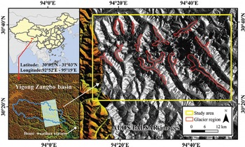
Fig. 1. Location of the Yigong Zangbo basin and the study glaciers.

The YZB has a warm, humid climate, which is determined by strong seasonal variation of precipitation. The mean annual precipitation is 958 mm, with peak precipitation during the India monsoon season between May and September, when it accounts for 74.9% of the annual total according to records from the nearest weather station, Bomi (Fig. 1). The airflow from the Indian Ocean is directed northward along the Yarlung Zangbo river valley and is hindered by the Nyainqêntanglha mountain. Precipitation increases with altitude in the southern slope of the mountain; however, it decreases in the northern slope because of its opposite aspect to the movement of the Indian Ocean airflow. The mean annual air temperature is ∼8.8°C, with highest and lowest mean monthly temperatures of 17.2°C and −1.7°C respectively.

The Indian monsoons, together with the massive topographic landform, cause climatic effects on the distribution of existing glaciers. There are 1724 glaciers in the YZB, all of which are of the temperate or oceanic type because they are affected by warm and humid airflow from the Indian Ocean (Reference Shi and XieShi and Xie, 1964), with the total glacial area and volume of 3910 km² and 444 km³ respectively (Reference YaoYao and others, 2010). The glaciers in the YZB serve the important function of providing water storage and supply for agriculture and economic activities in the lower reaches of the Brahmaputra River.

Dataset

To generate a glacier flow pattern, we needed two SAR images from repeat orbits and an associated digital elevation model (DEM) from the same area. ALOS was launched by the Japanese Aerospace Exploration Agency (JAXA) in January 2006, loaded with three sensors: the Panchromatic Remote-sensing Instrument for Stereo Mapping (PRISM), Advanced Visible and Near Infrared Radiometer type 2 (AVNIR-2) and PALSAR. The L-band PALSAR provides higher performance than the Japanese Earth Resources Satellite 1 (JERS-1) SAR. The PALSAR sensor has a beam with an adjustable elevation and a ScanSAR mode. L-band (wavelength λ = 23.5 cm) SAR can complement existing applications based on C-band (λ = 5.6 cm) data (Reference Strozzi, Kouraev, Wiesmann, Wegmüller, Sharov and WernerStrozzi and others, 2008). It was found in earlier studies that L-band SAR imagery is more suitable for measuring glacier velocity using a feature-tracking method than the C-band imagery, and the HH polarization mode is superior to other polarization modes (Reference JiangJiang and others, 2012). Therefore, for this study, two ALOS/PALSAR orbits, acquired on 3 July and 18 August 2007 (Table 1) and covering the study area (Fig. 1) with HH polarization, were used to estimate the glacier surface velocity. All the images consist of ascending orbit and Single-Look Complex (SLC) data. The data pairs employed in SRFT have a 46 day acquisition interval between images. A total of 12 glaciers are covered by the ALOS/PALSAR images in the basin. We coded the glaciers as Nos. 1–12 because most of them have no published names. Six of the glaciers (Nos. 1–6) are located on the northern slope of the Kona Kangri ridge and the other six glaciers (Nos. 7–12) are located on the southern slope (Fig. 6 further below).

Table 1. ALOS/PALSAR data used for feature-tracking processing

The Shuttle Radar Topography Mission (SRTM) DEM data (version 4) were also downloaded from the website http:// srtm.csi.cgiar.org/ and used to geocode the images and derive the altitude, slope and aspect of the glacier surface. These data have a nominal resolution of 90 m × 90 m and are already hole-filled (Reference Reuter, Nelson and JarvisReuter and others, 2007). All the image products were orthorectified using the SRTM DEM, with the Universal Traverse Mercator (UTM) map projection.

Methods

The flow velocities are derived from sequential satellite imagery using SRFT. The SRFT is implemented by calculating the offsets between two SAR images using offset tracking procedures. The intensity tracking method, also known as the maximum cross-correlation optimization procedure, is used to estimate the slant-range and azimuth registration offset fields of each pair of SAR images. Intensity tracking and coherence tracking are generally used for this purpose. In this approach, prominent surface features that are identifiable on two co-registered images, such as crevasses, rifts or edges that move with the ice, are used to determine the displacement and velocity. The SRFT involves several steps, which are briefly described in the following.

Maximum intensity cross-correlation

Using the SLC images, we estimated the range and azimuth offsets to sub-pixel precision and accurately co-registered the images. We compensated for the residual registration offsets by using a linear transformation based on geomorphological features (e.g. nunataks). This step was performed visually by matching the pixels and such features in ice-free fixed areas.

The image correlation method detects similarities in a pair of co-registered images by examining a matched point between the feature window of the reference (master) image (W_M) and that of the search (slave) image (W_S) (Fig. 2). The centre position of W_M is denoted by P_M, and that of W_S is denoted by P_S. The window with the highest correlation coefficient within the search area is taken to be the most similar window and used to calculate the flow velocity. The search area must be sufficiently large to ensure that the largest possible displacement is included. A larger search window (area-wise) will generally yield a higher matching accuracy, although the offset procedure will require a longer processing time. We experimented with the window size to obtain an optimal balance between the glacier velocity precision and processing time. We set the window size to 64 × 192 pixels and the search step length to 12 × 36 pixels based on several comparison experiments (Reference Strozzi, Wiesmann, Sharov, Kouraev, Wegmüller and WernerStrozzi and others, 2006).

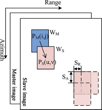
Fig. 2. Schematic diagram illustrating the image correlation method.

In the search procedure, the feature window (with an azimuthal size of A pixels and a range size of R pixels, where A ≠ R) is fixed in the master image and tracked within the larger slave image by shifting the central position, P, of the window (Fig. 2). The match between the two feature windows is a function of the range displacement, v-j, and azimuthal displacement, u-i. In each search, the correlation coefficient r is calculated using Eqn (1) below, and the location, P_S ^* where r is maximized is recorded. The feature window in the master and slave images can be regarded as matched at this location, and P_M in the master image is moved to P_S ^* in the slave image. At this point, the displacement is the distance between P_M and P_S ^*, and the orientation is the direction from P_M to P_S ^*. Subsequently, W_M is moved based on the step lengths, S_R and S_A, and the next displacement is calculated until all the matched feature windows are identified. The normalized correlation coefficient (ranging from −1 to 1) between the master and slave feature windows at the centre location is given by

(1)

where x(i, j) and y(i, j) are the intensity values at range location, i of the master image and azimuth location, j of the slave image respectively, and and are the average intensity values of the entire master and slave feature windows respectively.

The displacement orientation conversion

In this study, the horizontal offsets in the radar geometry were extracted from the data pairs, and the obtained range and azimuth offsets were used to calculate the direction of the glacier motion. To calculate the glacier velocity, the displacement orientation in the SAR geometric coordinate system must be converted to a UTM map projection using (Fig. 3):

(2)

where α _V−UTM is the angle of v in the UTM map projection coordinate system (measured clockwise from the north axis), α _Orbit−UTM is the angle in the azimuthal direction (measured clockwise from the north axis), α _V−SAR is the speed orientation in the SAR geometric coordination system (measured clockwise from the opposite azimuthal direction) and α _{Orbit−Equator} is the oblique angle of the orbit, i.e. the angle in the azimuthal direction measured anticlockwise from the equator. For the ALOS/PALSAR data, α _{Orbit−Equator} is equal to 98.16°.

Fig. 3. The displacement orientation conversion from SAR geometric coordination system to UTM map projection.

Three-dimensional velocity calculation

The displacement D _2D obtained from the SRFT is projected onto a two-dimensional (2-D) horizontal plane (Fig. 4). The three-dimensional (3-D) velocity calculation is based on two hypotheses. The first is that the 2-D glacial surface velocity derived using the SRFT method is the horizontal projection of the 3-D velocity, and the second is that the direction of the 3-D velocity at a certain point is parallel to the topographic slope of the 2-D velocity at the same point. The 3-D displacement D _3D, which is the actual displacement of the glacier surface, can then be converted using the DEM and computed as

(3)

where D _2D is the displacement of point P in the 2-D plane, D _3D is the displacement in 3-D space, and θ is the slope angle of point P along the D _2D direction. It is important to note that the value of θ is not simply the value calculated from the traditional DEM slope because the slope value calculated from the DEM considers the steepest gradient. However, the displacement based on the SRFT is not necessarily oriented along the steepest gradient and must be determined to the projection direction in the 2-D plane of the glacier velocity.

Fig. 4. Horizontal velocity and actual velocity of the glacier surface.

Finally, the glacier velocity can be calculated as

(4)

where V _a is the annual mean velocity (m a⁻¹) and D _3D is the displacement in 3-D space during the time interval between the acquisition of the two images (46 days for ALOS/PALSAR imagery).

Error analysis

The largest sources of error in the feature-tracking-based velocities are the image geolocation, co-registration and feature-tracking method errors (Reference Wuite, Jezek, Wu, Farness and CarandeWuite and others, 2009). In order to evaluate the errors, we randomly selected 200 fixed points, which were often identified with well-defined SAR surface features such as naked rocks or ridges by spanning the SAR images around the glacier area and seeking the best-correlated templates using the same size adopted to extract the ice velocity field. Table 2 shows the maximum, minimum and mean errors along different aspects are 12.03, 0.39 and 4.03 m a⁻¹ respectively. Figure 5 further indicates that there is no evident relationship between error and aspect, range or azimuth direction.

Table 2. Errors (m a^–1) of aspect, azimuth and range directions

Fig. 5. Error distribution and analysis: (a) aspect; (b) azimuth direction; (c) range direction.

After the SRFT processing, a final filtering was performed to eliminate the bad vectors. The filter was based on the minimum and maximum modulus thresholds, exclusion of isolated vectors and omission of vectors that differ significantly in modulus or direction from the average vector at a given radius.

Results

Three-dimensional glacier flow patterns

The available SAR image pairs (Table 1) were successfully used to estimate the surface velocity patterns in the YZB. Here we investigate the potential of the SRFT method to estimate the glacier flow. The glacier boundaries were derived from the Global Land Ice Measurements from Space (GLIMS) database (http://www.glims.org/) and were modified by visual interpretation of the SAR images. To aid in their presentation and interpretation, the flow patterns were superimposed onto ALOS/PALSAR intensity images in Figure 6. Figure 6 provides a map of the magnitude of the 3-D flow velocity vectors, and the arrows in Figure 10 denote the magnitude and direction projection of the 3-D flow velocity vectors in 2-D plane. Many topographic features of the glaciers are evident from the DEMs of both Figures 1 and 6; these features confirm certain basic lateral patterns of the motion of the valley glaciers and provide a better understanding of the glacier motion. Mountains are present on both sides of the glaciers and limit the movement of the glaciers in a particular direction. Immediately adjacent to the side-walls of the valley glaciers, the ice is nearly motionless owing to lateral and bottom friction. Far from the side-walls, the flow velocity increases to a maximum around the central flowlines. The glacier surface velocity distributions throughout the YZB display strong spatial variations with changes in elevation. There are six glaciers (Nos. 1–6) in the north slope and six glaciers (Nos. 7–12) in the south slope. Due to the constraint of valley geometry and terrain complexity, the six glaciers in the north slope show different flow directions, with glaciers Nos. 1–4 flowing north, No. 5 northwest and No. 6 northeast. By contrast, six glaciers in the south slope all flow southeast. Along the central flowlines of the glaciers, there are multiple local maxima or minima, indicating that the velocity of the glacier flow down-valley is not constant (Fig. 7). The mean velocities of the 12 glaciers fall between 15 and 206 m a⁻¹ (Table 3), with Glacier No. 5a showing a maximum velocity of 423 m a⁻¹. Because all the studied glaciers are oceanic-type, their velocities are generally greater than those of continental-type glaciers which are affected by continental-type climate (Reference Huang and SunHuang and Sun, 1982).

Fig. 6. Flow velocity of glaciers in the YZB.

Table 3. Flow velocity of glaciers in the YZB

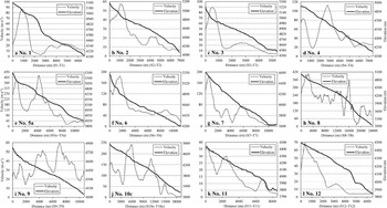
Fig. 7. Profiles of glacier flow velocity and elevation.

Along-axis glacier flow patterns

To provide a more quantitative analysis, the velocity profiles of the glaciers along the approximate central flowlines (Fig. 6 for positions) are shown in Figure 7, which also includes glacier surface elevations. The velocity values (m a⁻¹) and distance (m) are shown along the central flowlines, starting from the accumulation zone (starting point) down to the terminal zone of the glaciers. Although the glacier surface elevation continually decreases down-valley, the derived velocity profiles display significant variations along the central flowlines of the glaciers. The 12 glaciers behave similarly in terms of their spatial variation. Most of the glaciers have high velocities in their upper sections and low velocities in their lower sections, and in general, a larger glacier size corresponds to a higher velocity.

Glacier area and length, derived from visual interpretation of the ALOS/PALSAR images with the support of the GLIMS database, are shown in Table 3. The velocity displays a positive relationship with the glacier area and length (Figs 8 and 9). This result is consistent with the conclusions of Reference Huang and SunHuang and Sun (1982). In the upper section of Glacier No. 8, the longest of the glaciers examined in this study, the velocity was ∼402 m a⁻¹ at an elevation of 5012 m and then increased to a maximum of ∼405 m a⁻¹ at a distance of 2395 m and elevation of ∼4795 m. Between distances of 2395 and 14 300 m, the flow gradually decreased to a local minimum of ∼173 m a⁻¹;the velocity then fluctuated down-glacier and reached another local maximum of 273 m a⁻¹. The glacier motion in the lower section is of great interest due to its large-scale spatial variations. Beyond a distance of 14 300 m, the velocity abruptly decreased to a local minimum of ∼80 m a⁻¹, and the flow subsequently increased suddenly and reached a local maximum of ∼359 m a⁻¹ at a distance of 16 044 m and elevation of ∼3929 m. Below this elevation, the flow decreased abruptly to a minimum of ∼12 m a⁻¹. The velocity profile pattern exhibited small-scale spatial variations with a further decrease in elevation towards the glacier terminus, and the flow velocity reached 159 m a⁻¹ at a distance of 20 793 m and elevation of ∼3305 m. Subsequently, the velocity decreased gradually to 73 m a⁻¹ at the glacier terminus. The flow field of Glacier No. 8 is shown in Figure 10, and the uppermost layer includes the glacier flow vectors (indicated as arrows). As shown in Figure 10, the spatial pattern of the derived velocities and directions appears to be consistent with the glacial and topographic features.

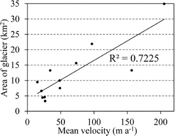
Fig. 8. Relationship between mean flow velocity and glacier area.

Fig. 9. Relationship between mean flow velocity and glacier length.

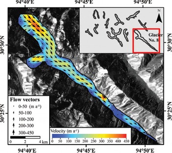
Fig. 10. Flow velocity and field of Glacier No. 8.

Discussion

The equilibrium-line altitude (ELA) of a glacier is very sensitive to climate change. The ELA is tightly correlated with solid precipitation and air temperature (Reference Cui and WangCui and Wang, 2013). According to the theory of glacier kinematics, glacial surface velocity reaches the maximum near the ELA (Reference JiangJiang and others, 2012). Therefore, the elevation where maximum glacial surface velocity occurs will, to some extent, indicate the location of the ELA. We can infer the locations of the ELA (black dashed curves in Fig. 6) from the maximum velocity in the central flowline of each glacier. Figure 6 and Table 3 indicated that ELA locations of all glaciers are between 4300 and 5200 m, identical to results from other studies (Reference Korup and MontgomeryKorup and Montgomery, 2008; Reference YaoYao and others, 2010). Table 3 indicates that the ELAs on the north slope are higher than on the south slope, and all are higher than 4600 m. The highest ELA is ∼5100 m on Glacier No. 1. The ELAs on the south slope are lower than 4600 m except for Glacier No. 8, and the lowest ELA is ∼4330 m on Glacier No. 9. We can understand the mass balance if we know the interannual ELA change: an upward-moving ELA indicates negative glacial mass balance, and the converse.

Little is known regarding the behaviour of the YZB glaciers, and few field studies have been performed in this glacial area owing to the harsh weather and difficult topographic conditions. There are no ground measurements of glacier flow velocity in the YZB, and glacier movement studies based on remote-sensing methods have not previously been reported. However, ground measurements of the glacier flow velocity on Hengduan mountain can account for the results presented in this paper. Hengduan mountain, which contains oceanic-type glaciers and is adjacent to the YZB, is also located in the eastern Tibetan Plateau and is similarly impacted by the Indian Ocean monsoon. Because the ALOS/PALSAR images were acquired on 3 July and 18 August of 2007, the annual mean velocity was calculated using summer data only. However, the glacier velocities during the summer are typically greater than those during the other seasons in western China (Reference Jing, Zhou and LiuJing and others, 2010). Therefore, the annual mean velocity calculated in this paper for the YZB glaciers is slightly greater than the values reported for Hailuogou glacier (Reference Xie and LiuXie and Liu, 2009).

Reference JiangJiang and others (2012) analysed the surface velocities of Yengisogat glacier, Karakoram, Tibetan Plateau, using ALOS/PALSAR data from 2007 to 2009 using the feature-tracking method. Their results indicated that the velocities along the central flowlines of the various tributaries ranged between 10 and 400 m a⁻¹ during the summer. These significant variations in derived velocity are similar to those found in this study and demonstrate that our results are reasonable.

Glacier retreat is pronounced in the YZB (Reference YaoYao and others, 2012). Glaciers in the YZB are expected to be especially sensitive to present-day atmospheric warming. Glacier dynamics and variations are believed primarily to reflect the monsoon dynamics (Reference YaoYao and others, 2012). As glacier size decreases, glacier velocity also gradually decreases; this phenomenon is significant in the YZB (Reference Jing, Zhou and LiuJing and others, 2010). This trend is observed not only in the YZB but also in most other glaciated areas in China. On the whole, glacier velocities in the Tien Shan have decreased slowly, there has been a very small decrease in glacier movement in the Himalaya since 1990 and there has been a significant decrease in glacier velocity on Hengduan mountain (Reference Jing, Zhou and LiuJing and others, 2010), which is similar to that observed in the YZB. In addition to the glacier size, the topographic slope, basal rock and other factors all play important roles in the glacier velocity. There is an urgent need for a comprehensive investigation of the surface, internal and basal movement of glaciers in the near future.

Owing to their spatial and temporal detail, SAR images are likely to become an increasingly important glaciological tool in both the synoptic analysis of ice surface velocities and identification and explanation of ice motion events. The SRFT methodology represents a useful tool for obtaining glacier velocity measurements using optical or microwave imagery, especially under difficult geographical conditions (Reference KääbKääb, 2005; Reference JiangJiang and others, 2012; Reference Scherler and StreckerScherler and Strecher, 2012). SRFT can be used to obtain glacier velocity fields not only over a large scale but also with a high spatio-temporal resolution. However, the results should be validated using site measurements. Field measurement records of glaciers in the Tibetan Plateau are rare, which hinders research on glacier motion even when remote-sensing methods are used. The integration of remote-sensing and continuous in situ measurements of representative glaciers in the Tibetan Plateau is therefore highly recommended for future glaciological research in the context of climate warming.

Conclusion

This study provides ice-velocity mapping for several glaciers in the YZB using the feature-tracking methods, based on ALOS/PALSAR images acquired on 3 July and 18 August 2007. The results demonstrate that SAR feature tracking is a suitable method for retrieving glacier surface flow velocities, especially in cloud- and snow-covered areas where visible optical imagery is problematic. The observation of flow maxima as well as several local maxima and minima at consistent locations suggests that valley geometry and local topography affect the overall spatial pattern of the flow velocities. A large set of SAR data is required to detect seasonal changes in the glacier motion patterns and to estimate the mass balance, while routine monitoring of valley glacier movement in the YZB is needed to provide such valuable information under current climate-change scenarios.