


1. Introduction
Arctic sea ice, on track towards a thinner seasonal ice cover (e.g. Reference Kwok, Cunningham, Wensnahan, Rigor, Zwally and YiKwok and others, 2009), is an important component of the Earth system. Sea ice is known to influence, among others, global climate and oceanic circulation (Reference AagaardAagaard, 1981; Reference Curry, Schramm and EbertCurry and others, 1995), major biogeochemical cycles (e.g. Reference Thomas, Papadimitriou, Michel, Thomas and DieckmannThomas and others, 2010) and the transport and fate of contaminants (e.g. Reference Pfirman, Eicken, Bauch and WeeksPfirman and others, 1995). An understanding of the roles played by Arctic sea ice in the Earth system requires a good knowledge of its physical (temperature and bulk salinity) and textural (size, shape and orientation of ice crystals) properties. The conventional approach is to consider the relationships between sea-ice temperature and bulk salinity and the fraction volume and salinity of the brine entrapped in the ice (Reference Cox and WeeksCox and Weeks, 1983). As liquid (brine) and solid (pure ice) phases have very different attributes, most sea-ice properties are influenced by the amount, size and shape distribution of brine in the ice (referred to as ice microstructure). This is the case, for example, for the strength and mechanical behavior of the ice (Reference Timco and FrederkingTimco and Frederking, 1990) and shortwave radiation scattering in the ice (Reference Perovich, Roesler and PegauPerovich and others, 1998). The influence on sea-ice permeability is probably the most remarkable (Reference Freitag and EickenFreitag and Eicken, 2003). Above a critical threshold in brine volume fraction, brine inclusions become interconnected and the ice is considered permeable to fluid transport (Reference Eide and MartinEide and Martin, 1975; Reference Golden, Ackley and LytleGolden and others, 1998). The control exerted by permeability on the mobility and exchanges at the ocean–ice–atmosphere interface of key biogeochemical variables is highlighted in many studies. This is the case, for example, for algal biomass (Reference Krembs, Gradinger and SpindlerKrembs and others, 2000) and nutrients (Reference Fritsen, Lytle, Ackley and SullivanFritsen and others, 1994), for contaminants such as mercury (Reference Chaulk, Stern, Armstrong, Barber and WangChaulk and others, 2011) and for climate active gases such as CO2 (Reference GeilfusGeilfus and others, 2012) and dimethylsulfide (Reference Tison, Brabant, Dumont and StefelsTison and others, 2010). Textural properties provide information on sea-ice formation, growth and decay processes and are therefore also connected to sea-ice halo-thermodynamic evolution. Formation and growth processes define, for example, how scalars (including salts) are initially incorporated in sea ice, as shown for algal biomass by Reference Ackley and SullivanAckley and Sullivan (1994). For all these reasons, detailed physical and textural analyses constitute the basis for many other investigations of the sea-ice system.
Numerous investigations of the sea-ice system were conducted during the International Polar Year Circumpolar Flaw Lead (IPY-CFL) system study in the southern Beaufort Sea–Amundsen Gulf, Canadian Arctic (Fig. 1), aboard the icebreaker CCGS Amundsen from 18 October 2007 until 7 August 2008. Over 350 participants, organized in 12 teams (for details see Reference BarberBarber and others, 2010), tried to answer a wide range of key scientific questions related to the different roles played by Arctic sea ice in the Earth system. The initial objective of the present study was to provide a common interpretative framework of physical (temperature and bulk salinity) and textural properties to the IPY-CFL community and especially for investigations based on ice coring, which is often carried out for a wide range of multidisciplinary projects (e.g. Reference LewisLewis and others, 2011). The same framework should also be of some interest for future experiments in the Amundsen Gulf. We therefore measured sea-ice temperature and bulk salinity from ice cores collected throughout the sampling season. We also regularly made textural analysis based on thin-section pictures. We ended up with a large dataset covering a complete cycle from growth to the start of melt (i.e. 28 November 2007 to 18 June 2008).
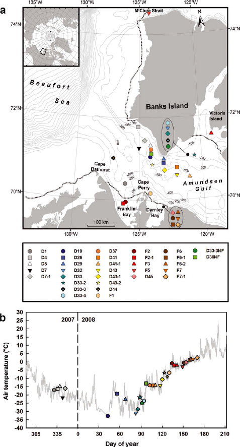
Fig. 1. (a) Map of the study area showing the bathymetry and the location of the sampling stations. The dotted lines indicate the extent of fast ice on 5 May 2008. Data for fast-ice extent delimitation were obtained from the Canadian Ice Service sea-ice charts. (b) Air temperature recorded during the IPY-CFL study. The sampling stations icons are plotted on a temperature series of air temperature measured with a Rotronics MP 101A temperature sensor located at ~18 m above the ice surface with a resolution of 0.1°C and an accuracy of ±0.3°C.
Measurements of sea-ice temperature and bulk salinity extending over such a long time period are very scarce. Field observations are usually limited to the spring and summer seasons due to technical difficulties inherent to winter sampling. Hence, our dataset represented a unique opportunity to investigate the halo-thermodynamic evolution of sea ice over a long period. The annual cycle of sea-ice temperature has been well described by Reference Perovich and ElderPerovich and Elder (2001). Sea-ice temperatures in first-year Arctic sea ice are generally driven by the surface heat balance and buffered by the snow cover, the oceanic heat flux typically being small in most regions of the Arctic (Reference Steele, Flato, Lewis, Jones, Lemke, Prowse and WadhamsSteele and Flato, 2000). The annual cycle of sea-ice bulk salinity is governed by sea-ice desalination processes. Sea-ice desalination is critical as it directly influences oceanic circulation (e.g. Reference AagaardAagaard, 1981). Some early time series of sea-ice bulk salinity showed salinity profiles typically C-shaped in winter cores and Z-shaped when surface melting occurs (Reference Malmgren and SverdrupMalmgren, 1927). In another time-series study, Reference Nakawo and SinhaNakawo and Sinha (1981) investigated the effect of growth rate on salinity. They showed that from a few days after ice formation until warming in spring the salinity of an ice layer remains stable. Reference UntersteinerUntersteiner (1968) suggested several potential sea-ice desalination mechanisms. Two of these mechanisms (brine diffusion and brine expulsion) only lead to salt redistribution within sea ice but do not contribute to any measurable sea-ice desalination (Reference Notz and WorsterNotz and Worster, 2009). On the contrary, it is generally agreed that flushing results in an important and net salt loss during the melt season (Reference Eicken, Grenfell, Perovich, Richter-Menge and FreyEicken and others, 2004; Reference Notz and WorsterNotz and Worster, 2009). The hydraulic head created by the snow and surface ice meltwater flushes downwards the existing brine network. Before the melt season and during ice growth, it was generally assumed that salt loss was governed by segregation of salts at the ice–ocean interface (Reference Cox and WeeksCox and Weeks, 1988). Segregation of salts was considered to be a function of ice growth rate, with higher salinities obtained at higher growth rates. In the past two decades, several studies suggested that the salt loss observed during ice growth and warming was uniquely the result of gravity drainage (e.g. Reference Wettlaufer, Worster and HuppertWettlaufer and others, 1997; Reference Vancoppenolle, Fichefet and BitzVancoppenolle and others, 2006; Reference Notz and WorsterNotz and Worster, 2009).
Gravity drainage is the convective overturning of brine in connected brine inclusions (Reference Cox and WeeksCox and Weeks, 1975; Reference Notz and WorsterNotz and Worster, 2008). With gravity drainage, the net desalination is caused by the salinity difference between the brine leaving the ice and the brine entering the ice. Gravity drainage is governed by the ice thickness, the permeability and the brine density gradient (Reference Wettlaufer, Worster and HuppertWettlaufer and others, 1997, Reference Wettlaufer, Worster and Huppert2000). These relationships have been approached analytically in the mushy-layer theory (Reference WorsterWorster, 1992; Reference Wettlaufer, Worster and HuppertWettlaufer and others, 1997) using a porous-medium Rayleigh number. For gravity drainage to occur, the Rayleigh number must exceed a critical value. Based on experimental studies, it was estimated to be typically 10 (Reference Wettlaufer, Worster and HuppertWettlaufer and others, 1997; Reference Notz and WorsterNotz and Worster, 2009). For a given ice depth, gravity drainage only occurs once the buoyancy forces due to the vertical brine density gradient expressed in the numerator of the Rayleigh number overcome dissipation (the product between dynamic viscosity and thermal diffusivity of the brine), as expressed by the denominator. In growing cold ice, gravity drainage is limited to the permeable ice layer at the interface with the ocean, which gives rise to a quasi-steady-state salinity. In warming permeable ice, full-depth gravity drainage can develop, which results in a net desalination of the ice cover.
The Rayleigh number has had some success as a proxy of sea-ice desalination in laboratory experiments. However, it has rarely been applied to field measurements (Reference Wettlaufer, Worster and HuppertWettlaufer and others, 2000; Reference Notz and WorsterNotz and Worster, 2008; Reference Gough, Mahoney, Langhorne, Williams and HaskellGough and others, 2012) and certainly not over a complete cycle from growth to start of melt. The large dataset presented in this study provided an opportunity to achieve this. We therefore apply the evolution of the measured mean bulk ice salinity from November 2007 until June 2008 to the evolution of both calculated brine volume fraction and Rayleigh number. It should be acknowledged here that this study was not initially designed as a real time-series study. Hence our dataset also integrates spatial variability, which we also discuss.
Finally, we provide a regional analysis of the sea-ice formation and deformation processes based on textural analysis. The Amundsen Gulf is an oceanic area of particular interest since it is characterized by the development of polynya and flaw leads (Reference Barber, Massom, Smith and BarberBarber and Massom, 2007). Expected to increase in number and to expand in size and duration, such areas could also represent a glimpse of the future sea-ice conditions in the Arctic.
2. Materials and Methods
2.1. Study area and sampling strategy
The IPY-CFL study was conducted aboard CCGS Amundsen in the southern Beaufort Sea–Amundsen Gulf area between 18 October 2007 and 7 August 2008 (Fig. 1). The region’s sea-ice climatology has recently been described by Reference Galley, Key, Barber, Hwang and EhnGalley and others (2008) over 1980–2004. Sea ice in the Amundsen Gulf generally starts to form in October in shallow areas along the coast as fast ice, while a drift-ice regime with small leads dominates offshore. In some years, fast ice covers the entire Amundsen Gulf over winter and early spring. Interaction between the fast-ice edge that develops between Cape Perry and Banks Island and the perennial mobile pack ice that rotates with the Beaufort Gyre is responsible for the development of the flaw lead (Reference Proshutinsky, Bourke and McLaughlinProshutinsky and others, 2002; Reference Barber and HanesiakBarber and Hanesiak, 2004). Break-up in the Amundsen Gulf usually occurs in early June and creates the feature known as the Cape Bathurst polynya.
A description of sea-ice dynamics in the Amundsen Gulf in 2007 and 2008 is available from Reference BarberBarber and others (2010). Sea ice was highly mobile in 2007 and 2008. In 2007, sea-ice formation started around the third week of September, and by 26 October freeze-up was complete (Reference BarberBarber and others, 2010). Strong easterly winds kept the sea ice mobile throughout much of the winter season. Fast ice remained restricted to nearshore locations while a sea-ice regime characterized by drifting floes interspersed with small short-lasting leads continued to dominate until ice break-up in the first week of May 2008 (Reference BarberBarber and others, 2010).
Samples analyzed in this study were collected during the IPY-CFL study between 28 November 2007 and 18 June 2008 in approximately area 69–75° N, 119–127° W (Fig. 1). The IPY-CFL was a multidisciplinary study. Sampling site selection was aimed to satisfy a multitude of research objectives (Reference BarberBarber and others, 2010). The initial plan was to establish a semi-permanent ice camp along a fast-ice edge that usually forms between Banks Island and Cape Perry (Fig. 1). However, since sea ice was highly mobile in 2007 and 2008 the ship was constantly repositioned for safety and logistical reasons. This resulted in a geographic dispersion of the sampling sites across the Amundsen Gulf. The ship repositioned in numerous drift-ice sites south of Banks Island (Fig. 1) over a period between the end of November and the first week of May and associated ice break-up. Thereafter, the ship moved to nearshore fast-ice sites primarily located in two sheltered bays (Franklin and Darnley Bays) (Fig. 1). One fast-ice site in the mouth of M’Clure Strait and one on the west coast of Victoria Island were also visited (Fig. 1).
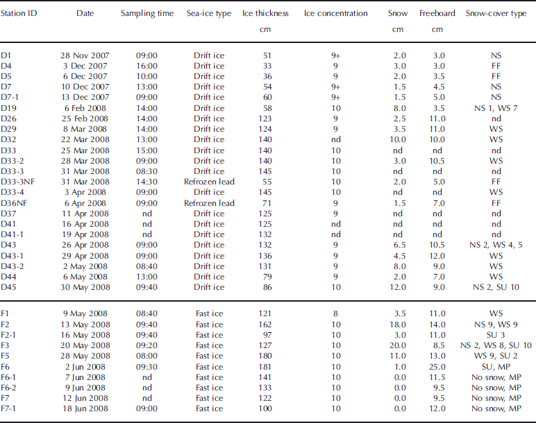
Samples from 21 of the sites (15 drift-ice and 6 fast-ice sites) visited by the ship are analyzed here. The time spent at each of these sites varied between a few hours and 22 days. Generally, one ice floe was sampled at each site during 1 day. However, for some sites where the ship stayed for a few days, the IPY-CFL teams collected samples on multiple days and each day on a different ice floe. In this study, each of these sampling days is referred to as a station. In total, we report measurements from 33 stations (23 drift-ice and 10 fast-ice stations) (Table 1). The stations were named by a letter (D for drift ice, F for fast ice), a number (ID of the site) and a hyphen followed by a number if there was more than one station per site. On two occasions, NF (newly formed) letters were added to the name of the station to designate sampling of sea ice recently formed in a refrozen lead. The location of the stations is shown in Figure 1. Also shown is the extent of fast ice on 5 May 2008 drawn from the Canadian Ice Service sea-ice charts. On average, sampling occurred every 5 days over the study period. However, sampling was suspended between 13 December 2007 and 6 February 2008 since no member of our research team was aboard the ship at that time.
Table 1. General ice and surface conditions at the sampling stations. Time is local time (GMT-7). Ice concentrations are given in tenths. The horizontal line separates drift-ice stations from fast-ice stations. NS: new snow; FF: frost flowers; WS: wind slabs; SU: superimposed ice; MP: melt ponds; nd: not determined
2.2. Sampling and measurements
Sampling always started with ice floe selection. The criteria used to select a floe included floe size (large floes of a few hundred meters or greater were preferred), and a minimum distance from pressure ridges (>500 m) was enforced. An area dedicated to the ice coring was delimitated on the ice floe upwind of the ship and access to the area limited to the team members to ensure pristine conditions. Within this area, a small work sub-area (~5 m × 5 m) with homogeneous surface conditions was selected to limit spatial variability. On a few occasions, an ice cage lowered from the ship was used for sampling. This occurred over thin ice in November and December and when the ship was navigating in refrozen leads later in the field season (stations D33-3NF and D36NF).
Once on the ice floe, snow-cover type and conditions (wetness, hardness and grain size) were characterized by visual observations using the terminology of Reference MassomMassom and others (2001) and Reference Sturm, Holmgren and PerovichSturm and others (2002). These are reported in Table 1. Snow thickness was measured with a ruler. A maximum of ten sea-ice cores were then collected using an electropolished stainless-steel corer (Lichtert Industry®, Belgium) (ID = 7 cm) for various biogeochemical analyses. Only two of these cores from each station were used in this study. The first sea-ice core was dedicated to sea-ice temperature, bulk salinity and water stable-isotope (δ18O) measurements, while the second was dedicated to sea-ice texture determination. The distance between the two sea-ice cores was always <20 cm. Core lengths and freeboard were measured with a ruler after extraction. These are also reported in Table 1.
Sea-ice temperature, T (°C), was measured in situ on the first core extracted at each station. The delay between core extraction and the beginning of the measurement was always very short (<60 s). A fast-response handheld portable digital thermometer equipped with a calibrated probe (TESTO® 720) was used. The probe was inserted in 2 mm diameter holes drilled to the center of the core at 5 cm intervals. In case the end of a 5 cm interval corresponded to a crack in the core, the measurement was made a few centimeters further. The precision of the probe was ±0.1°C with an accuracy of ±0.2°C. The drilling process may have impacted both the accuracy and precision of the sea-ice temperature measurements, but it is doubtful that the effect will have been large given the high heat capacity of sea ice (Reference UntersteinerUntersteiner, 1961).
The same ice core was then immediately cut into sections with a stainless-steel saw using the same vertical resolution as for sea-ice temperature. The whole process typically took 5–10 min depending on the core length. Ice-core sections were stored in sealed plastic containers and melted at room temperature aboard the ship. Sea-ice bulk salinity, S i, of each melted core section was determined through conductivity using a Thermo-Orion® WP-84TPS meter (accuracy of ±0.1‰). Salinity data are reported using the practical salinity scale.
Water aliquots (10 mL) were also collected in no-headspace vials from the melted core sections for water stable-isotope (δ18O) measurements. Snow was always carefully scraped off the surface of the ice cores collected, to avoid snow contamination of the samples. Aliquots were analyzed at the G.G. Hatch Isotope Laboratories, University of Ottawa, using a Gasbench + DeltaPlus XP isotope ratio mass spectrometer (ThermoFinnigan®, Germany) and the conventional water–CO2 equilibration method (accuracy with respect to Vienna Standard Mean Ocean Water (VSMOW) was ±0.15‰). Water stable-isotope (δ18O) data are reported as per mil deviation of the 18O/16O ratio of the CO2 equilibrated with the water samples relative to VSMOW:
The second ice core collected was stored in an insulated box filled with ice packs precooled to −30°C and brought back to the ship. The core was stored horizontally at −26°C until processing as suggested by Reference Eicken, Lange and DieckmannEicken and others (1991). Vertical sections of the ice core were attached to glass plates and planed down to 0.6–0.8 mm using a microtome (Leica® SM2400). The thin sections obtained were installed on a light table equipped with cross-polarized sheets, and pictures were taken with macro setting activated on the camera (Nikon® Coolpix S200, 7.1 megapixels) following the standard procedure presented by Reference LangwayLangway (1958). The size, shape and orientation of the crystals were used to discriminate between the different textural types. Since the differences in crystal properties between the different ice layers were easily identifiable on the pictures, c-axis orientation measurements with a universal stage were not made.
Air temperature was recorded on the ship deck by a Rotronics MP 101A temperature sensor located at ~18 m above the ice surface. The sensor had a resolution of 0.1°C and an accuracy of ±0.3°C. Geographical coordinates and ice conditions (ice type and concentration) of the sampling sites were available from the ship logbook and from the Canadian Ice Service sea-ice charts.
3. Results
3.1. General ice properties and surface conditions
The evolution of the air temperature during the sampling season as recorded by the temperature sensor located on the ship’s deck is shown in Figure 1. An icon was then added to this temporal series at the corresponding sampling date of each station. General ice properties (ice type, thickness and concentration) and snow-cover properties (snow type, thickness and freeboard) are reported in Table 1. All stations sampled were first-year ice and the freeboard was always positive.
The first sampling period occurred between 28 November 2007 (day 331) and 13 December 2007 (day 347) in the Amundsen Gulf between Cape Perry and Banks Island (Fig. 1). Air temperature decreased from November to December with the progression towards winter (ranging between −25°C and −15°C). Five stations were sampled during this period (D1 to D7-1). All stations consisted of thin drift ice (30–60 cm thick), and the ice concentrations were always high (9 to 9+ tenths). The snow cover was typically thin (1.5–3.0 cm) and consisted of new snow. Frost flowers were observed at stations D4 and D5.
Sampling was then suspended for roughly a month and a half due to a lack of team members aboard the ship. Sampling resumed on 6 February 2008 and was continuous until 18 June 2008. From 6 February 2008 (day 37) until 3 April 2008 (day 94), the air temperature recorded at the stations remained low (<−20°C). During this period, eight stations (D19 to D33-4) were sampled in the Amundsen Gulf just south of Banks Island (Fig. 1). Most stations consisted of medium and thick drift ice (58–145 cm thick) and the ice concentrations were always high (9–10 tenths). The snow cover (2.5–10.0 cm) consisted either of a thin wind slab layer (cohesive layer of snow formed when wind deposits snow onto sea ice) or of a thin new snow layer over a thicker wind slab layer. One thinner station (D33-3NF on 31 March 2008, 55 cm thick) was clearly identified by observers as a recently refrozen lead and had frost flowers at its surface.
From 3 April 2008 until the end of the sampling season, the air temperature recorded at the stations rose almost continuously. Between 3 April 2008 (day 91) and ice breakup (first week of May), eight additional drift-ice stations (D36NF to D44) were sampled. These were located in the Amundsen Gulf, just south of Banks Island and north of Cape Bathurst (Fig. 1). The stations consisted of medium and thick ice (71–136 cm thick), and ice concentrations were high (9-10 tenths). Air temperature ranged between −15°C and −5°C. The snow cover varied from a thin wind slab layer (1.5–2.0 cm) on the medium ice to a thicker wind slab layer (4.5–8.0 cm) on the thick ice. One refrozen lead station (D36NF) had relic frost flowers buried in snow at its surface.
After ice break-up, the ship visited fast-ice stations. The extent of fast ice on 5 May 2008 is shown by dashed lines in Figure 1. From 9 May 2008 (day 130) until 28 May 2008 (day 149), five fast-ice stations (F1–F5) were sampled in various locations such as Franklin Bay, the mouth of M’Clure Strait and the west coast of Victoria Island (Fig. 1). The ice cover was thick at all stations (97–180 cm thick), and ice concentrations ranged between 8 and 10 tenths. Air temperature was high, ranging between −5°C and 0°C. Signs of surface melting appeared and 2–10 cm of superimposed ice was observed at stations F2-1 to F5.
Six more stations were sampled in Darnley Bay (Fig. 1) after 30 May 2008 (day 151), corresponding to the air temperature rising above 0°C. The first station (D45 on 30 May 2008) consisted of medium drift ice (86 cm thick) with a 10 cm layer of superimposed ice under 2 cm of new snow. The five remaining stations (F6 to F7-1) were on thick fast ice (100–181 cm thick), with a very thin layer of superimposed ice at station F6 and no snow at all the other stations. Melt ponds were observed at station F6 (2 June 2008) and at subsequent stations until the end of the field season.
3.2. Sea-ice temperature and bulk salinity
Depth profiles of sea-ice temperature (T) and bulk salinity (S i) at each sampling station are provided in Figures 2 and 3. Ice temperature profiles measured during the first sampling period (D1 to D7-1) showed a general linear increase from a cold surface to a warmer ice base held at its melting point. The vertical ice temperature gradient (∂T/∂z) was calculated as the difference between temperatures at the ice surface and base, divided by the ice thickness (a positive value indicating a negative heat flux through the ice). The mean gradient during the first sampling period (28 November 2007 to 13 December 2007) was 17°C m−1. Comparable gradients (averaging 16°C m−1) were observed at stations between D19 (6 February 2008) and D36NF (6 April 2008) although the actual temperature difference across the ice vertically was larger. From station D37 (11 April 2008) until station D44 (6 May 2008), we observed that the gradients slackened (averaging 5°C m−1),corresponding to an increase in surface ice temperature. The last drift-ice station sampled (D45 on 30 May 2008) had a slightly negative gradient (−1°C m−1) in its top 20 cm, while deeper ice was near-isothermal. Sea ice was near-isothermal at all the coldest fast-ice stations (from F1 on 9 May 2008 until F5 on 28 May 2008) with gradients averaging 1°C m−1. Some stations (F2, F2-1 and F5) also had a slightly negative gradient in their surface ice sections. Finally, the warmest fast-ice stations (from F6 on 2 June 2008 until F7-1 on 18 June 2008) were close to melting at all depths.
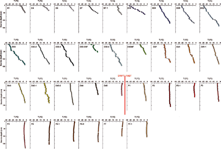
Fig. 2. Vertical profiles of sea-ice temperature (T) at the sampling stations.
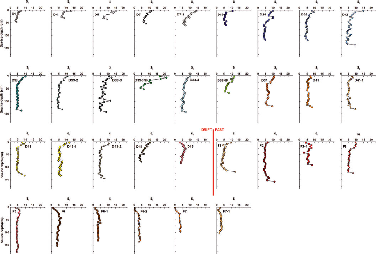
Fig. 3. Vertical profiles of sea-ice bulk salinity (S i) at the sampling stations.
Ice salinity profiles (Fig. 3) were C-shaped from station D1 (28 November 2007) until station D44 (6 May 2008) as typically observed in growing sea ice (e.g. Reference Nakawo and SinhaNakawo and Sinha, 1981; Reference Eicken, Lange and DieckmannEicken and others, 1991). However, the pattern was not always perfectly defined. Some stations had much higher surface ice salinity relative to bottom salinity. These were stations sampled between 3 December 2007 (D4) and 6 February 2008 (D19) as well as station D33-3NF, which corresponded roughly to all the thin-ice stations. The ice salinity profile of the last drift-ice station sampled (D45 on 30 May 2008) transitioned to a ?-shape, as previously described by Reference Eicken, Lange and DieckmannEicken and others (1991). Surface ice became fresher while a bottom maximum in salinity vanished. Fast-ice stations had variable salinity profiles. Stations F1 and F2 had C-shaped profiles, stations F2-1 and F3 reverse S-shaped profiles (Reference Eicken, Lange and DieckmannEicken and others, 1991; Reference EickenEicken, 1992), while ?-shaped profiles were observed at all other stations.
3.3. Sea-ice textural properties and water stable isotope (δ18O)
Samples of ice texture are presented in Figure 4. This selection of stations gives a good overview of the ice surveyed during the IPY-CFL study as it covers most of the sampling season and the different ice types (drift ice/fast ice). We identified five different ice textures (granular, columnar, mixed columnar/granular, platelet and draped platelet) in the thin-section pictures based on descriptions found in the literature (Reference Eicken and LangeEicken and Lange, 1989, Reference Eicken and Lange1991; Reference Jeffries, Weeks, Shaw and MorrisJeffries and others, 1993; Reference Tison, Lorrain, Bouzette, Dini, Bondesan, Stiévenard and JeffriesTison and others, 1998). Granular texture was always orbicular rather than polygonal (Fig. 4a). Some polygonal granular ice, corresponding to superimposed ice, was observed during the study (see Table 1) but systematically scraped off the ice surface before sampling. Hence it could not be detected in the thin-section pictures. Three granular orbicular sub-textures, fine grain sizes (<2 mm across), medium grain sizes (2–5 mm across) and coarse grain sizes (>5 mm across) were observed. Typically, cores had a thin layer of granular orbicular texture underlain by columnar texture (Fig. 4b). On average, granular texture represented 9% (ranging between 0 and 49%) of the total ice thickness and columnar texture 87% (ranging between 50 and 100%). Thin layers of granular texture (1–2 cm) were also occasionally found in interior ice (e.g. D7-1 and D32). Mixed columnar/granular texture (Fig. 4c) was found at five stations (D29, D33-2, D43-1, D45 and F1) and represented 4–17% of the total ice thickness of these stations.

Fig. 4. Sea-ice textural properties for a subset of the sampling stations. Representative pictures of the five textural types identified are shown. Granular texture (A) was defined as layers composed of small (millimeter-sized) isometric crystals, columnar texture (B) as layers with long (centimeter-sized) vertically elongated (prismatic) crystals, mixed columnar/granular texture (C) as transition zones with coexisting granular and columnar textures, draped platelet texture (D) as centimeter-sized crystals with wavy uneven edges, and platelet texture (E) as layers of elongated acicular crystals with no specific orientation. Vertical scale is in centimeters.
We observed some peculiar textural characteristics in some cores. Station D33-3NF was composed entirely of columnar texture, while station D1 had a thick 23 cm layer of granular texture. Station D29 had the most disturbed texture, with 20 cm of draped platelet texture (Fig. 4d) (17% of the total ice thickness) at ~15 cm depth, 5 cm of platelet texture (Fig. 4e) at the ice bottom and layers of granular texture incorporated in columnar texture. A thin 5 cm layer of platelet texture was also found at the bottom of station F2, accounting for 2% of its total ice thickness.
Available δ18O data are shown in Figure 5. The ice δ18O varied between −7.95‰ and 0.23‰ (mean = −1.10‰, SD ±0.68‰). The most negative value was found in the top 5 cm layer of the fast-ice station F6-1. In all other layers of this station and in all other stations, the isotopic composition was considerably more positive (ranging between −2.88‰ and 0.23‰). δ18O values in the upper 10 cm of the cores (typically corresponding to the granular texture layers) varied between −2.88‰ and −0.67‰, with a mean of −1.49‰. Station D1 showed significantly more negative δ18O values in these layers relative to all other stations. The δ18O values increased slightly in the columnar texture layers and remained fairly constant towards the bottom of the cores, ranging between −1.89‰ and 0.23‰, with a mean of −0.95‰. Some large fluctuations were, however, observed. Significantly less negative δ18O values (up to 0.23‰) were measured from 20 to 60 cm at station F6-1. Some stations also showed local minima (e.g. D26 and D41) and maxima (e.g. D7 and D32) in the interior ice layers (>1 SD). The evolution of under-ice water δ18O (sampling depths 2–5 m) during the sampling season is also plotted in Figure 5. Data have been previously presented by Reference ChiericiChierici and others (2011). Values ranged between −4.57‰ and −2.11‰ (mean = −3.18‰, SD ±0.56‰). Snow δ18O values were measured at stations D37 and D41 (−14.92‰ and −12.80‰). One melt pond analyzed at station F6-1 had an isotopic composition of −9.87‰.
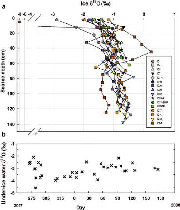
Fig. 5. (a) Water stable isotope (δ18O) versus depth in sea ice for a subset of the sampling stations. (b) Evolution of the under-ice water δ18O (sampling depths 2–5 m) during the sampling season. Adapted from Reference ChiericiChierici and others (2011).
4. Discussion
4.1. Halo-thermodynamic evolution of sea ice during the IPY-CFL study
4.1.1. Sea-ice temperature and bulk salinity
The temporal evolution of the mean sea-ice temperature (T) and bulk salinity (S i) is shown in Figure 6b and c. Trends were observed in both properties. The temporal changes observed in ice temperature and the ice temperature profiles described in Section 3.2. are typical of an annual temperature cycle of first-year ice in the Arctic, as described for example by Reference Perovich and ElderPerovich and Elder (2001). From station D1 (28 November 2007) until station D44 (6 May 2008), the profiles were similar to those previously observed in growing ice (e.g. Reference MaykutMaykut, 1982; Reference Cottier, Eicken and WadhamsCottier and others, 1999). The vertical ice temperature gradient (∂T/∂z) slackened as air temperature rose at the beginning of April (station D37). Ocean freezing temperature also appears in Figure 6b. The ice temperature profiles became near-isothermal as air temperature approached the ocean freezing temperature, which occurred around the first week of May. Further warming brought a negative vertical ice temperature gradient in surface ice of some stations (F2, F2-1 and F5), as previously observed in summer first-year ice (Reference Haas, Thomas and BareissHaas and others, 2001; Reference TisonTison and others, 2008). The evolution of the mean sea-ice temperature closely followed the evolution of the air temperature recorded during the study (Fig. 6a and b). We found a strong linear relationship (R 2 = 0.87) between the two variables as shown in Figure 7, which suggested that our ice temperature profiles were driven mainly by atmospheric forcing. Ice temperature profiles are generally driven by the surface heat balance, the oceanic heat flux and the properties of the snow cover. The oceanic heat flux is typically small in most regions of the Arctic (Reference Steele, Flato, Lewis, Jones, Lemke, Prowse and WadhamsSteele and Flato, 2000). The snow cover, which has a lower effective thermal conductivity than that of sea ice (Reference Sturm, Holmgren, König and MorrisSturm and others, 1997), can strongly influence sea-ice temperature profiles. We indicate the snow thickness of each station next to its icon in Figure 7. We observed that deviations from the linear relationship with air temperature were not correlated with the snow thickness (R 2 = 0.01). Hence it is unlikely that the snow cover strongly influenced our ice temperature profiles. This is understandable since the snow cover was typically thin and consisted most of the time of wind slab layers, which are known to have higher effective thermal conductivity relative to other snow types (Reference Sturm, Holmgren, König and MorrisSturm and others, 1997).
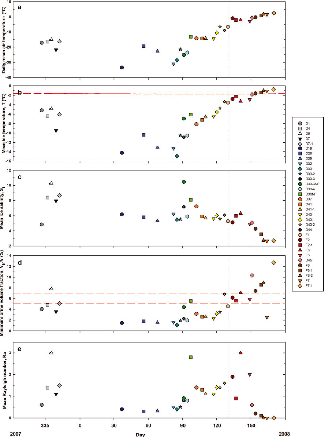
Fig. 6. The evolution throughout the sampling season of: (a) daily mean air temperature, (b) mean sea-ice temperature, (c) mean sea-ice bulk salinity, (d) minimum brine volume fraction and (e) mean Rayleigh number. The vertical dashed line indicates the start of fast-ice sampling. In (b) the horizontal dashed line is the ocean freezing temperature (T f) calculated using T f = −AS w where A = 0.054°C psu−1 (Reference AssurAssur, 1958). In (d) the horizontal dashed lines are permeability thresholds (5% and 7%) (Reference Golden, Eicken, Heaton, Miner, Pringle and ZhuGolden and others, 2007).
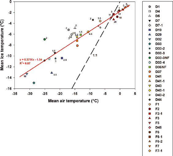
Fig. 7. The linear relationship (R 2 = 0.87) between the daily mean air temperature and the mean ice temperature recorded at the IPY-CFL stations. The snow depth (cm) measured at each station is indicated next to the icon of each station.
The evolution of the mean sea-ice bulk salinity (Fig. 6c) showed a decrease from 8–10 during the first sampling period (28 November 2007 to 13 December 2007, with the exception of station D1) to 6 on 6 February 2008 (station D19). This is easily explained. As the ice grew thicker with the progression into winter, drainage of salts at the ice–ocean interface became more efficient, decreasing the mean bulk ice salinity of the ice. From 6 February 2008 until 20 May 2008 (station F3), the mean bulk ice salinity did not vary much, fluctuating at about 6, corresponding to the quasi-steady-state salinity described by Reference Nakawo and SinhaNakawo and Sinha (1981). The mean bulk ice salinity subsequently decreased almost linearly from 20 May 2008 until 9 June 2008 (station F6-2), stabilizing at ~2.6 until the end of the sampling season (18 June 2008, station F7-1). We suggest that this desalination trend was caused by an episode of full-depth gravity drainage. In order to discuss this, we introduce in the following subsection two additional physical parameters: brine volume fraction and Rayleigh number.
4.1.2. Brine volume fraction and Rayleigh number
The brine volume fraction (V b/V) is defined as the fraction of brine relative to the bulk sea-ice volume. Gravity drainage depends actively on the connectivity of brine inclusions, which is usually simplified to be proportional to the brine volume fraction (Reference Petrich, Eicken, Thomas and DieckmannPetrich and Eicken, 2010). In brief, above a brine volume fraction of 5–7% (i.e. percolation threshold), discrete brine inclusions start to connect and the ice is considered to be permeable to fluid transport, enabling gravity drainage (Reference Weeks, Ackley and UntersteinerWeeks and Ackley, 1986; Reference Cox and WeeksCox and Weeks, 1988; Reference Golden, Ackley and LytleGolden and others, 1998). Brine volume fraction was computed from sea-ice temperature and bulk salinity using the equations of Reference Cox and WeeksCox and Weeks (1983) for ice temperature <−2°C and of Reference Leppäranta and ManninenLeppäranta and Manninen (1988) for ice temperature ≥−2°C and assuming thermodynamic equilibrium of the brine with surrounding ice. As sea-ice total gas content and sea-ice density were not measured, the air volume fraction in the equations was neglected. This approximation is acceptable for the great majority of the stations sampled since the gas volume fraction is usually negligible compared with the brine volume fraction in cold ice (Reference Petrich, Eicken, Thomas and DieckmannPetrich and Eicken, 2010). However, for warmer sea ice (ice temperatures >−5°C) the gas volume fraction can represent a significant fraction of the total volume, usually from 0 to 2% (Reference Tison, Haas, Gowing, Sleewaegen and BernardTison and others, 2002; Reference Rysgaard and GludRysgaard and Glud, 2004) although extreme values of 13% have been reported (Reference Rysgaard and GludRysgaard and Glud, 2004). Hence, the brine volume fractions computed for the warmest stations of this study are probably slight overestimates.
The porous-medium Rayleigh number (Ra) introduced by Reference Notz and WorsterNotz and Worster (2008) provides a diagnostic criterion for vertical stability within the mushy layer and is used in this study as a proxy for the intensity of brine convection (i.e. gravity drainage). At a depth z (0 at the ice base, positive upwards), it reads:
Ra was derived from sea-ice temperature and bulk salinity using the following parameters and formulas: g = 9.81 ms−2 is the acceleration due to gravity; β(S b(z) − S OC) is the density difference between brine density at a level z and that of sea water at the ice–ocean interface; S b(z) is the salinity of brine at a depth z diagnosed from temperature, assuming thermal equilibrium using Reference NotzNotz (2005) third-order fit based on the data of Reference AssurAssur (1958);S OC is the salinity of sea water; β = 0.78 kg m−3 ppt−1 is the haline expansion coefficient of sea water at 0°C (Reference FofonoffFofonoff, 1985); Π(V b/V min) is the effective sea-ice permeability (m2) computed using the formula of Reference FreitagFreitag (1999) as a function of the minimum brine volume fraction (V b = V min) between the level z and the ice–ocean interface (brine volume fraction is taken from Reference NotzNotz, 2005); and η = 2.55 × 10⁻³ kg ms−1 and κ = 1.2 × 10⁻⁷ m s−2 are, following Reference Notz and WorsterNotz and Worster (2008), the dynamic viscosity and the thermal diffusivity of brine, respectively. Based on experimental studies, Reference Notz and WorsterNotz and Worster (2009) suggest that for convection to occur, the Rayleigh number must exceed a critical value, typically 10. Physically, this means that convection only occurs once buoyancy forces due to the vertical brine density gradient expressed in the numerator of Ra overcome dissipation as expressed by the denominator.
We decided to present the depth profiles of brine volume fraction and Rayleigh number (Figs 8 and 9) since this is, to the best of our knowledge, the first time that both parameters have been computed from ice growth until the start of melt. We added dashed lines representing permeability thresholds of 5% and 7% on each of the brine volume fraction plots (Fig. 8). The percolation theory was essentially developed for ideal well-aligned columnar ice for which 5% is assumed to be a reasonable permeability threshold (Reference Golden, Ackley and LytleGolden and others, 1998). Permeability has a strong dependence on the ice microstructure, which is currently not perfectly known. For more complicated ice microstructures the threshold is presumably higher (e.g. Reference Golden, Eicken, Heaton, Miner, Pringle and ZhuGolden and others, 2007). As revealed by our thin-section pictures analysis (Fig. 4), most of the ice at the sampled stations was well-aligned columnar ice and a 5% permeability threshold is most probably applicable. However, since we looked at the ice texture and not specifically at the ice microstructure we prefer to consider a range of permeability threshold (5–7%) rather than a single value (e.g. 5%). The first sampling period from 28 November 2007 until 13 December 2007 (stations D1 to D7-1) showed brine volume fractions very close to (D1, D4, D7) or just above (D5, D7-1) permeability threshold values, suggesting that some stations were permeable early in the sampling season. As the ice cooled, it became impermeable, with brine volume fractions dropping below 5%at most depths, with the exception of the warmest bottom ice sections (5–20 cm). This was observed from 6 February 2008 (station D19) until 11 April 2008 (station D37), with the exception of the recently refrozen lead stations (D33-3NF and D36NF). The newly formed ice was warmer and more saline. When vertical ice temperature gradients started to slacken on warming, brine volume fractions increased at all depths, exceeding, or being within the range of, permeability threshold values in the bottom half of the ice. This was observed from 16 April 2008 (station D41) until 2 May 2008 (station D43-2). Further warming raised brine volume fractions slightly above 7% at nearly all depths at station D44 (6 May 2008) and well above 7% at all depths at the last drift-ice station sampled (D45 on 30 May 2008). Brine volume fractions at the fast-ice stations were always above 5%, with the exception of a surface ice layer of station F7 with near-zero salinity. From 9 May 2008 (station F1) until 28 May 2008 (station F5), the brine volume fractions were slightly larger than, or within the range of, permeability threshold values. Brine volume fraction was well above 7%after 2 June 2008 (station F6) and until the end of the sampling season.
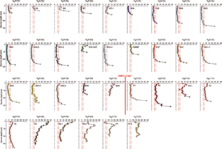
Fig. 8. Vertical profiles of brine volume fraction (V b /V) at the sampling stations. The vertical dashed lines are permeability thresholds (5% and 7%) (Reference Golden, Eicken, Heaton, Miner, Pringle and ZhuGolden and others, 2007).
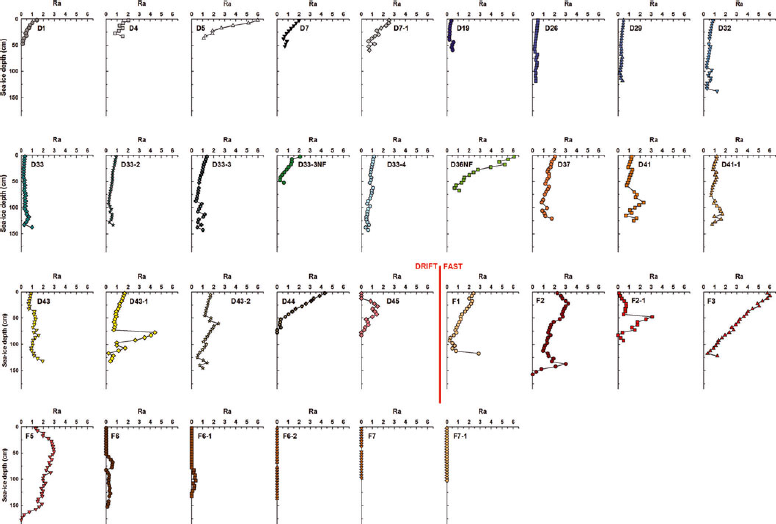
Fig. 9. Vertical profiles of the Rayleigh number (Ra) at the sampling stations.
Some discussion on the applicability of field-determined Rayleigh number profiles and critical convection thresholds (Reference Notz and WorsterNotz and Worster, 2009) is required. This became apparent once we realized that our maximum calculated Rayleigh number for this study is 6.1, well below the accepted threshold of 10. Ice coring provides a snapshot of sea-ice properties at daily or weekly intervals, while halo-thermodynamic processes can modify the sea-ice physical properties within a 24 hour period (Reference Golden, Ackley and LytleGolden and others, 1998; Reference Vancoppenolle, Goosse, de Montety, Fichefet, Tremblay and TisonVancoppenolle and others, 2010). Reference Vancoppenolle, Goosse, de Montety, Fichefet, Tremblay and TisonVancoppenolle and others (2010), using their one-dimensional sea-ice model, observed that convective instabilities can take several weeks to build, while a critical Rayleigh number can vanish within 2 days. Hence, deriving Rayleigh number from sea-ice temperature and bulk salinity using ice cores collected at daily or weekly intervals provides only a glimpse of the actual temporal variations in Rayleigh number. A second sampling issue relates to the fact that brine is lost through drainage during core extraction, which leads to underestimation of bulk ice salinity (Reference Eicken, Lange and DieckmannEicken and others, 1991; Reference Notz, Wettlaufer and WorsterNotz and others, 2005). Based upon comparisons with nondestructive measurements, Reference Notz, Wettlaufer and WorsterNotz and others (2005) found the underestimation in bottom ice salinity to range typically from 1 to 5 (>20 in some instances). Underestimations in bulk ice salinity of 1 (5) due to ice coring in the lowermost layers lead to differences in Rayleigh number that are >2 (10). Brine drainage during core extraction is particularly strong in the lower (warm) parts of the cores (Reference Notz, Wettlaufer and WorsterNotz and others, 2005) and in high-salinity core sections (Reference Eicken, Lange and DieckmannEicken and others, 1991) where brine volume fraction, permeability and hence Rayleigh number are potentially the highest. However, the error in salinity should be of a few tenths at the most when care is taken during sampling (processing cores quickly) and when the ice is colder (e.g. winter). Finally, the Rayleigh number computation relies on several parameters that are not well constrained (e.g. permeability). For all these reasons, the critical convection threshold value of 10 is probably too high when analyzing Rayleigh number profiles obtained from ice-core temperature and bulk salinity data. This is confirmed by the low Rayleigh numbers (between 0.1 and 1.9, mean = 0.8, SD ±0.5) observed in this study in the lowermost layers of growing sea ice where convection is normally expected to occur (e.g. Reference WorsterWorster, 1992). Similar low bottom-ice Rayleigh numbers were reported in field studies in McMurdo Sound, Antarctica, by Reference Gough, Mahoney, Langhorne, Williams and HaskellGough and others (2012).
We decided to plot the temporal evolution of the minimum brine volume fraction (V b /V) and mean Rayleigh number (Ra) in Figure 6d and e, respectively, and to compare these values with the temporal evolution of the mean bulk ice salinity (Fig. 6c). Since an impermeable ice layer is enough to prevent full-depth gravity drainage (and hence important desalination), we chose to plot the minimum brine volume fraction instead of the mean brine volume fraction. Also shown in Figure 6d are dashed lines representing permeability thresholds of 5% and 7%. It makes sense to plot both the maximum and mean Rayleigh number; however, since they gave almost exactly the same trends, we chose to plot only the mean. Temporal trends were observed in both parameters, and these trends seem to correspond to the mean bulk ice salinity variations. From station D1 (28 November 2007) until station D43-2 (2 May 2008), the minimum brine volume fraction remained under the permeability threshold and the potential for convection limited to the lowermost layers of the ice. The only trend in the temporal evolution of the mean bulk ice salinity, i.e. the decrease from 13 December 2007 (station D7-1) to 6 February 2008 (station D19), was the result of the increase of the efficiency of drainage at the ice–ocean interface as ice grew thicker (see Section 4.1.1). As the minimum brine volume fraction increased above 5%, as observed on 6 May 2008 (station D44), the mean Rayleigh number increased significantly, peaking at 3 by 20 May 2008 (station F3). We believe this triggered full-depth gravity drainage, which explains the strong and almost linear decrease in mean bulk ice salinity that we observed from 20 May 2008 (station F3) until 9 June 2008 (station F6-2). Thereafter, desalination stabilized the brine density profiles, decreasing the potential for gravity drainage, as suggested by the decrease in the mean Rayleigh number despite increasing minimum brine volume fraction. Sea ice eventually continued to freshen (bulk salinities approaching 0) through the infiltration of meltwater at the ice surface, as inferred by the δ18O profile of station F6-1 (Fig. 5), reducing surface salinities to close to 0. The δ18O profile of station F6-1 was particularly interesting as it showed the replacement of more negative brine by more positive pure ice melt between 20 and 60 cm depth, a process already described in summer sea ice (Reference TisonTison and others, 2008).
A few stations did not conform to the trends discussed above. Recently refrozen lead stations (D33-3NF and D36NF) had higher mean ice temperatures and bulk salinity relative to the other drift-ice stations sampled around the same time (April 2008). Sea-ice formation in leads at any time of the year is equivalent to restarting an ice growth cycle. Hence, it was not surprising to see that the physical properties of the recently refrozen lead stations were similar to those of the stations sampled in November and December 2007 (D1 to D7-1). Warm ice at stations D5 and D36NF allowed the ice to become permeable early in the season and prone to full-depth gravity drainage (mean Rayleigh number close to 3). Very low mean bulk ice salinity (4.8) was observed at station D1. Coincidentally, the δ18O values of the upper half section of station D1 (Fig. 5) were significantly less negative than those of all the other stations. Hence, we suggest that station D1 grew in slightly fresher waters than all the other stations (e.g. waters still influenced by ice melt from the previous melt season or under coastal influence).
4.2. Spatial variability
As previously mentioned (Section 2), this study involved sampling over time within small regions and across great distances, hence the data are subject to both temporal and spatial variability. We showed in Section 4.1 (Fig. 6) that temporal trends in the ice physical properties could easily be identified and linked to atmospheric forcing despite spreading of the stations across the Amundsen Gulf. This suggests that, as long as the ice floes were carefully selected (as was the case during this study; Section 2.2), the influence of regional spatial variability in the Amundsen Gulf during the IPY-CFL study may be small. That the snow-cover thickness showed little variation (Table 1) helped to mitigate the effect of spatial variability.
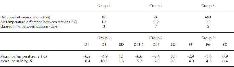
To demonstrate the fact that large-scale (regional) spatial variability was in fact small, we selected three pairs of stations and looked carefully at their ice temperature and bulk salinity profiles. The following criteria were used to select the stations: the distance between stations had to be large (a few tens of kilometers), their sampling dates and air temperatures had to be close (within a week and within 2°C) and both fast-ice and drift-ice stations had to be represented. We ended up with the three groups of data that are presented in Figure 10. Depths within the cores were normalized with respect to the total thickness (Reference Eicken, Lange and DieckmannEicken and others, 1991). Criteria used to create the groups are presented in Table 2 as well as the standard deviation in mean ice temperature and bulk salinity between stations. Standard deviations for both variables were small in all three groups and definitely smaller than the temporal variations described in Section 4.1. Also, the individual ice temperature and bulk salinity profiles are similar between floes (Fig. 10). Regarding bulk ice salinity, the standard deviation was smaller in group 2 (±0.1) than in groups 3 (±0.4) and 1 (±1.3). This was somewhat expected. Surface sea-water properties (as shown by the δ18O values of under-ice water in Fig. 5) were likely more variable in the early growth season (group 1). Growth of thick columnar ice and associated drainage limited to the ice–ocean interface (group 2) generates less variability than thin frazil-ice growth observed in the first steps of sea-ice formation (e.g. Reference Wettlaufer, Worster and HuppertWettlaufer and others, 1997). It also generates less variability than the strong desalination and surface melting mechanisms occurring later in the season (group 3).

Fig. 10. Vertical profiles of sea-ice temperature (T) and bulk salinity (S i) for each of the groups defined in Section 4.2. The curves are drawn through the midpoints of individual sections. Depth scales are normalized to unity.
Table 2. Spatial variability parameters
4.3. Sea-ice formation and deformation processes during the IPY-CFL study
4.3.1. Snow ice and superimposed ice
Most of the stations showed a textural sequence of granular texture overlying columnar texture typical of Arctic first-year ice (Reference Gow, Tucker and SmithGow and Tucker, 1990). This sequence usually corresponds to the processes of frazil and congelation ice formation (Reference Weeks and AckleyWeeks and Ackley, 1982). Granular texture is, however, also associated with the formation of snow ice and superimposed ice. Snow ice forms via the freezing of snow wetted either through flooding or brine wicking and has a fine-grained orbicular granular texture (Reference Massom, Lytle, Worby and AllisonMassom and others, 1998). Snow ice can be discriminated from frazil ice through its lower δ18O value (Reference Lange, Schlosser, Ackley, Wadhams and DieckmannLange and others, 1990). Very limited (if any) snow ice formed at the IPY-CFL stations, as generally observed in the Arctic where a thin snow cover prevails for much of the year (Reference Petrich, Eicken, Thomas and DieckmannPetrich and Eicken, 2010). Conditions favourable to flooding did not develop during the IPY-CFL study since at the maximum the snow cover represented 15% of the ice thickness and the freeboard was always positive (Table 1). The δ18O data indicate that only one value (−7.95‰ at station F6-1) was compatible with the formation of snow ice. However, this value was recorded during surface melting and therefore more likely resulted from snow meltwater infiltration. A brine skim could have been present at some stations where frost flowers were observed (D4, D5, D33-3NF and D36NF) since brine skims are known to favour the formation of frost flowers (Reference Perovich and Richter-MengePerovich and Richter-Menge, 1994). If so, it only represented a very thin layer most likely scraped off the ice surface prior to coring.
Superimposed ice forms when snow meltwater percolates and refreezes at depth in the snow cover or at the snow–ice interface (Reference Jeffries, Shaw, Morris, Veazey and KrouseJeffries and others, 1994; Reference Haas, Thomas and BareissHaas and others, 2001). As mentioned earlier (Section 3.3), superimposed ice was removed from the ice surface prior to coring, and its characteristic texture could not be detected in the ice texture analysis. From the snow observations (Table 1), we know that superimposed ice formed over a small time window, from station F2-1 (16 May 2008) until station F6 (2 June 2008). This small time window fell between the onset of melting (air temperature close to 0°C at about 9 May 2008; Fig. 1) and the onset of melt pond formation (station F6, 2 June 2008). However, while being observed over a small time window, superimposed ice layers were occasionally quite thick (1–10 cm), representing 18–100% (mean = 70%, SD ±35%) of the total snow-cover thickness and 0.5–10.0% (mean = 4%, SD ±4%) of the total ice thickness of the aforementioned stations. These percentages compare well with the percentages measured by Reference Haas, Thomas and BareissHaas and others (2001) in summer first-year ice in the Weddell Sea, Antarctica.
4.3.2. Frazil accumulation vs thermodynamic congelation growth
Based on the preceding discussion, it is reasonable to assume that the great majority of the granular texture in our thin-section pictures was frazil ice. The relative thickness of the granular and columnar texture provides insight into which sea-ice formation process (frazil accumulation or thermodynamic congelation growth) dominated at the IPYCFL stations. We observed congelation growth to have a mean contribution of 95% to the total ice thickness (vs 3% for frazil accumulation) at the three fast-ice stations (F1, F2-1 and F7-1). All but two drift-ice stations (D1 and D29) showed similar mean percentages (90% vs 7%, excluding the two aforementioned stations). These large contributions of congelation growth compare well with observations from drift ice in the southern Beaufort Sea (Reference MeeseMeese, 1989), from fast ice in the Chukchi and Beaufort Seas (Reference Weeks and GowWeeks and Gow, 1978) and from drift ice in the Fram Strait (Reference Tucker, Gow and WeeksTucker and others, 1987). It is worth noting that in Antarctic platelet ice as much as 75% of the growth of the platelet ice texture can be through congelation (Reference Gough, Mahoney, Langhorne, Williams and HaskellGough and others, 2012). Since we could not determine precisely how our platelet and draped platelet texture formed (Section 4.3.4), we did not add these textures to the congelation growth contribution. Hence, our mean contributions of congelation growth are potentially slightly underestimated.
The amount of frazil ice accumulated before congelation ice starts to grow is a function of the turbulence of surface water. From the mean contributions of congelation and frazil ice, we can deduce that at least three different growth situations occurred during the IPY-CFL study. The great majority of the ice sampled grew in calm surface waters, with congelation ice largely dominating the ice texture. This corresponds well to the low oceanic turbulence and high ice concentration (9–10 tenths) observed in the sheltered waters of the Canadian Antarctic Archipelago and Amundsen Gulf in winter (Reference BarberBarber and others, 2010). Some ice grew under extremely calm waters within leads, as illustrated by the 100% congelation ice contribution at station D33-3NF. Finally, some ice grew in more turbulent waters early in the autumn when ice concentrations in the Amundsen Gulf were lower (<8 tenths) (Reference BarberBarber and others, 2010), as illustrated by the 45% frazil-ice contribution at station D1.
4.3.3. Sandwiched granular ice layers
Thin layers (1–2 cm) of granular ice sandwiched between columnar ice were observed in the near-surface and interior ice of drift-ice stations D1, D7, D7-1, D29, D32 and D43. These layers were frazil ice because they consisted of medium to large orbicular granular crystals and their δ18O values were not overly negative (mean = −1.25‰, SD ±0.34‰) (Fig. 5). Frazil ice at depth in the ice can form through several processes: (1) rafting and ridging, (2) adiabatic supercooling in rising water masses near ice shelves, (3) double diffusion between two water masses of different properties and (4) turbulence in leads (Reference Weeks and AckleyWeeks and Ackley, 1982; Reference MaykutMaykut, 1985; Reference Tucker, Gow and WeeksTucker and others, 1987; Reference Lange and EickenLange and Eicken, 1991). We discount adiabatic supercooling and ridges because we did not sample in the proximity of ice shelves or in areas of ridged ice.
We cannot say for sure that these sandwiched layers did not result from rafting given personal observations of the prevalence of rafting in the study area, as well as documented accounts (e.g. Reference Melling, Topham and RiedelMelling and others, 1993). However, obvious signs of crystal deformation typical of rafting (Reference Jeffries, Shaw, Morris, Veazey and KrouseJeffries and others, 1994) were not widely observed. Only station D43 showed a transition from bended or tipped columnar crystals to flattened granular crystals. Also, the physical properties (bulk salinity and δ18O signal) of the sandwiched layers did not match those of surface layers, while this usually is the case in rafted ice cores. For example, double C-shaped bulk ice salinity profiles were not observed.
Double diffusion typically takes place in the Arctic in under-ice melt ponds (Reference EickenEicken, 1994) and in the presence of mixing with river water (Reference StigebrandtStigebrandt, 1981). Both processes were unlikely the source of the sandwiched layers since these were observed before melting and no riverine influence (salinity and δ18O signal) was observed in our ice-core properties.
The most plausible sources for the sandwiched layers were the leads and cracks regularly observed throughout the sampling season in the Amundsen Gulf (Reference BarberBarber and others, 2010). Frazil crystals formed within a lead through turbulence could have stirred below adjacent floes or, after the refreeze of the lead, risen back to the bottom of the ice cover with congelation growth resuming after that (Reference MartinMartin, 1981). Also, double diffusion could have occurred through thermohaline convection around intense brine plumes generated by the refreeze of ice cracks (Reference MartinMartin, 1974).
4.3.4. Platelet ice layers
Unusual textural features were observed during this study: (1) a thin layer of platelet ice (Fig. 4e) at the bottom of stations D29 and F2 and (2) a thick layer of draped platelet ice (Fig. 4d) in near-surface ice of station D29. Platelet ice forms through unrestrained frazil-ice nucleation and growth (Reference Jeffries, Weeks, Shaw and MorrisJeffries and others, 1993) and is usually associated with ice shelves and the ice pump mechanism (Reference Lewis and PerkinLewis and Perkin, 1983). In the Arctic, where large ice shelves are missing, platelet ice is very scarce and is usually associated with under-ice melt ponds (Reference EickenEicken, 1994; Reference Jeffries, Schwartz, Morris, Veazey, Krouse and CushingJeffries and others, 1995). Platelet ice in this study was found before the onset of melt-pond formation.
According to Reference Jeffries, Schwartz, Morris, Veazey, Krouse and CushingJeffries and others (1995), platelet ice in the Arctic can form through three additional processes: (1) anchor ice formation, (2) double diffusion between two water masses of different properties and (3) a small-scale ice pump involving leads and pressure ridges. We discount anchor ice formation since water depths recorded at the IPY-CFL stations (>100 m) exceeded depths at which anchor ice forms (Reference Reimnitz, Kempema and BarnesReimnitz and others, 1987) and since no sediments were found in our cores. Double-diffusion processes have already been discussed in Section 4.3.3 for the sandwiched layers and it is likely that the same processes were also the source of the platelet layers. Alternatively, platelet ice could have formed through a small-scale ice pump that operates as follows. Cold and salty water from the surface of a lead warms as it moves downwards. This water melts a small amount of ice when passing under a ridge, resulting in a layer of water fresher than surrounding waters. This layer, now at its freezing point at depth, rises and eventually becomes adiabatically supercooled with potential formation of platelet crystals (Reference Jeffries, Schwartz, Morris, Veazey, Krouse and CushingJeffries and others, 1995). Numerous leads and ridges were observed in the Amundsen Gulf throughout the sampling season (Reference BarberBarber and others, 2010). However, ridges were always located >500 m from our sampling sites.
Platelet ice was found in only 2 of the 16 cores selected for textural analyses. Hence platelet ice formation was probably not widespread in the Amundsen Gulf during the study, which compares well with previous Arctic first-year ice observations (Reference Jeffries, Schwartz, Morris, Veazey, Krouse and CushingJeffries and others, 1995). However, the mean contribution of platelet ice to the total ice thickness at station D29 (20%) suggested that this formation process was locally significant.
5. Conclusion
We have reported sea-ice temperature and bulk salinity measurements from 33 stations sampled in the southern Beaufort Sea–Amundsen Gulf from November 2007 until June 2008 during the IPY-CFL study. This represents a significant dataset covering a complete cycle from growth to the start of melt. We provide this dataset in a spreadsheet in the supplementary material (http://www.igsoc.org/hyperlink/12j148/). It represents a useful tool for the IPY-CFL community but also for future experiments in the southern Beaufort Sea–Amundsen Gulf and is a good basis for model validation.
We used this large dataset to investigate the halothermodynamic evolution of sea ice. The following trends were observed. There was a strong linear relationship (R 2 = 0.87) between the mean sea-ice temperature and the mean air temperature and no correlation (R 2 = 0.01) between the deviations from the linear relationship and the snow thicknesses measured at the stations. This is because the snow cover was typically thin and consisted most of the time of wind slab layers, which have the highest thermal conductivity of all snow types (Reference Sturm, Holmgren, König and MorrisSturm and others, 1997). The evolution of the mean sea-ice bulk salinity showed a strong desalination phase occurring over a very small time window (from 20 May 2008 until 9 June 2008). During this phase, the mean sea-ice bulk salinity dropped from 6.0 to 2.6. We suggested this phase corresponded to full-depth gravity drainage initiated by the restored connectivity of the brine network with warming in the spring. We investigated this by calculating a proxy of sea-ice permeability, the brine volume fraction, and a proxy of the intensity of brine convection, the Rayleigh number. We observed that the desalination phase started immediately after the minimum brine volume fraction rose above the permeability threshold (5–7%) and immediately after the mean Rayleigh number peaked at a value of ~3.
This is, to the best of our knowledge, the first time these two proxies have been calculated from field measurements over such a long period of time. Both proxies have been used successfully in controlled ice-growth experiments and simulations (e.g. Reference Wettlaufer, Worster and HuppertWettlaufer and others, 1997; Reference Vancoppenolle, Fichefet and BitzVancoppenolle and others, 2006; Reference Notz and WorsterNotz and Worster, 2009). This study demonstrates their ability to explain sea-ice bulk salinity trends in field measurements. Nevertheless, sampling issues related to ice coring force the reconsideration of the critical convection threshold value (Ra > 10) proposed by Reference Notz and WorsterNotz and Worster (2009). In the lowermost layers of growing sea ice where convection is normally expected to occur frequently, our data suggest looking for a critical Rayleigh number between 0.1 and 1.9 (mean = 0.8, SD ±0.5). Considering full-depth gravity drainage, we found that a mean Rayleigh number of 3 (and maximum Rayleigh number of 6) preceded a strong desalination phase. While uncertainties certainly remain about the real critical value, we showed that the Rayleigh number could at least be used as a qualitative indicator of convection. Since we presented the temporal evolution of physical parameters sampled from stations dispersed over the southern Beaufort Sea–Amundsen Gulf, we also briefly discussed spatial variability. We showed that as long as the ice floes were carefully selected, the influence of regional spatial variability in the Amundsen Gulf during the IPY-CFL study was small and therefore did not represent any obstacle to time-series studies.
Finally, we investigated sea-ice textural properties using thin-section picture analysis. This analysis shed light on the sea-ice formation and deformation processes in the southern Beaufort Sea–Amundsen Gulf during the IPY-CFL study. Most stations had a typical Arctic textural sequence of granular (frazil) ice overlying columnar (congelation) ice. Formation of snow ice was not observed. Superimposed ice formed over a small time window between the onset of melting (~9 May 2008) and the onset of melt-pond formation (2 June 2008) and sometimes had significant thicknesses representing 0.5–10.0% of the total ice thickness. The mean relative contribution of congelation and frazil ice (95% vs 3% and 90% vs 7% for fast ice and drift ice, respectively) indicated that sea ice grew mostly in calm conditions. We showed that unusual textural features also could have formed locally. Sandwiched granular ice layers, platelet and draped platelet ice were all observed. We suggested that these unusual textures resulted from turbulence in leads and double diffusion around intense brine plumes generated by the refreeze of ice cracks. However, this needs to be confirmed by further investigations.
Acknowledgements
We thank the crew members of CCGS Amundsen and scientists of the IPY-CFL study for their support. We especially thank Rodd Laing, Nes Sutherland, Brent Else, Benoît Philippe, C.J. Mundy, N. Fergus and Jens Ehn for assistance with fieldwork. Mapping was performed by Ms Geilfus from NGI (Belgium). Under-ice water salinities and water stable isotopes were provided by Brent Else and Bruno Lansard, respectively. Funding for the IPY-CFL study was provided by the Canadian International Polar Year (IPY) program office, the Canadian Natural Sciences and Engineering Research Council (NSERC Discovery Grant to T. Papakyriakou), ArcticNet – a Network of Centers of Excellence, the Canada Research Chairs (CRC) Program and the Canada Foundation for Innovation (CFI). This work was part of the BA2SICS International Program funded by Belgian FNRS-FRFC 2.4649.07 and FNRS-FRFC 2.4584.09.


