I. Introduction

A continuous profile of the Arctic Ocean ice canopy was made with 48 kHZ echo sounders mounted on a nuclear submarine. A preliminary analysis by one of us (Reference Swithinbank and KarlssonSwithinbank, 1972) discussed the measuring system, the observed ice characteristics, and some broad conclusions drawn from the study. We now report on a statistical analysis that throws light on the true mean thickness, the ridging history, the total mass of ice, and the stability of the ice cover. The data were obtained by H.M.S. Dreadnought on 4-5 March 1971 in lat. 85 90° N., long. 6-7° E.

2. Data reduction

The earlier paper described the method used to enter a sea-level base line on the records. The highest openings in the ice were joined by a straight line on the assumption that they represented patches of open water. In our analysis we have accepted this base line and have related all drafts to it. However, in surfacing six times through skylights and polynyas, it was noted by direct observations that the highest openings in the pack ice were covered by new ice, nilas, or young ice varying in thickness from 5 cm up to 30 cm. A mean line drawn through a plot of these ice thicknesses against latitude has been used to determine approximate corrections to the mean drafts for use in Tables I to III. In the diagrams, true ice drafts may be up to 30 cm greater than is shown.

A semi-automatic pencil follower measuring to 0.1 mm was used to digitize the profiles at a frequency representing one or more points per linear metre of the submarine’s track. Sections in which the speed of the submarine was varying were not used. Where there was an instrument malfunction or where an ice keel went off scale from the principal recorder (reading to 25 m draft) an independent recorder reading to a depth of 35 m was used. The submarine’s speed was averaged over 30 min periods from 10 min time marks shown on large scale automatic track plots. The speed of the recording paper was averaged over lengths representing 100 km of track on the basis of similar 10 min time marks. Computer analysis of the digitized records yielded measured values of ice draft at each 2 m interval along the track.

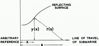
Fig. 1. Relationship between real-space coordinates (x, y) of a reflecting point on an arbitrary surface and echo profile coordinates (s,r)

The two-dimensional transformation derived by Reference HarrisonHarrison (1970, p. 1106) for the reconstruction of subglacial relief from 35 MHz airborne radio-echo sounding records was used to remove part of the distortion resulting from the nominal 20° beam of the sounder. Using Harrison’s notation (Fig. 1) we have

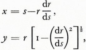
where r and s are measured and x and y are the derived horizontal and vertical distances. Given an uneven reflecting surface, the airborne sounder produced overlapping hyperbolic echoes (Fig. 2a), whereas the very dense nature of the submarine sounder trace obscured all but the first returned signals from any reflecting surface within the cone of reception. The deconvoluted ice profile as seen from the submarine (Fig. 2b) left gaps in the record representing the obscured troughs between ice keels. The best estimate of draft at these points was taken to be the minimum apparent draft on the record. This system of deconvolution was satisfactory for slopes up to 8°, just under half the nominal beam width. With greater slopes, the calculations produced a greatly distorted profile that was obviously unreal. In order to take account of the limited beam width of the 48 kHz sounder, we assumed that no energy was radiated outside the main lobe of the beam, and that energy was returned by oblique scattering from a rough surface rather than normal reflection as indicated in Figure 1.

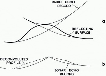
Fig. 2. (a) Hyperbolic échues on airborne radio-echo sounding record. (b) Gaps in submarine sonar record after deconvolution

By trial and error it was found that the smoothest overall profile was produced by deconvoluting bottom slopes 8°, and for greater slopes data points were shifted through 8° in a direction towards the centre of each ice keel. In other words, we assume that the first scattered return from a steeply sloping surface was received when it first intersected our beam, which had an effective half width of 8° rather than its nominal value of 10°. Figure 3 compares a section of the corrected profile with the apparent profile given by the echo trace. The net effect of our treatment has been to make the figures for overall mean ice draft about 8% smaller than those given by the uncorrected profile. If it were possible to develop a satisfactory method of deconvolution in three dimensions, we would expect a further reduction in the overall mean ice draft. If the ridges were of random orientation, we would expect the further reduction to be of similar magnitude. Such corrections do not apply to our discussions of level ice, since no deconvolution was necessary.

Fig. 3. Tracing of computer product showing original echo profile (full drawn) and corrected profile (dotted)

3. Definitions

For the purposes of this paper we have assigned special meanings to the following terms: Mean ice draft is the mean of all measured drafts including those of ice keels and open water (entered as zero draft).

Level ice. An ice draft measurement is said to describe level ice if the drafts 4 m horizontally on either side of it differ by 20 cm, implying an ice bottom slope of less than 1 in 40. Various criteria were tried (Fig. 4); this definition eliminated most of the deep draft values while being least affected by small-scale roughness.

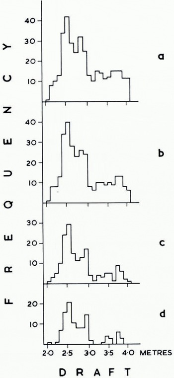
Fig. 4. Histograms of draft frequency for the same 10 km section of track. Different bottom-slope criteria were tried in an attempt to define “level ice”, (a) No points rejected, (b) Points with slope ⩾ 1 in 10 rejected, (c) Points with slope ⩾1 in 20 rejected. (d) Points with slope ⩾1 in 40 rejected

Independent keel. An ice keel is said to be independent when its maximum draft is not less than twice that of the shallowest troughs on either side of it. Ice keels with draft 5 m are excluded. This definition ensures that a broad rough keel is counted as one independent keel rather than as several (Fig. 5).

Fig. 5. Tracing of computer product showing corrected profile arid independent keels (arrowed). Crosses indicate keels excluded by the définition of an “independent keel” but included in the keel count by Swithinbank (1972)

4. Results

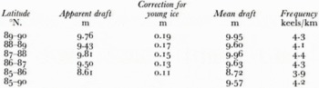
The corrected profile was analysed in 10 km sections and summarized for each degree of latitude. Mean ice draft was determined for 1 km and 1° sections (Fig. 6) to show the wide scatter of values and also for 10 km and 1° sections (Fig. 7), The 1 km means range from 0.0 m to 12.1 m, the 10 km means from 2.7 m to 6.6 m. Figure 8 shows the proportions of the track covered by ice < 30 cm draft, level ice, and ridged ice, ridged ice being interpreted as everything other than level ice having a draft >30 cm. The largest openings occurred in lat. 87° N., where as much as 21.5% of one 10 km secti4on was evidently taken by new ice, nilas, or young ice. There were substantially more openings south of lat. 87° N. than north of this latitude. One of the most revealing products analyses the draft distribution of level ice in different latitudes (Fig. 9). We do not consider that any significance should be attached to steps representing changes in frequency of <0.2%, since these could be caused by a single ice floe, but there is no doubt that the general shape of the histograms is significant. We interpret the single peak centred around a draft of 2.5 m north of lat. 88° N. as showing the preponderance of old ice in these latitudes. The lat. 87°-88° N. region evidently represents a transition zone, since within it are found the widest variations between 10 km sections (Fig. 8) with respect to ridged ice (from 51% to 87%) and also with respect to level ice (from 13% to 49%). Moreover around lat. 87° N. the first large areas of thin ice (up to 22%) are found. South of lat. 87° N. we note the progressive development of three peaks in Figure 9 which probably describe old ice (centred around 2.5 m), first-year ice (centred around 1.5 m), and ice formed during the last few weeks (<0.4m draft). Figure 10v shows the frequency distribution of ice draft measurements near the North Pole. The reason for the significant number of level ice drafts at depths approaching 10 m lies with our definition of level ice. Provided that bottom slope criteria were satisfied, the programme described any flat peak of even a deep ice keel as level ice. The break in slope at around 3 m in the level-ice curve (Fig. ioc) evidently indicates the upper limit of undeformed level ice. Table I gives the mean draft of the level ice described in Figure 9 together with a correction for the estimated mean draft of young ice.

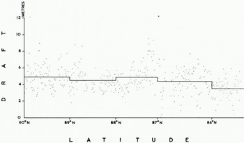
Fig. 6. Mean ice draft for 1 km sections and for each degree of latitude.

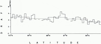
Fig. 7. Mean ice draft for 10 km sections and for each degree of latitude. Gaps indicate sections with insufficient data.

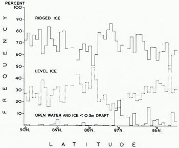
Fig. 8. Percentage of ridged ice, level ice, and thin ice in each 10 km section.

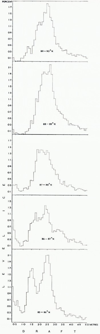
Fig. 9. Histograms of level-ice draft for each degree of latitude.

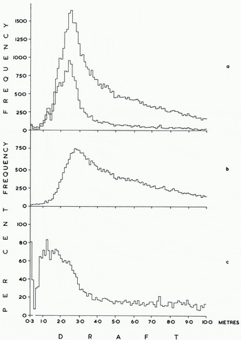
Fig. 10. Histograms of ice draft in lat. 89-90° N. (a) All ice (upper curve) and level ice (lower curve), (b) Ridged ice. (c) Level ice as a percentage of all ice.

Table 1. Mean draft of level ice between 0.3 m And 5.0 m

While the figures north of lat. 87° N. probably refer to old level ice only, south of 87° N. the figures probably describe a mean covering old, first-year, and younger ice. Figure 11 shows the very wide variations from place to place in the number and mean draft of independent ice keels. Reference Hibler, Hibler, Weeks and MockHibler and others (1972, p. 5968), who analysed comparable data from a winter voyage of U.S.S. Sargo, suggest that the statistical properties of ice keels along a given linear track can be characterized by the mean draft and mean frequency of ice keels. In the central Arctic basin over a track length of about 1 000 km they found a mean keel draft of 9.6±0.6 m and mean frequency of 4.3±1.0 keels/km. Remarkably, our data (Table II) yield almost identical results: mean keel draft 9.6 ± 1.0 m and mean frequency 4.2 ± 0.6 keels/km.

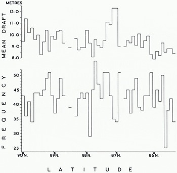
Fig. 11. Mean draft and frequency of independent keels for each 10 km section.

Table 2. Mean draft and frequency of independent ice keels.

However it is evident from Figure 11 that there are large differences between the values for neighbouring 10 km sections. We conclude that to describe average conditions satisfactorily one must average over track sections greater than 10 km in length. The same authors found a statistically significant linear correlation between the mean frequency of ice keels and their mean draft. Consequently they proposed using the mean frequency to predict the mean draft, or alternatively using the mean draft to predict the mean frequency. Our data do not support such a correlation. Indeed we find the deepest values of mean draft in an area with a low frequency of ice keels as we define them (lat. 87° N. in Fig. 11). This can be seen in Figure 12 where both Dreadnought and Sargo data are shown. The former refer to 10 km track sections whereas the Sargo data refer to 30 km sections. This leads to a greater spread of Dreadnought data, but does not explain why we find no correlation between mean draft and mean frequency.

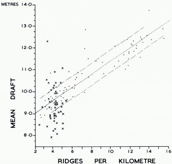
Fig. 12. Mean ice-keel draft correlated with number of i ce keels per kilometre. Dreadnought data (crosses) refer to independent keels > 5 m draft averaged over to km sections. Sargo data refer to ice keels > 6 m draft averaged wer 22-33 km sections. Linear regression line (full drawn) and standard error (dashed lines) for Sargo data. Modified from Hibler and others (1972).

The cause of this difference probably comes from our definition of an independent keel. This definition considerably reduces the number of keels in comparison with earlier counts (Fig, 5) which are probably derived in a similar manner to counts on the Sargo data. Possibly the Sargo data give an ice keel count that is approximately proportional to the total amount of deformed ice, and it would be reasonable to expect the mean draft of ice keels to be proportional to the volume of deformed ice. Studies of the upper surface by Reference Hibler, Hibler, Mock and TuckerHibler and others (1974) show a correlation between ridge frequency (definition?) and volume of deformed ice estimated from laser data. While this appears to explain the difference between the two sets of results, it must be remembered that the Sargo data cover both off-shore provinces as well as the central Arctic basin, whereas ours cover the central Arctic basin only; and for this area Hibler and others (1972) report a weaker correlation in any case.

There is no single definition of a ridge or an ice keel that will be satisfactory for all purposes. For someone driving a ship through polar pack ice, we believe our definition is the more useful; but as an indication of the mean draft of ice keels and of the amount of deformed ice it is less useful. Furthermore, the inability of the sonar beam completely to resolve high points between ice keels means that one cannot apply our definition objectively in all cases. However, this limitation applies also to other definitions such as that used by Swithinbank, where poor resolution might have an even greater effect.

Table 3. Mean draft august 1958 compared with mean draft march 1971.

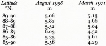
Table III compares the mean ice drafts from the trans-polar voyage of U.S.S. Nautilus in August 1958 (Reference LyonLyon, 1961, p. 670) with those from H.M.S. Dreadnought in March 1971. The Nautilus track lay within 150 km of the Dreadnought track and we would not expect such a small separation to lead to significant differences in the mean ice thickness. Furthermore we are not certain whether the Nautilus figures show mean values of ice draft excluding areas of open water, or whether they give the mean ice draft as we define it to include the whole track. When we consider all factors, we do not believe that our observations suggest that there has been a secular change in the mean thickness of the Arctic Ocean pack ice in the North Pole-Spitsbergen region during the 13 year interval between the two voyages. One likely explanation is that the Nautilus voyage was made at the height of the summer melt season, at which time a large proportion of the previous winter’s (first-year) ice would have been dissipated and there would be very little young ice. Since most of the ice would be old ice, average draft must be greater simply because there would be no younger ice to reduce the overall mean. Although in winter old floes must be thicker than they are in summer, the overall winter mean may be reduced to below the summer mean by the large stretches of young ice and first-year ice that are found everywhere during the winter.

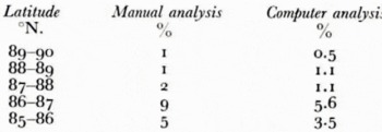
These comparisons highlight the extreme difficulty of comparing different sets of apparently similar sea-ice data. Moreover different investigators have used different definitions and different criteria for describing pack ice. Some of the problems inherent in the need to make arbitrary definitions to facilitate a particular method of reduction are shown by comparing our results with Swithinbank’s (1972) treatment of the same data. Table IV compares the percentage of track with 30 cm ice given by Swithinbank’s manual analysis and our computer analysis. Although the proportions follow the same general trend, the difference is evidently because the computer analysis interpreted the lower culminations of sinusoidal depth-holding oscillations of the submarine as thicker ice whenever they reached or exceeded 30 cm from the sea-level base line, regardless of whether or not there was any subjective indication of the presence of ice. Since any track must encounter all stages in the progressive

Table 4. Proportion of track havino ice < 30 cm.

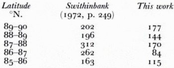
coalescence of independent ridges to become multiple composite ridges, any arbitrary definition of an independent keel must play a large part in the results of an ice-keel count. Swithinbank used the term “ice keel” to mean a keel whose draft was >10 m and was at the same time at least 5 m more than that of the shallowest troughs on either side of it. In Figure 5 we have shown that this gives rise to a larger number of ice keels and in Table V we compare the total counts of ice keel resulting from the two methods. Some authors have not defined their terms, with the result that few valid comparisons can be made with other sets of data. We conclude that faster progress could be made if methods and analyses could be standardized through the introduction of a few arbitrary but essential definitions. Standard methods of sounding and deconvolution are also needed because of the problem of resolving high points between ice keels. When such matters are agreed, the type of statistics best suited to the problem may also become clearer.

Table 5. Number of ice keels per 100 km.