


Introduction
Glacier-monitoring studies in High Mountain Asia are vital for understanding their complex degree of mass-balance fluctuations due to recent climatic conditions (e.g. Azam and others, Reference Azam2018; Maurer and others, Reference Maurer, Schaefer, Rupper and Corley2019). Studies using satellite-based digital elevation models (DEMs) have revealed continuous mass loss across the Himalaya, with the exceptions of the Karakoram and Kunlun mountain ranges, where slight mass losses or even gains have been observed (e.g. Brun and others, Reference Brun, Berthier, Wagnon, Kääb and Treichler2017; Shean and others, Reference Shean2020). Ground-based mass-balance observations across various Himalayan glaciers are therefore critical for ground truthing since the combination of individual valley climates and glacier characteristics has resulted in heterogeneous mass changes, even within the same region (e.g. Ragettli and others, Reference Ragettli, Bolch and Pellicciotti2016; Vijay and Braun, Reference Vijay and Braun2016; King and others, Reference King, Quincey, Carrivick and Rowan2017). However, in situ observational studies remain scarce due to the remoteness of these glaciers and the associated logistical difficulties (e.g. Yao and others, Reference Yao2012; Azam and others, Reference Azam2016; Sherpa and others, Reference Sherpa2017; Sunako and others, Reference Sunako, Fujita, Sakai and Kayastha2019; Angchuk and others, Reference Angchuk2021; Stumm and others, Reference Stumm, Joshi, Gurung and Silwal2021). Previous studies have employed global positioning system (GPS) and/or rangefinders during repeated surveys to derive point-based DEMs and capture surface elevation changes, and therefore estimate geodetic glacier mass balances (e.g. Fujita and Nuimura, Reference Fujita and Nuimura2011; Tshering and Fujita, Reference Tshering and Fujita2016). Precise GPS positions have also been used to validate satellite-based DEMs (e.g. Fujita and others, Reference Fujita, Suzuki, Nuimura and Sakai2008; Nuimura and others, Reference Nuimura, Fujita, Yamaguchi and Sharma2012; Berthier and others, Reference Berthier2014; Wagnon and others, Reference Wagnon2021). Furthermore, recent studies have employed uncrewed aerial vehicles (UAVs) and applied the Structure from Motion technique (SfM) to generate high-precision DEMs for glaciological monitoring, thereby allowing for detailed analyses of the morphological changes along the glacier surface (e.g. Immerzeel and others, Reference Immerzeel2014; Kraaijenbrink and others, Reference Kraaijenbrink, Shea, Pellicciotti, de Jong and Immerzeel2016; Vincent and others, Reference Vincent2016; Brun and others, Reference Brun2018; Sato and others, Reference Sato2021; Mishra and others, Reference Mishra, Miles, Chaudhuri and Mainali2021). However, these UAV-based studies have mainly been limited to debris-covered glaciers owing to the extreme atmospheric conditions in the high-elevation Himalaya. Here we report on surface elevation changes and geodetic mass balances of a small debris-free glacier in the Nepal Himalaya for a series of time intervals during the 1981–2015 period using digitised map-, GPS-, airborne- and UAV-derived DEMs.
Study site, data and methodology
Study site
The debris-free Yala Glacier (RGI60-15.03954; 28.236°N, 85.617°E) is located along Langtang Valley in the central Nepal Himalaya. Langtang Valley contains a glacierised area of approximately 120 km2, with Yala Glacier covering 1.54 km2 in 2015 (Figs. 1a and b). The elevation of the glacier ranges from approximately 5140 to 5690 m above sea level (a.s.l.), and it flows to the southwest, with a mean surface slope of 25°. Yala Glacier is one of the benchmarks in the Nepal Himalaya, as in situ glaciological and geodetic mass-balance measurements have been acquired intermittently since 1982 (Ageta and others, Reference Ageta, Iida and Watanabe1984). Several studies have revealed that the glacier has been in a state of negative mass balance in recent decades (e.g. Fujita and Nuimura, Reference Fujita and Nuimura2011; Sugiyama and others, Reference Sugiyama, Fukui, Fujita, Tone and Yamaguchi2013). Acharya and Kayastha (Reference Acharya and Kayastha2019) conducted in situ mass balance measurements for the 2011–2017 period, and Stumm and others (Reference Stumm, Joshi, Gurung and Silwal2021) updated a mass loss value of −0.80 ± 0.28 m water equivalent (w.e.) a−1, with a mean equilibrium line altitude of 5456 m a.s.l. for the same study period. Shean and others (Reference Shean2020) reported a mass loss of −0.78 ± 0.13 m w.e. a−1 for the 2000–2018 period from remote-sensing observations.

Fig. 1. (a) Regional map, showing the location of the study area (Langtang valley, red box) and Kathmandu, the capital city of Nepal. (b) Map of Yala Glacier and its boundaries in 1981, 2007, 2009, 2012 and 2015 (blue, light-blue, green, orange and red polygons, respectively). (c) Ortho image of Yala Glacier, which was generated from the 2007 aerial photogrammetry survey, with the 2009, 2012 and 2015 dGPS tracks (blue, orange and red circles, respectively) and benchmarks (red crosses) indicated. (d) Ortho image of Yala Glacier derived from the 2015 UAV photogrammetry survey, with the UAV launch site (red triangle), ground control points (GCPs, pink crosses) and camera positions (black circles) indicated. Contour lines in (b) are derived from the ALOS World 3D (30 m resolution), and the background image is a Sentinal-2 composite image that was acquired on 28 December 2015.
Differential GPS survey
In situ measurements were acquired in October 2009, May 2012 and October 2015 (Table 1). We conducted differential GPS (dGPS) surveys (GEM-1 and 2, Enabler, Inc.; and R10, Nikon-Trimble Co., Ltd.) during each measurement period. A GPS base station was installed at Kyangjin Village (28.212°N, 85.565°E; 5.5 km from Yala Glacier), with other GPS receivers roving in kinematic mode at a 1-s recording interval. The uncertainty in the dGPS systems was reported to be ~0.2 m in previous studies (e.g. Fujita and others, Reference Fujita, Suzuki, Nuimura and Sakai2008; Vincent and others, Reference Vincent2016). We established two benchmarks around the glacier (Fig. 1c). The 2009 GPS data have been evaluated by Fujita and Nuimura (Reference Fujita and Nuimura2011) and Sugiyama and others (Reference Sugiyama, Fukui, Fujita, Tone and Yamaguchi2013); here we reanalysed this dataset using our 2012 measurement. The obtained GPS records were post-processed using the RTKLIB software (http://www.rtklib.com/, last accessed on 20 May 2020) and projected onto the Universal Transverse Mercator coordinate system (zone 45N, WGS-84 reference system) as elevations above the ellipsoid (m; hereafter, elevations). The exact location of the base station was determined via the Precise Point Positioning service operated by Natural Resources Canada (https://webapp.geod.nrcan.gc.ca/geod/tools-outils/ppp.php, last accessed on 20 May 2020), with the exception of the 2009 GPS records, when a single-frequency dGPS system was employed. The 2009 GPS-DEM was co-registered against the 2012 GPS-DEM using the benchmark locations. We then generated 1 m DEMs for 2009, 2012 and 2015 by applying the inverse distance weighted interpolation function in the ArcGIS Pro software to the dGPS data and employing a search radius of $x/\sqrt 2$ (in m), where x is the resolution, based on Fujita and others (Reference Fujita2017). The grid cells with no dGPS points were systematically removed, following Tshering and Fujita (Reference Tshering and Fujita2016). The 2015 GPS-DEM was additionally resampled to 2, 8 and 10 m resolutions for comparison with the other DEMs employed in this study.
Table 1. Acquisition and resolution details of the digital elevation models employed for the elevation change calculations in this study

The 2015 GPS-DEM, which was acquired on 28 October 2015, is used as a reference DEM. The horizontal shifts of each DEM (easting and northing), and the mean, std dev. (SD) and normalised median absolute deviation (NMAD) of the elevation differences between each DEM and the 2015 GPS-DEM are provided. The SD values before co-registration are given in brackets.
a After horizontal co-registration.
b After horizontal co-registration and detrending function applied.
Aerial photogrammetry
A UAV-based photogrammetric survey, which was a component of the Gorkha earthquake-induced disaster investigation in Langtang Valley (Fujita and others, Reference Fujita2017), was conducted on 28 October 2015. A PD6-NPL hexacopter (PRODRONE Co. Ltd., Nagoya, Japan; Fig. S1), which is capable of ~15 min-duration flights, was employed for the survey. The hexacopter was equipped with a full-frame mirrorless camera (Sony α7R) that had a 36.4 megapixel sensor size (7360 by 4912 pixels) and interchangeable lens (28 mm focal length). Two flights were flown in manual mode at a mean flying altitude of ~230 m above the ground-surface, with the lines limited largely to the glacier terminus (Fig. 1d). We therefore acquired photographs of the upper part of the glacier by changing the camera angles. We placed five orange fabric sheets (1 × 1 m) at on/off-glacier areas the day before the UAV flights to obtain ground control points (GCPs). The precise GCP positions were measured via dGPS at a 1-min interval based on a similar methodology to that in previous studies (Immerzeel and others, Reference Immerzeel2014; Fujita and others, Reference Fujita2017).
We further analysed 14 oblique aerial photographs that were acquired by a private jet with two handheld cameras (Canon EOS 5D and Canon EOS-1Ds Mark2) in December 2007 to generate an ortho image and DEM. Although the exact flight height was not recorded during this flight, the mean flying altitude was estimated to be ~6700 m based on a nearby study at a similar glacier altitude that employed the same private jet (Sato and others, Reference Sato2021). We extracted 32 GCPs from specific features on the off-glacier terrain of the 2017 Pléiades-DEM and the ortho image for the 2007 dataset (Fig. S2) based on the method proposed by Sato and others (Reference Sato2021). The Pléiades-DEM was both horizontally and vertically shifted to the 2015 GPS-DEM based on the method of Nuimura and others (Reference Nuimura, Fujita, Yamaguchi and Sharma2012) and Rolstad and others (Reference Rolstad, Haug and Denby2009) (see the ‘Bias calibration’ section).
Map and satellite data
We derived the 1981 DEM from a map that was generated using ground photogrammetry images that were acquired in November 1981 (Yokoyama, Reference Yokoyama1984) to calculate the elevation changes. Fujita and Nuimura (Reference Fujita and Nuimura2011) subsequently digitised the 1981 map and interpolated it to a 10 m resolution (Fujita and Nuimura, Reference Fujita and Nuimura2011; hereafter, MAP-DEM). We re-georeferenced the digitised map and DEM to align with the key features that were detected in a Landsat image acquired in October 1988.
We further utilised the High Mountain Asia 8 m DEM (Shean, Reference Shean2017; hereafter, HMA-DEM), which was derived on 29 December 2015, to obtain the 2015 hypsometry. We also used Landsat and Advanced Spaceborne Thermal Emission and Reflection Radiometer (ASTER) images to delineate the glacier area. The satellite data used in this study are listed in Table S1.
DEM generation
SfM software (Agisoft Metashape Professional Version 1.6.0) was utilised to generate the 2007 and 2015 DEMs and ortho images following the standard SfM processing workflow (Lucieer and others, Reference Lucieer, Jong and Turner2014; Agisoft, 2020). The key details of the cameras and the SfM processing parameters are listed in Table S2. We processed 14 and 519 images in 2007 and 2015 to generate sparse point clouds with ultrahigh- and high-quality settings, respectively. We manually added GCPs to georeference the point clouds, and produced dense point clouds. We employed the ‘dense cloud confidence’ parameter, which is the number of images referenced for generating dense point clouds, to remove any outliers whose values were <2. The generated DEMs were resampled to 2 m (2007) and 1 m (2015), and the original resolution of the ortho image was exported for comparison (Table S2).
Glacier outlines
The glacier boundaries were delineated from the digitised 1981 map, 2007 aerial photogrammetry-derived ortho image, and visible or panchromatic Landsat Thematic Mapper (TM; 30 m resolution), ASTER (15 m resolution) and Landsat Operational Land Imager (OLI; 15 m resolution) bands, which were acquired in 2009, 2012 and 2015, respectively (Fig. 1b; Table S1). We excluded the DEM grids in the buffer zones along the glacier boundaries, which were defined as ±1 pixel zones in the referenced images, to clearly distinguish the on- and off-glacier areas.
Bias calibration
The DEMs used to calculate elevation changes are listed in Table 1. We first shifted all of the DEMs, including the Pléiades-DEM and HMA-DEM, horizontally (into both the easting and northing directions) to minimise the std dev. of the elevation changes between these DEMs and the 2015 GPS-DEM over the stable terrain (<30° slope) of the off-glacier area along the dGPS tracks (Nuimura and others, Reference Nuimura, Fujita, Yamaguchi and Sharma2012). We then calculated the normalised median absolute deviation (NMAD) across the off-glacier area, excluded the calculated values that were greater than ±3 NMAD from the mean values as outliers (Höhle and Höhle, Reference Höhle and Höhle2009). We further determined a first-order (linear) detrending function using a least-squares fit between each DEM and the 2015 GPS-DEM over the glacier-free terrain to remove the vertical bias, and then applied this function to both the on- and off-glacier areas (Rolstad and others, Reference Rolstad, Haug and Denby2009). The vertical accuracies (std dev.) of the DEMs ranged from ±0.11 to ±4.58 m (Table 1; Fig. S3).
Surface elevation changes and mass-balance calculations
We calculated the elevation differences for the 1981–2007, 2007–2009, 2009–2012 and 2012–2015 periods, with 2009–2012 and 2012–2015 differences based on the timing of the 2012 dGPS survey, which was conducted before the monsoon season (5–8 May 2012; Table 1). We further estimated the elevation changes for the 2007–2015 period to compare these results with those for the 2012–2015 period. We removed the outliers, which we defined as greater than ±3 NMAD from the mean elevation changes, from each 50 m band of the on-glacier area during the calculation periods. The elevation change uncertainty (σ dh) was estimated based on the standard error, which employs a spatial autocorrelation and is described as follows (McNabb and others, Reference McNabb, Nuth, Kääb and Girod2019):

where σ stable and n are the std dev. and number of pixels over the off-glacier area, respectively; L is the distance of the spatial autocorrelation (m); r is the pixel size and σ bias is the mean elevation change over the off-glacier area. L is determined by the ranges of the spherical semivariogram models that were fitted to empirical variograms of the elevation differences over the off-glacier areas using a least-squares method (Rolstad and others, Reference Rolstad, Haug and Denby2009; Wang and Kääb, Reference Wang and Kääb2015; Magnússon and others, Reference Magnússon, Belart, Pálsson, Ágústsson and Crochet2016; Ragettli and others, Reference Ragettli, Bolch and Pellicciotti2016); this value varies between 173 and 1329 m for the five analysis periods (Fig. S4).
Finally, the area-weighted geodetic mass balances (B g; m w.e.) were estimated as:

where dh z (m) is the mean annual elevation change at a given 50 m elevation band, A z and A T (km2) are the corresponding area of the mean elevation band between years t 1 and t 2 and the total area, respectively; ρ i is the ice density (assumed to be 850 kg m−3) and ρ w is the water density (1000 kg m−3; for unit conversion). We extrapolated dh z above 5500 m (~9% of the total glacier area, as the GPS-DEMs were not constrained above this elevation) via linear regression, with dh z set to zero if positive values were obtained (Sugiyama and others, Reference Sugiyama, Fukui, Fujita, Tone and Yamaguchi2013). The 1981 and 2015 hypsometries were obtained from the glacier areas and DEMs over the glacier. The HMA-DEM, which was corrected by the 2015 GPS-DEM (Fig. S3f), was used for the 2015 hypsometry calculation since the UAV-DEM covered only ~70% of the glacier area (Fig. 1d). Furthermore, we estimated the 2007, 2009 and 2012 hypsometries from the 1981 and 2015 DEMs by assuming that the hypsometry varies linearly over time (Wagnon and others, Reference Wagnon2021), because DEMs that covered the entire glacier were not available for these three years. We therefore note that the delineated glacier areas in 2007, 2009 and 2012 were not used for the B g calculations.
The uncertainties in the area-weighted geodetic mass balance (σ g) were evaluated using the uncertainties in the elevation changes ($\sigma _{dh_z}$ ), glacier area delineation ($\sigma _{A_z}$
 ) and density assumption ($\sigma _{\rho ^i}$
 ) in each elevation band, which were based on the method of Tshering and Fujita (Reference Tshering and Fujita2016):

Here we used σ dh as the elevation change uncertainty in each band ($\sigma _{dh_z}$ ). We applied the root mean square errors of the linear regression against the mean elevation changes in each elevation band as the uncertainty (~0.62 m a−1) for the areas where the elevation changes were extrapolated (>5500 m elevation). The uncertainties in the glacier area were estimated from the glacier boundaries and the DEMs in 1981 and 2015, where we assumed $\sigma _{A_z}$
 to be half a pixel for the referenced images (5 m for the 1981 map and 7.5 m for 2015 Landsat 8 OLI) multiplied by the glacier outline perimeters of each elevation band. The uncertainty in the density assumption was assumed to be 60 kg m−3.
Results and discussion
The mean annual elevation changes for the five analysed intervals during the 1981–2015 period are shown in Figure 2. A relatively higher degree of variability is observed in the 2007–2009 elevation differences of both the off- and on-glacier areas (Fig. 2 and Table S3). The elevation differences for this interval are likely more affected than those for the other analysed periods, since the 2007 DEM was generated from only 14 oblique photographs and did not capture the glacier surface features as well as the 2009 DEM did. Furthermore, the short period of DEM coverage, in combination with the lower accuracy of the 2007 DEM, resulted in a relatively high σ dh (0.24 m a−1) for the 2007–2009 elevation change compared with those from the other periods (Table S3). Glacier thinning has been observed throughout the entire study period, with enhanced thinning in recent years. The maximum annual surface lowering is found around the lower bound of the glacier (~5200 m); large variations due to melting and retreating are also observed in this region (Fig. S5). The glacier boundaries (Fig. 1b and Table S4) and hypsometries (Fig. 2) also indicate continuous shrinkage from 2.42 km2 in 1981 to 1.54 km2 in 2015, with most of this shrinkage occurring around the lower bound of the glacier. Although elevation changes, which range from −0.92 to +0.44 m a−1, have been observed along the central part of the glacier (5200–5500 m) during the 1981–2007, 2007–2009 and 2009–2012 periods, the accelerated surface lowering (~−1.83 m a−1) was observed during the 2012–2015 and 2007–2015 periods. The spatial distribution of elevation changes for the two different periods (1981–2007 and 2007–2015) also revealed enhanced surface lowering from the terminus to the central part of the glacier (Fig. 3). Figure 4 depicts both the B g calculations in this study, with −0.38 ± 0.16, −0.26 ± 0.30, −0.36 ± 0.17, −0.98 ± 0.27 and −0.74 ± 0.15 m w.e. a−1 for the 1981–2007, 2007–2009, 2009–2012, 2012–2015 and 2007–2015 periods, respectively, and the estimates from previous studies (Table 2).

Fig. 2. Altitudinal distribution of the elevation changes (50 m averages) for the 1981–2007 (light blue), 2007–2009 (green), 2009–2012 (purple), 2007–2015 (orange) and 2012–2015 (red), with the1981 (grey) and 2015 (dark grey) hypsometries also shown. Error bars denote the std dev. of the elevation differences for a given elevation band. Filled circles with error bars denote the values where the elevation change was estimated via linear regression (assumed to be zero if the value is positive) and their associated uncertainties (root mean square errors).

Fig. 3. Annual elevation changes across Yala Glacier for the (a) 1981–2007 and (b) 2007–2015 periods.

Fig. 4. Time series of the area-weighted glacier mass balances (B g) for Yala Glacier estimated from this study (black line) and previous studies (KF11: Fujita and Nuimura, Reference Fujita and Nuimura2011; SR16: Ragettli and others, Reference Ragettli, Bolch and Pellicciotti2016; FB17: Brun and others, Reference Brun, Berthier, Wagnon, Kääb and Treichler2017; JM19: Maurer and others, Reference Maurer, Schaefer, Rupper and Corley2019; DS20: Shean and others, Reference Shean2020). Open circles and the dashed line indicate the in situ mass balance (DS21: Stumm and others, Reference Stumm, Joshi, Gurung and Silwal2021). Shaded regions denote the uncertainties associated with each B g calculation. Note that the B g calculations from FB17 and JM19 were estimated using the mean elevation change profiles in FB17 and JM19 and the hypsometries from this study.
Table 2. Area-weighted glacier mass balance (B g) for Yala Glacier that were derived in this and previous studies
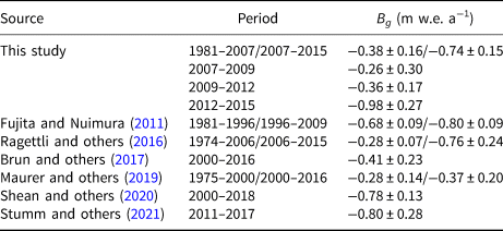
Note that the values from Maurer and others (Reference Maurer, Schaefer, Rupper and Corley2019) and Brun and others (Reference Brun, Berthier, Wagnon, Kääb and Treichler2017) were calculated using the hypsometry in this study and the 50 m binned mean elevation changes from their respective studies.
Our results indicate that enhanced surface lowering has been propagating up-glacier in recent years (Fig. 2), with this trend likely due to the imbalance in recent climatic conditions, as indicated by previous studies (e.g. Sugiyama and others, Reference Sugiyama, Fukui, Fujita, Tone and Yamaguchi2013; Ragettli and others, Reference Ragettli, Bolch and Pellicciotti2016). Previous studies have revealed the annual precipitation at Kyangjin Village (~3900 m) has varied from 647 to 924 mm since 1988 (Racoviteanu and others, Reference Racoviteanu, Armstrong and Williams2013; Shea and others, Reference Shea2015). Shea and others (Reference Shea2015) estimated the elevation of the 0°C isotherm to be ~3000 and ~6000 m during the winter and monsoon seasons, respectively, which suggests that mostly liquid precipitation falls over the glacier during the monsoon season. Such a condition would heavily reduce the opportunity for glacier accumulation and thus cause the negative mass-balance, as indicated by Stumm and others (Reference Stumm, Joshi, Gurung and Silwal2021). Furthermore, Sugiyama and others (Reference Sugiyama, Fukui, Fujita, Tone and Yamaguchi2013) attributed the surface flow velocity trend along the lower half of the glacier, where a drastic deceleration (60–90%) was observed during the 1981–2009 period, to ice thinning, which has also been confirmed for other Himalayan glaciers (Dehecq and others, Reference Dehecq2019). A decrease in the flow velocity should reduce the ice flux, and therefore induce more surface lowering due to reduced compensation via the emergence velocity (e.g. Nuimura and others, Reference Nuimura2011; Berthier and Vincent, Reference Berthier and Vincent2012; Brun and others, Reference Brun2018). These observations highlight the need to estimate and analyse the fluctuations in the long-term mass balance and emergence (submergence) velocity under recent climatic conditions, to evaluate the cause of this surface lowering in detail.
Many studies have quantified the area-weighted mass balance of Yala Glacier via in situ and/or remote-sensing approaches (Fig. 4 and Table 2). Ragettli and others (Reference Ragettli, Bolch and Pellicciotti2016) reported B g estimates of −0.28 ± 0.07 and −0.76 ± 0.24 m w.e. a−1 for the 1974–2006 and 2006–2015 periods, respectively. Fujita and Nuimura (Reference Fujita and Nuimura2011) obtained B g estimates of −0.68 and −0.80 m w.e. a−1, each with a maximum uncertainty of 0.09 m w.e. a−1, for the 1981–1996 and 1996–2009 periods, respectively, using much of the same data that were used in this study. Maurer and others (Reference Maurer, Schaefer, Rupper and Corley2019) estimated the elevation differences along glaciers throughout the Himalaya via an analysis of declassified KH-9 Hexagon satellite and ASTER images (Fig. S6). We calculated B g from the mean elevation difference profile (50 m bins) from Maurer and others (Reference Maurer, Schaefer, Rupper and Corley2019) using the hypsometries for the 1975–2000 and 2000–2016 periods, which were linearly estimated from the 1981 and 2015 hypsometries in this study, with B g estimates of −0.28 ± 0.14 and −0.37 ± 0.20 m w.e. a−1 obtained for the 1975–2000 and 2000–2016 periods, respectively. Similarly, we estimated the B g of Brun and others (Reference Brun, Berthier, Wagnon, Kääb and Treichler2017) as −0.41 ± 0.23 m w.e. a−1 for the 2000–2016 period. A comparison of the B g estimates from these previous studies indicates that our 1981–2007 B g (−0.38 ± 0.16 m w.e. a−1) is more negative than those by Ragettli and others (Reference Ragettli, Bolch and Pellicciotti2016) and Maurer and others (Reference Maurer, Schaefer, Rupper and Corley2019) although it falls largely within the uncertainty ranges of these studies; however, the time periods are not exactly the same. In contrast, the estimated B g for the 2007–2015 period (−0.74 ± 0.15 m w.e. a−1) is consistent with those by Ragettli and others (Reference Ragettli, Bolch and Pellicciotti2016), Shean and others (Reference Shean2020; −0.78 ± 0.13 m w.e. a−1 for the 2000–2018 period) and the direct measurement by Stumm and others (Reference Stumm, Joshi, Gurung and Silwal2021; −0.80 ± 0.28 m w.e. a−1 for the 2011–2017 period), whereas the estimate by Brun and others (Reference Brun, Berthier, Wagnon, Kääb and Treichler2017) is less negative than these values. The difference among our 1981–2007 B g and those of previous studies is likely due to the DEM accuracies, as the two DEMs, which are based on a 1981 map in this study and a KH-9 Hexagon image in the previous studies (Ragettli and others, Reference Ragettli, Bolch and Pellicciotti2016; Maurer and others, Reference Maurer, Schaefer, Rupper and Corley2019), may contain errors. The 1981 map was derived from ground photogrammetry using base points that were horizontally 2 km from the glacier terminus, thereby suggesting a lower accuracy over the up-glacier part (~5600 m) of the glacier due to the relatively large distance between the base points and the snow-covered area. Furthermore, satellite-based DEMs generally possess larger uncertainties that are mainly present across the poorly contrasted snowfields (accumulation area). The trend in the surface elevation changes, with the exception of that in the terminus area (~5200 m), has even varied among these recent satellite-based studies (Fig. S6). Further research, including a comparison of the KH-9 DEM in previous studies and the GPS-DEM in this study, is therefore required to better understand the DEM accuracy and B g differences before 2000. We also calculated an alternative B g using the profiles in Fujita and Nuimura (Reference Fujita and Nuimura2011) for the 1981–1996 period and the hypsometry employed in this study, which yielded a more plausible B g estimate of −0.48 ± 0.14 m w.e. a−1. This alternative calculation suggests the importance of employing a precise hypsometry for B g estimations.
Our results reveal that Yala Glacier has undergone continuous mass loss since 1981, with an unabated acceleration in mass loss in recent years, which is in agreement with previous studies along this glacier (e.g. Sugiyama and others, Reference Sugiyama, Fukui, Fujita, Tone and Yamaguchi2013; Ragettli and others, Reference Ragettli, Bolch and Pellicciotti2016; Stumm and others, Reference Stumm, Joshi, Gurung and Silwal2021) and/or the glaciers across the region (e.g. Maurer and others, Reference Maurer, Schaefer, Rupper and Corley2019). Furthermore, the estimated B g for the 2007–2015 period was more negative than both the regional mean geodetic mass balances for central Nepal (−0.46 ± 0.12 m w.e. a−1) and debris-free glaciers in the Himalaya (−0.38 ± 0.08 m w.e. a−1) during the 2000–2016 period (Maurer and others, Reference Maurer, Schaefer, Rupper and Corley2019). Small debris-free glaciers that are located at relatively lower elevations in the Himalaya have exhibited similar large mass loss trends in recent years (e.g. Tshering and Fujita, Reference Tshering and Fujita2016; Sherpa and others, Reference Sherpa2017) and would therefore suffer from an acceleration in mass loss. Stumm and others (Reference Stumm, Joshi, Gurung and Silwal2021) also mentioned that low-lying glaciers with small elevation range tend to have more negative mass balances in terms of representativeness for the regional mass balance. Although mass-balance studies have been conducted across high-elevation glaciers (e.g. Sunako and others, Reference Sunako, Fujita, Sakai and Kayastha2019; Wagnon and others, Reference Wagnon2021) and debris-covered glaciers (e.g. Dobhal and others, Reference Dobhal, Mehta and Srivastava2013; Vincent and others, Reference Vincent2016; Angchuk and others, Reference Angchuk2021) using both glaciological and geodetic methods, studies that analyse smaller glaciers, such as Yala Glacier, are necessary to better understand the responses of these small glaciers to a warming climate.
Conclusions
We analysed and re-evaluated the surface elevation changes of Yala Glacier in the Nepal Himalaya using multiple datasets, which were derived from ground and aerial photogrammetry surveys, and dGPS measurements, for the 1981–2007, 2007–2009, 2009–2012, 2012–2015 and 2007–2015 periods. Significant surface lowering was observed ~5100–5200 m, with large variations due to glacier melt and retreat. The up-glacier propagation of this surface lowering trend has been enhanced in recent years (2012–2015 and 2007–2015) compared with the earlier periods. We further estimated the area-weighted glacier mass balance, which is −0.38 ± 0.16, −0.26 ± 0.30, −0.36 ± 0.17, −0.98 ± 0.27 and −0.74 ± 0.15 m w.e. a−1 for the 1981–2007, 2007–2009, 2009–2012, 2012–2015 and 2007–2015 periods, respectively. Although relatively large mass loss was estimated for the 1981–2007 period compared with those estimated in previous studies owing to the reduced accuracy of the DEM and/or different hypsometries, the results for the other time periods, especially the 2007–2015 (−0.74 ± 0.15 m w.e. a−1) period, were mainly consistent with those estimated by the three previous studies (from −0.76 to −0.80 m w.e. a−1) using different approaches, which indicate an acceleration in glacier mass loss in recent years. Such a rapid reduction in glacier volume, as has been observed for Yala Glacier, may affect the water supply to local communities, thereby warranting the need for continuous glacier measurements using both in situ and remote-sensing data to monitor future glacier fluctuations.
Supplementary material
The supplementary material for this article can be found at https://doi.org/10.1017/jog.2022.118.
Data
The DEMs and ortho images in 1981, 2007 and 2015 that were generated in this study are available online (https://doi.org/10.5281/zenodo.7412758). The GPS data are also available from the corresponding author upon reasonable request.
Acknowledgements
We are grateful to E. Berthier for providing the Pléiades satellite data. The Pléiades stereo pair used in this study was provided by the Pléiades Glacier Observatory initiative of the French Space Agency (CNES). We wish to thank Asahi Shimbun Co., Ltd., for supporting the 2007 aerial photogrammetry survey. We express our thanks to Guide For All Seasons for their logistical support during the fieldwork and Prodrone Co., Ltd., for their dedicated UAV support. We are also indebted to all of the people who were involved in acquiring the observations during the fieldwork. Finally, we thank two anonymous reviewers and Scientific Editor J. M. Shea for their insightful comments and suggestions, which greatly improved the manuscript.
Authors’ contributions
K. F. designed this study. S. S., K. F., T. I. and S. Y. conducted the field observations with the support of R. B. K. K. F. collected and analysed the GPS data. T. I. and S. S. conducted the UAV photogrammetry survey. S.S. analysed all of the DEMs. S. S., K. F. and A. S. wrote the manuscript with the help of S. Y. All of the authors equally contributed to the discussion.


 Open access