


1. Introduction
Autonomous vehicles (AVs) are equipped with many sensors to provide information about road traffic (for more details, see Van Brummelen et al., Reference Van Brummelen, O'Brien, Gruyer and Najjaran2018). Vehicles also use high-definition (HD) maps to provide information, like vehicle location and information about the traffic ahead. The combination of HD maps and data from the car sensors enhances safety (Gaiosh, Reference Gaiosh2018; Poggenhans et al., Reference Poggenhans, Pauls, Janosovits, Orf, Naumann, Kuhnt and Mayr2018; HERE, 2019; Kourantidis, 2020). However, these benefits are impaired by the complexity of mapping. HD maps are created with expensive mapping systems (e.g. Leica Pegasus) and need subsequent manual modifications. Thus, due to the high costs, HD maps cannot be created in a conventional approach or manner (for more information, see Kim et al., Reference Kim, Cho and Chung2021).
In general, creating a map consists of two phases: (1) data collection and (2) map generation. The output of data collection is a representation of the real environment, which can be collected by different methods (e.g. laser scanning, satellite scanning, vehicle camera scanning) (Vosselman and Maas, Reference Vosselman and Maas2010; Ziegler et al., Reference Ziegler, Bender, Schreiber, Lategahn, Strauss, Stiller, Dang, Franke, Appenrodt, Keller, Kaus, Herrtwich, Rabe, Pfeiffer, Lindner, Stein, Erbs, Enzweiler, Knöppel, Hipp, Haueis, Trepte, Brenk, Tamke, Ghanaat, Braun, Joos, Fritz, Mock, Hein and Zeeb2014; Marinelli et al., Reference Marinelli, Bassani, Piras and Lingua2017; Barsi et al., Reference Barsi, Poto, Somogyi, Lovas, Tihanyi and Szalay2020). Map generation involves the processing and modification of the data from which the map itself is subsequently generated. Data can be processed and modified by humans or artificial intelligence (Jiao, Reference Jiao2018). Significant effort is required to create localisation algorithms so that the autonomous car need not be equipped with expensive sensors and HD maps will facilitate regular operation in the near future (for more information, see Shin et al., Reference Shin, Park and Park2020). Meng and Hsu (Reference Meng and Hsu2021) state that, currently, there are no criteria that would assign integrity risks to individual sensors. Seif and Hu (Reference Seif and Hu2016) state that there are two main methods to obtain data for HD maps in 3D: the first involves vehicles equipped with state-of-the-art technologies for efficient and accurate 3D road mapping (Moreno et al., Reference Moreno, Gonzalez-Jimenez, Blanco and Esteban2008); and the second uses unmanned aerial vehicle systems (i.e. piloted aircraft) equipped with lightweight sensors, such as light detection and ranging (LiDAR) or stereo cameras, to provide a new platform for photogrammetry to allow fast and autonomous data collection, a small number of errors, and dense point clouds (O'Neill-Dunne, Reference O'Neill-Dunne2015). Finding a balance between price and quality is crucial for the general implementation of HD maps. Although it is possible to create an HD map with extreme accuracy with expensive technologies and subsequent detailed human work, for practical applicability, it is necessary to assess the economic aspect. If HD maps are extremely accurate, but, as a result, no one will be able to afford them, their practical usefulness will be lost. For this reason, the trade-off between accuracy and production costs is an important factor to consider. In any case, if HD maps are considered to be another sensor, then determining the minimum necessary accuracy is a crucial step to making them customary.
All of the leading manufacturers of HD maps – CARMERA, TomTom, DeepMap, Here Technologies, Navinfo, Civil Maps, Mapmyindia, Sanborn Map Company, Navmii and Autonavi – aim to create accuracy down to units of centimetres. Various articles, research reports and studies provide specific data on the current accuracy of HD maps (for more information, see Ma et al., Reference Ma, Li, Li, Zhong and Chapman2019; Dahlström, Reference Dahlström2020; Liu et al., Reference Liu, Wang and Zhang2020; Toyota Research Institute-Advanced Development, Inc., 2020). The basis for rough AV localisation is the Global Navigation Satellite System (GNSS). This advanced technology enables localisation accuracy to the level of units of metres. However, autonomous driving requires accuracy to the level of centimetres. Increased accuracy is ensured by other technologies with which the vehicle is equipped (e.g. radars, LiDARs and stereo cameras). By combining data from these sensors with GNSS data, the location of the car can be determined to an accuracy of 10 cm (for more information, see Seif and Hu, Reference Seif and Hu2016). The basis for the exact location of the vehicle is the accuracy deviation with which the HD map is created. The German company Atlatec has set a specific accuracy of 9 cm which is able to create an HD map, see Dahlström (Reference Dahlström2020). Toyota Research Institute-Advanced Development, Inc., an automotive driving software development company, has completed the testing of concepts that demonstrate high-resolution mapping; one of the tests resulted in a relative accuracy of 25 cm at 23 locations in Tokyo and six other cities around the world (for more information, see Toyota Research Institute-Advanced Development, Inc., 2020). The same report states that HD maps can only be created to an accuracy of 40 cm using in-vehicle cameras. In contrast, the proposed method of Ma et al. (Reference Ma, Li, Li, Zhong and Chapman2019) uses an unmanned aircraft to create an HD map with images taken to a resolution of 4 cm with an accuracy of 15 cm. The study by Liu et al. (Reference Liu, Wang and Zhang2020) provides a brief overview of the most important points in the history of navigation maps and then presents extensive literature about the development of HD maps for automated driving, with a focus on HD map structure, functionality, accuracy requirements and the aspects of standardisation. It also provides an overview of the HD map accuracy parameters set by major HD map providers. The overview represents a relatively wide range – 7 to 1 m – for absolute accuracy. Note that, in the mapping community (Esri, 2019), ‘absolute accuracy is generalised to be the difference between the map and the real world, whereas relative accuracy compares the scaled distance of objects on a map to the same measured distance on the ground’.
It follows from the above that creating an HD map with an accuracy in centimetres is a very demanding discipline. Current research focuses on creating as accurate an HD map as possible, but accuracy indicators are not mentioned. The existence of research activities related to the determination of minimum accuracy requirements for HD maps is not known to the authors of this thesis. Because autonomous vehicles require positioning accuracy at both decimetres and centimetres, most current research has focused on a robust and reliable navigation solution based on several sensors (for more information, see Li and Zhang, Reference Li and Zhang2010; Meng et al., Reference Meng, Liu, Zeng, Feng and Chen2017). Table 3 of Van Brummelen et al. (Reference Van Brummelen, O'Brien, Gruyer and Najjaran2018) shows there has been a little interest in installing a stereo camera on research and commercial vehicles. In contrast, increasingly more studies focus on localisation in HD maps only using a stereo camera, see Stevart and Newman (Reference Stevart and Newman2012), Wolcott and Eustice (Reference Wolcott and Eustice2014), Neubert and Protzel (Reference Neubert and Protzel2014) and Xu et al. (Reference Xu, John, Mita, Tehrani, Ishimaru and Nishino2017). This trend expands the use of autonomy because of the low acquisition price and the sufficient accuracy (Youngji et al., Reference Youngji, Jinyong and Ayoung2018). Recently, pseudo-LiDAR has been introduced as an alternative. It is, based only on a stereo camera, but there is still a notable performance gap (You et al., Reference You, Wang, Chao, Garg, Pleiss, Hariharan, Campbell and Weinberger2019). Tesla bet on technology for automated driving based only on the camera vision.Footnote 1
Technology developed in the aerospace industry has contributed in terms of location (for more details, see Shin et al., Reference Shin, Park and Park2020). This transfer of successful and advanced applications from civil aviation was originally introduced into autonomous vehicles as a definition for the integrity risk and the level of protection to evaluate safety (for details, see Joerger and Spenko, Reference Joerger and Spenko2018; Changalvala and Hafiz, Reference Changalvala and Hafiz2019). It is, however, clear that the requirements for navigation safety are more strict for ground operations. Let us introduce two important terms: the ‘Alert Limit’ (AL) is one of the commonly used terms in aviation that has been transferred to autonomous driving. In general, an AL is a user-set parameter that provides an early warning for a deviation from normal conditions that, if exceeded, should lead to increased attention or a corrective action; the ‘Protection Level’ (PL) defines an area (one-, two- or three-dimensional) that is calculated by a user (i.e. an autonomous vehicle) within a specific coordinate system that starts in the actual navigation state (i.e. actual position, speed, orientation) and, with a very high probability, includes the navigation state indicated by the system. In other words, the PL is the area near the car where the actual dimensions of the car are oversized.
We consider the necessary condition for the priority of HD maps (i.e. the minimum accuracy to enable the operation of autonomous technologies and not adversely affect safety) to define the interval for the accuracy of HD maps, which would provide a generally valid condition for their creation. This condition for accuracy is established on the physical possibilities of the technology. In other words, the content of the work is not motivated by the study of the accuracy of different algorithms. Algorithms should meet this condition to evaluate their applicability (Jeong et al., Reference Jeong, Cho and Kim2020). First, we determine the worst possible deviation at which the creators of HD maps are closest to reality. Second, we address the addition of another inaccuracy, which is caused when locating the vehicle (i.e. using the HD map). Then, we examine the overall inaccuracy in terms of the engineering design of the communications and standards.
2. Map quality
We can evaluate the quality of maps from several points of view. The first criterion is accuracy. This metric applies to traditional maps as well as HD maps. The second aspect is the ability to locate an autonomous vehicle on an HD map, which allows comparison only for HD maps. Another criterion is security against external attacks. However, this criterion is not subject to our interest and more information is provided by other studies (Linkov et al., Reference Linkov, Zámečník, Havlíčová and Pai2019; Luo et al., Reference Luo, Cao, Liu and Benslimane2019; Moussa and Alazzawi, Reference Moussa and Alazzawi2020).
2.1 Map accuracy
At the beginning of the 20th century, paper maps began to be used for automobile navigation. The first automobile map was published by the American Automobile Association (AAA) as early as 1905 (Ristow, Reference Ristow1946; Bauer, Reference Bauer2009). There was almost no requirement for accuracy (Liu et al., Reference Liu, Wang and Zhang2020). The advent of digital maps brought requirements for accuracy. Digital maps date to the 1960s and they are associated with the first Geographic Information Systems, especially in North America. The best known systems included SYMAP, ODYSSEY, GRID, MAP and MIDAS. In the 1970s, Esri's ARC/INFO appeared on the market as one of the first vector programs. Digital maps have been common since the 1990s and their accuracy ranged from 5 m to 10 m. In 2000, deliberate degradation of the Global Positioning System (GPS) ceased, allowing civilian users to achieve up to 10 times more accurate positioning. This expanded support for digital maps included support for advanced driver assistance systems. In 2007, Toyota introduced Map on Demand, the world's first-of-its-kind technology for distributing map updates to car navigation systems. The following year, in 2008, Toyota was the first to combine the functions of a brake assist system and a navigation system that was connected to adaptive variable suspension (i.e. NAVI/AI-AVS) in its Toyota Crown model. This extension affected the required accuracy for the maps, which was 50 cm. In 2010, HD maps appeared, which, unlike the previous iterations, are processed in 3D and require an accuracy of 10–20 cm (for details, see Liu et al., Reference Liu, Wang and Zhang2020).
High demands are placed on HD maps. As a result, their creation and maintenance are demanding and expensive. Maintenance (i.e. updating) is perhaps even more complicated than the initial creation because the HD map requires quality data that are supplied quickly and cheaply.
We can achieve these conflicting requirements with the Medium map (‘MD’ map), a term introduced by Carmera (Sorrelgreen, Reference Sorrelgreen2021). Whereas the HD map is characterised by its high accuracy for traffic, the surrounding elements and spatial accuracy, the MD map provides high accuracy for elements, but with lower spatial accuracy. The MD map, thus, divides the dense and complex information of HD maps into more manageable blocks. Each of these blocks has a different degree of accuracy due to the complexity of the traffic. For example, a block that includes an intersection can be constructed and maintained with HD map accuracy, while a block that contains a motorway can be created with lower accuracy because transport through this block is easier. Thus, these logical units hold different levels of trust. The MD map records all of the elements in the block (i.e. traffic lights, pedestrian crossings, cyclists), but not their exact location in the real world (for more information, see Sorrelgreen, Reference Sorrelgreen2021).
It is possible that an MD map, which is considered theoretical, would fill the gap between the extended digital map and the HD map, as shown in Figure 1, where a digital map (i.e. SD map) focuses on the discovery of the topology of maps, such as the road network, and does not usually contain lane level information, see Ort et al. (Reference Ort, Walls, Parkison, Gilitschenski and Rus2022). They only require a relatively low-resolution image with roughly metre-level accuracy.
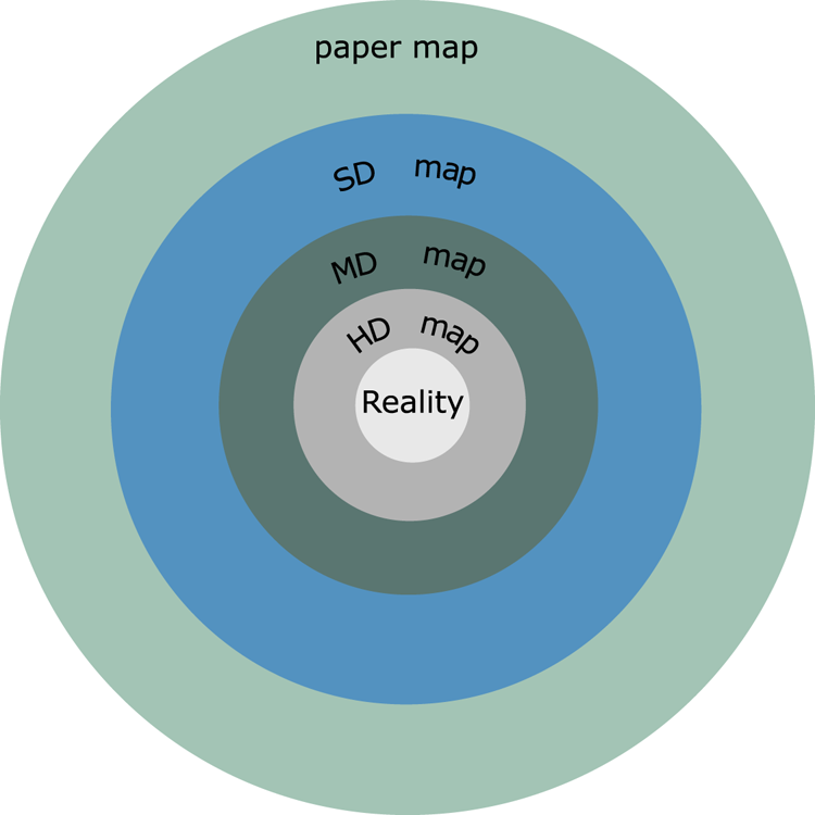
Figure 1. Types of maps arranged according to their accuracy
2.2 Factors that influence the location of the vehicle in an HD map
Today, the accurate and reliable localisation of an autonomous vehicle is perceived to be fundamental. Highly accurate localisation, in combination with an HD map, will cause a less demanding perception and an understanding of the traffic environment for autonomous vehicles (for more information, see Liu et al., Reference Liu, Li, Tang, Wu and Gaaudiot2008; Javanmardi et al., Reference Javanmardi, Javanmardi, Gu and Kamijo2018; Shin et al., Reference Shin, Park and Park2020; Endo et al., Reference Endo, Javanmardi, Gu and Kamijo2021). As mentioned above, the standard approach is to use GNSS, which is relatively affordable and reliable in open spaces. The disadvantage is in the urban environment or when the surroundings include vegetation because the accuracy decreases due to the indirect view and the reflectivity of the signals (for details, see Alam et al., Reference Alam, Kealy and Dempster2013; Iqbal et al., Reference Iqbal, Georgy, Abdelfatah, Korenberg and Noureldin2013; Yozevitch et al., Reference Yozevitch, Ben-Moshe and Dvir2014; Heng et al., Reference Heng, Walter, Enge and Gao2015; Javanmardi et al., Reference Javanmardi, Javanmardi, Gu and Kamijo2018; Arman and Tampere, Reference Arman and Tampere2021).
In the rest of this section, for the sake of completeness, we present the criteria for the evaluation of HD maps, which are described in detail by Javanmardi et al. (Reference Javanmardi, Javanmardi, Gu and Kamijo2018). Each HD map can be evaluated according to the following criteria:
• functional adequacy of the map;
• layout of objects on the map;
• local similarity;
• representative quality.
2.2.1 Functional adequacy of the map
Each HD map can be created in different ways with different algorithms. Therefore, the HD map comparison technique is based on the comparison of attributes that depend on the method of creation (e.g. in a point cloud, the attributes are the points themselves; in an occupancy-based map, the attributes are occupied cells). For better localisation accuracy, more quality attributes are required such that the quality is variable across the data file. For example, in an urban environment, there are many buildings and other structures that generate many map functions (i.e. attributes). In contrast, there are not so many objects and structures in an open field, so the map need not contain as many attributes. For this reason, it follows that the accuracy of laser-beam localisation is higher in an urban environment. Three factors are proposed to formulate the adequacy of the function: feature count, dimension ratio and occupancy ratio. These are described in detail in Section IV of the paper by Javanmardi et al. (Reference Javanmardi, Javanmardi, Gu and Kamijo2018).
2.2.2 Layout of objects on the map
In addition to the number and quality of objects, an important factor is their location in space. In fact, the concept of function distribution comes from GNSS. If a GPS-based location does not have an even distribution of satellites (i.e. the satellites are grouped), then the calculated position will be incorrect (see details in Jwo, Reference Jwo2021). Prompted by this possibility, Javanmardi et al. (Reference Javanmardi, Javanmardi, Gu and Kamijo2018) defined the factor for the formulation of the distribution of elements in the foundation of the map. The basic idea is illustrated in Figure 2, (initially introduced by Javanmardi et al., Reference Javanmardi, Javanmardi, Gu and Kamijo2018), where, in Situations 2(a) and 2(b), the vehicle is erroneously located in the longitudinal direction, while in Situation 2(c), it is possible to achieve localisation in the longitudinal direction.

Figure 2. Basic idea for the formulation of the distribution of elements in the foundation of the map. (a) Erroneously located. (b) Erroneously located. (c) Correctly located
2.2.3 Local similarity
The environment, like the abstraction shown on the map, can cause local similarity and, if the abstraction ratio is too large, the map loses detail and the local similarity increases. In other words, some points on the map have similar properties in different environments and, with increased abstraction, it is no longer possible to distinguish objects, see Figure 3.

Figure 3. Map detail
2.2.4 Representative quality
One of the most important criteria, which is directly related to the map format and the abstraction ratio, is the representative quality of the map. This factor shows the similarity of the map to the real world. On one hand, this quantity depends on the properties of the scanning technology used in the initial, scanning phase (i.e. number of beams fired by LiDAR, number of layers, scanning frequency, number of sensors). On the other hand, the quality of the map depends on the selected map format (i.e. the method of encoding to determine how the data are stored). In fact, the representative quality of the map indicates how close the map is to the original data set (i.e. the point cloud). Note that the above criteria are designed to use sensors that involve LiDAR, but not every autonomous car needs to be equipped with the same sensors (e.g. autonomous vehicle testing in Israel and South Korea use different sensors, and Telsa vehicles do not use LiDAR). These vehicles are then oriented mainly through data obtained from the camera, see Endres et al. (Reference Endres, Hess, Sturm, Cremers and Burgard2014).
3. Our solution
The analysis mentioned above shows that HD map manufacturers are able to create these map materials with different levels of accuracy. In this section, we will focus on setting the minimum required accuracy for HD map users. In other words, we will estimate the limit at which the operation of an autonomous vehicle is still safe. Below, we distinguish between the user and the creator of the HD map, where the term ‘creator’ means the whole process of creating HD maps (i.e. from data collection to the neural network algorithms to the final product).
3.1 Margin of error during creation
An accurate map is essential for orienting and determining the position of the vehicle. It is important to accept that the actual data collection and mapping includes a margin of error. The accuracy of maps is affected by several factors:
• global accuracy error ($E_{glob}$
 );
);• local accuracy error ($E_{locacc}$
);• local sampling error ($E_{locamp}$
).


Each of these factors is affected by additional aspects: the global accuracy error depends on the recording of the car location and the GPS delay (i.e. reflectivity); the local accuracy error is affected by the sensors on the AV itself, the AV speed and the ability to accurately target the object; and the local sampling error depends on the accuracy of the processing and the model creation. As mentioned above, HD map makers create maps with varying accuracy. It can be seen that the company Atlatec provides specific data for individual factors (Dahlström, Reference Dahlström2020). Specifically, the global accuracy error is less than 3 cm (i.e. $E_{glob} < 3$ cm), the local accuracy error is less than 2 cm (i.e. $E_{locacc} <2$
 cm) and the local sampling error is less than 4 cm (i.e. $E_{locamp} < 4$
 cm).
cm).
Thus, it can generally be stated that for the creation of an HD map, the parameters for $E_{glob}, E_{locacc}$ and $E_{locamp}$
 are given in centimetres. This is in line with the overall data provided by the other companies mentioned above. The total error for HD mapping is given as the sum of the maximum deviations of these factors:

Figure 4 illustrates the factors that affect the accuracy of an HD map as it is created by a recording vehicle. It is clear that the total deviation is the sum of the deviations of the factors that affect the accuracy because the position of a landmark depends on the location from which the landmark was observed by the vehicle. Other inaccuracies increase with the creation of the HD map. Note that there is a possibility for error cancellation (i.e. if the landmark is located with an error, like 5 cm to the right of the actual location) and when, conversely, the processing margin of error is from the other direction such that the two cancel each other out. Unless otherwise specified, we will continue to work with the worst possible inaccuracy.

Figure 4. Accuracy errors when creating an HD map
3.2 Margin of error for the static model
If we want to estimate the minimum necessary accuracy for an HD map such that the autonomous vehicle, according to its navigation, is able to move safely on the road network, we must work with the errors that occurred during its creation. The following estimate for the minimum required accuracy is based on HD map layers and additional data/limits. We determine the factors that will limit the accuracy of the HD map.
Below is an overview of the layers of the map, with a list of elements contained in each:
• the Geometric map layer contains roads and a geometric representation of lines in space;
• the Semantic map layer includes landmarks, lanes, curbs, intersections, traffic signs and traffic lights, the deceleration threshold, pedestrian crossings, properties of elements that affect traffic, road direction and two-way roads, speed limit, and lane departure restrictions;
• the Map Priors layer includes the order of the traffic lights at an intersection, the average waiting time for traffic lights at a given time and the probability of parking space occupancy;
• the Real-time layer includes the current traffic information and information sharing between traffic participants.
Autonomous vehicles will need to work with different levels of accuracy for the Map Priors layer and the Geometric layer, because it is clear that information about the traffic density in a given section and at a given time will not require as much accuracy as the information necessary for passing through intersections or narrow roadways (Figure 5).

Figure 5. Layers of an HD map, taken from Chellapilla (Reference Chellapilla2018)
The most restrictive conditions for accuracy are placed on the Geometric layer on which the vehicle moves. For an estimation based on the Geometric layer, it is necessary to consider the parameters of the design categories for roads, similar to that by Meng and Hsu (Reference Meng and Hsu2021) and Reid et al. (Reference Reid, Houts, Cammarata, Mills, Agarwal, Vora and Pandey2019). These parameters may be different for different countries, so we will maintain a general approach and only some situations will be demonstrated with specific examples. Figure 6 shows how the design parameters of roadways are defined.

Figure 6. Design categories of two line road, where $a$ is the width of the lane; $b$
 is the categorical width of the road; $c$
 is the width of the hard shoulder; $e$
 is the width of the shoulder; $v$
 is the edge of carriageway marking
Next, we will focus mainly on the parameter ‘$a$ ’ (i.e. the width of the lane). This width depends on the proposed speed. In the Czech Republic, widths from 2$\,{\cdot }\,$
 75–3$\,{\cdot }\,$
 50 m are established for speeds of 50–90 km/h, respectively.
This geometric view allows us to determine the deviation of the HD map, $\mu _m$ , as follows:

where $s_v$ is considered the width of the vehicle (including the PL). Equation (3.2) corresponds to the formula of Meng and Hsu (Reference Meng and Hsu2021) and Jeong et al. (Reference Jeong, Cho and Kim2020), which determines the PL for driving in a directional curve. It follows that the accuracy of the HD map may depend on the type of road. Figure 7 shows the established estimate for the minimum required accuracy and other parameters considered for lanes.


The Semantic layer of the HD map contains objects that perform the function of a landmark (i.e. points according to which the autonomous vehicle is located in the HD map, and thus also in space). It can be shown that the margin of error for the sensors and the margin of error for the computational algorithm have a significant effect on the accuracy of the localisation, while the margin of error for the location of the landmark is negligible. This is evident from the computational algorithm of triangulation for the distance from a certain object. Figure 8 shows the principle of the passive triangulation method.

Figure 8. Principle of passive triangulation
Camera A focuses on Object C at alpha and Camera B focuses on Object C at beta. Because the distance between the cameras is known, a formula for the distance of Object C can be derived according to the basic properties of a triangle:

When locating an autonomous vehicle in an HD map, active methods are also used such that the distance is determined with a combination of LiDAR and a camera. The camera focuses on the subject and LiDAR measures the distance between the subject and the car, see e.g. Wen et al. (Reference Wen, Tang, Liu, Qian and Fan2023). This active method can be considered to be more accurate than calculating the distance with two cameras. However, as mentioned above, not every autonomous car is equipped with the same sensors. Therefore, we focus on a less accurate method for localisation. By generalising Equation (3.3) for the case where the distance of the object is not perpendicular to the line between the cameras, we have a new formula for the calculation:

where $a={d\,\cdot\, \sin \alpha }/{\sin (180^\circ -\alpha -\beta )}$ and $b={d\,\cdot\, \sin \beta }/{\sin (180^\circ -\alpha -\beta )}$
 . Figure 9 shows the distance between the autonomous vehicle and the landmark. At least two landmarks are required for localisations. In the case of a higher number, the least-squares-approximation method is used to determine the position.

Figure 9. Distance from landmarks
The distance d between the cameras on the car is constant. The inaccuracy in the distance $l$ is mainly caused by the estimation of angles from the camera. This is one of the major problems for determining the position based on an image (i.e. distortion). The percentage of image distortion expresses the ratio between the real and the expected distance from the centre of the image in pixel coordinates. It is, therefore, necessary to calibrate the cameras (i.e. intrinsic matrix) to reduce this error. Table 1 shows the relationship between the degree of distortion and the margin of error for the estimated position at the camera's field of view at $90^\circ$
 . The distortion caused by the quality of the sensors (i.e. camera quality) acquires linear characteristics. At present, the quality requirements for the individual sensors with which the autonomous vehicle is equipped are not specified (for more information, see Meng and Hsu, Reference Meng and Hsu2021).
Table 1. Relationship between the degree of distortion and the error of the estimated position

We consider landmarks placed with the $E_{making}$ error (which can be neglected for insignificance) when locating the $E_{dis}$
 distortion error, and we further assume that the distortion affects the position estimate, as shown in Figure 10. The magnitude of the localisation error depends on angle alpha (i.e. the angle between Landmark 1, the detection point and Landmark 2). If the angle alpha is small, the area in which the autonomous vehicle is detected increases. If the angle alpha approaches $90^\circ$
 , the detection area $m$
 is small. This idea is from the Geometric Dilution of Precision (GDOP), where GDOP represents the geometric effect on the relationship between measurement error and positioning error. The GDOP value is calculated by an inversion matrix. The basis is the vector distance from the satellite to a located object. GDOP indicates how the distribution of satellites affects accuracy; in other words, a smaller value represents satellites that are in optimal positions and higher values indicate that the satellites are grouped. For example, a GDOP of less than $1$
 is the highest possible confidence level to be used for applications that demand the highest possible precision at all times. Inspired by GDOP ideas, we propose determining $m$
 in Equation (3.6) (i.e. the largest possible error for the location). Specific values are given in Table 2. Subsequently, we can, for the first time, determine the inaccuracy in the creation of the HD map as $\delta$
 , which satisfies the following inequality:

where


Figure 10. Angle-dependent localisation for angle alpha
Table 2. Value $m$ for distortion $1\%$
 and landmarks from camera 20 and 5 m

Note that the value of $m$ is obtained from the linearised region of Figure 10. We demonstrate our considerations above for a specific situation in a static model: a lane width $a = 350$
 cm and a vehicle with a width $s_v = 250$
 cm (which includes the PL). From Equation (3.2), we can easily determine that $\mu _m = 50$
 cm. The error caused by $1\%$
 distortion at a distance from the landmark (L2) of 20 m and a distance from the landmark (L1) of 5 m is approximately 16 and 4 cm, respectively, when the angle alpha is $70^\circ$
 . Then it follows from Equation (5) that an HD map can be created for a given section with a minimum required accuracy of $32$
 cm. Further, note that using a larger number of landmarks can provide more points to represent the vehicle. In other words, the area at the point of localisation in Figure 10 decreases more and the value of $m$
 also decreases. Note that for an infinite number of points, the area in Figure 10 was represented by the circle and $m$
 was the radius of the circle. Because we estimate the minimal required accuracy, we chose the worst possible situation for the estimation. In our case, therefore, we considered only two landmarks, and solved the error for the most important lateral direction, even though the other directions are also influenced. More specific values are provided in Table 4, where we consider $s_v=200$
 cm for future autonomous vehicles.
Compare the values of $m$ and $m'$
 from Tables 2 and 3, respectively. The distance of the landmark affects the value of $m$
 , but the trend of the size of the angle is the same for both tables. Note that some extreme positions of landmarks are not achievable in the practical world, e.g. $\alpha =20^\circ, L_1=20$
 and $L_2=20$
 m.
m.
Table 3. Value $m'$ for distortion $1\%$
 and landmarks from camera 20 and 20 m

Table 4 shows the minimum required lane-width accuracy for a vehicle width ($s_v = 200$ centimetres). It is clear that high inaccuracy cannot be considered for very narrow lanes because the HD map would not be able to make sense of the data. This depends on other design parameters, such as the number of passing cars. In the case of freight transport, the situation is further complicated in narrow sections because real traffic experience suggests the need for complex evasive manoeuvres. In these situations, even an absolutely accurate HD map would not be effective. The solution could provide car to car (C2C), or infrastructure to car (I2C). For example, Nordic countries specifically identify places to avoid on some roads and sometimes there is only one vehicle allowed in places on a two-way road. This avoidance manoeuvre is a matter for other algorithms. For standard lane widths from $300$
 cm, the minimum required accuracy of the HD map is 31$\,{\cdot }\,$
 41 cm, which is shown in Table 4. Current technologies make it possible to create an HD map that is more accurate. A subject for further research is how to work with the accuracy of HD maps and the PLs of autonomous vehicles. Meng and Hsu (Reference Meng and Hsu2021) shows a technique for determining the PL, which is maximised to the overall width of the lane. A subject of interest may also be a study where the PL will be used more to avoid collisions and the creation of HD maps will depend only on the actual width of the vehicle.
Table 4. Minimum required accuracy for HD maps for $m=0\,{\cdot }\,1859$ cm
cm

3.3 Margins of error for the dynamic model
Driving speed can significantly affect the location of a vehicle. Cameras capture 10–15 frames per second (FPS) in high resolution. At higher speeds, a car is able to travel up to 36 m in one second, so shooting takes place after approximately 2$\,{\cdot }\,$ 5 m. It is possible to reduce the resolution, but this is closely related to the quality of the HD maps. Another option is to reduce the speed or buy more expensive cameras with a higher frame rate. At higher speeds, the photo will be blurry or the shutter speed will need to be shortened, which will affect the quality in poor lighting conditions. A poor-quality photo reduces the success of landmark detection and classification. If we have more observed landmarks, then the probability for correct detection increases, while the method of least squares solves the calculation for the point that represents the vehicle. Figure 10 shows the number of shots per 100 m as a function of the speed when shooting at 15 FPS. Specific values are shown in Table 5.
Table 5. Number of frames according to vehicle speed

The number of frames on a given section decreases exponentially depending on the increasing speed, see Figure 11.

Figure 11. Number of frames per 100 m according to speed, where n$_{\mbox {F}}$ is the number of frames for 100 m
From a review of the available literature, if the source is cited, the tolerance for accuracy in the longitudinal direction is higher for HD map makers. However, the resulting localisation depends not only on the density of images captured by the camera but also on the speed of the computational algorithm. Therefore, a moving automated vehicle requires a high rate of position updating. For some systems, that means up to 200 Hz (Levinson et al., Reference Levinson, Montemerlo and Thrun2007), or 10 Hz with a speed limitation of 63 km/h (Levinson and Thrun, Reference Levinson and Thrun2010), or 20 Hz with a speed limitation of 60 km/h (Cui et al., Reference Cui, Xue, Du and Zheng2014). From these data, we are able to determine that the time of the computational algorithm that was designed to determine the position is from 5 to 100 ms. Then we are able to calculate that a car at a speed of 130 km/h and with a computational algorithm speed of 5 ms travels 18 cm during the calculation, and a car at a speed of 60 km/h with a computational algorithm speed of 0$\,{\cdot }\,$ 1 s travels 160 cm. If we add the distance that occurs between taking pictures at speeds of 130 and 60 km/h to both values, then we get that the vehicle is located at 268 and 261 cm, respectively. The error of estimating objects from the $E_{dis}$
 camera was considered above in the lateral direction. Due to the calculated data in the longitudinal localisation, this error has a minimal effect. At a high frequency (i.e. 200 Hz and a speed of 50 km/h), the vehicle travels approximately 7 cm during the calculation with a shooting at 0$\,{\cdot }\,$
 92 m. This provides sufficient accuracy in an urban environment. From the point of view of the planar sections of the location at which this delay appears on motorways, it is not a major problem. This aspect will have a negative effect on directional arcs. The problem of delayed localisation is demonstrated in Figure 12, where the vehicle is actually at Point B while the evaluation of its position is at Point A.

Figure 12. Parameters of horizontal curve
If the vehicle was strictly driven according to the HD map, it would start to turn with a delay. The stated deviation $o$ can then be expressed as

where

If we consider a deviation in the longitudinal direction of 268 cm at a speed of 130 km/h, which is allowed only on a highway, then the minimum radius of the directional curve is 1,025 m. Due to the sufficiently large $r$ , we consider it to be a line instead of a circular arc, because the error is of the order of micrometres. From Equations (3.6) and (3.7) for the given values, we get $o= 24\,{\cdot }\,799$
 mm.
mm.
Incorporating the results of the dynamic model into the requirements for the minimum necessary accuracy of HD maps from the static model leads to the modification of the original Equation (3.5) to

Thus, we have determined a new formula for calculating the minimum necessary accuracy for HD maps, while including several factors, i.e. design parameters for roads, camera properties, computing power and location of landmarks. However, for large values for road-design parameters and the low computational time of the algorithm, the parameter $o$ is negligible in Equation (3.9).
Note that although the modification of the formula was caused by the considerations of the passage of an autonomous vehicle through a directional curve, it is possible to use this modification in general (i.e. in directional curves and on straight sections) because it follows from the formula that, on the straight section, $o = 0, \gamma = 0^\circ$ and $u = v$
 . Then we get the following with Equation (6):

To some extent, we have already shown that longitudinal inaccuracy affects the lateral in terms of vehicle location. In the dynamic model, the speed-dependent localisation delay affects the lateral accuracy mainly in the directional arcs, or their design parameters.
4. Discussion
Determining the minimum required accuracy for HD maps depends on several factors for which the values are not precisely determined. Specifically, it is the width of the autonomous car and the associated PL. In the estimate, we assume the width of a fully autonomous car to be similar to that of a car driven by a human but a change in this parameter can fundamentally affect the required accuracy of HD maps. The width of the lane is also related because it can be different for full autonomy. The distortion of the camera system fundamentally affects the location of the vehicle, although there are no limits or requirements for the camera systems of autonomous vehicles. In our solution, the values that most correlated to real situations were used. Moreover, the estimate above is made on the basis of technical and physical dispositions, and it is not based on specific algorithms, so as not to favour any of the algorithmic solutions. Above all, the triangulation method was used for a stereo camera. Another way to estimate the depth with a mono camera was not used (i.e. one camera and measurements of the distance between shots), but the functionality is similar to a stereo camera, see Caselitz et al. (Reference Caselitz, Steder, Ruhnke and Burgard2016).
The dynamic model has shown that the radius of the directional arcs will minimally affect the accuracy of the HD maps. A problem can occur for vehicles that are too long and that have a smaller radius on lower class roads. This case seems to be solved by the algorithms of certain types of vehicles, rather than by considering a potential problem with the accuracy of the HD map. A proposal to solve this situation is, for example, given by Meng and Hsu (Reference Meng and Hsu2021).
5. Conclusion
This work deals with the design of the minimum necessary accuracy of HD maps (i.e. the deviation of accuracy) for which the driving of an autonomous vehicle is still safe. A literature review showed the accuracy parameters with which HD maps are created. The architecture of the maps, in the form of layers, was used to determine the minimum required accuracy, according to a static model based on the geometry of roads (i.e. the second layer of the HD map). The minimum required accuracy was further specified by the sensors used on autonomous vehicles, which show certain inaccuracies. The worst-case scenario was always considered. The location of significant points (i.e. landmarks) was also taken into account, which eliminated the error rate for the localisation caused by distortion. In the last section of this study, the frame rates and the speed of the autonomous vehicle itself, as located on the HD map, were incorporated into the design of the minimum necessary accuracy. The dynamic model has been shown to affect the accuracy of HD maps in a minimal way in the lateral direction. The delay indicated by the computational power of the localisation algorithms was negligible. For the time delay, the localisation error is larger in the longitudinal direction. This corresponds to Section 2.2.2. For important elements of the HD map, such as a stop or a level crossing, appropriate measures should be taken (e.g. in the form of an early warning).
Acknowledgment
This paper was produced with the financial support of the Ministry of Transport within the program of long-term conceptual development of research organisations. The data obtained as part of the implementation of the project of the Technology Agency of the Czech Republic (high-definition maps as a tool for increasing resiliency and safety of (automated) vehicles) were used.


 Open access