


For almost a century, the size of the US House of Representatives has remained capped at 435 seats. That number does not come from the US Constitution, which requires only that “the Number of Representatives shall not exceed one for every thirty Thousand, but each State shall have at Least one Representative.”Footnote 1 Instead, the contemporary House is set at 435 because of a 1929 law that fixed the number of representatives, delegated the power to reapportion from Congress to the Executive Branch, and empowered state legislatures to redistrict with few federal limitations on the shape of or equality of population between districts. The Apportionment and Census Act of 1929 reflected the culmination of ten years of squabbling in Congress over how to reapportion pursuant to the 1920 Census—squabbling that delayed reapportionment so long that population figures from the 1920 Census never translated into reallocated seats despite large changes in the geographic distribution of people in the United States.
As the national population grows, and therefore the average ratio of constituents to representatives grows, calls to increase the size of the House have multiplied both within academia and among journalists, activists, and other concerned citizens. Social scientists have had much to say about legislature size in terms of both representation and policy. For example, large constituencies have been shown to result in worse constituent approval of their representatives than do small ones,Footnote 2 and democratic accountability among legislators representing large constituencies has been shown to be weaker than those representing small ones.Footnote 3 On the policy side, larger legislatures have been shown to spend inefficiently large sums because of the increased logrolling and vote buying that comes with the need to build larger coalitions in order to pass spending bills.Footnote 4 Although the effects of increasing the size of the House are important to keep in mind when contemplating reform, it is equally important to consider how the political process to enact such reform might look. This paper provides insight into the politics of legislative reapportionment by analyzing the congressional battle over apportionment in the 1920s.
The process of reapportionment in Congress, before the 1929 law delegated to the Executive Branch and empowered state legislatures, was often quite contentions. It was contentious partially because reapportionment affects the distribution of power among states and parties with respect to both the legislative process and the selection of the President.Footnote 5 Increasing the size of the House or otherwise reasserting congressional control over apportionment would require repealing or amending the Apportionment and Census Act of 1929, the subject of this paper, which was enacted by a tenuous congressional coalition in the 1920s that was facing pressures similar to those faced by members of Congress today. In the end, the 1920s coalition decided that their only reasonable solution was to cap the House, tie their own hands, and empower state legislatures to redistrict with fewer limitations than the status quo, effectively shifting the battle over the contours of congressional representation to state legislatures, the ramifications of which are felt today with the intense battles over redistricting that take place every decade. The compromise that broke the logjam in the 1920s, however, would be difficult to replicate today because the Supreme Court has placed limitations on state legislative redistricting and independent commissions rather than state legislatures are now responsible for redistricting in several states.Footnote 6
In this article, building on Charles W. Eagles’s foundational work Democracy Delayed,Footnote 7 we consider the apportionment debates of the 1920s both to better understand the politics of the era and to draw lessons that might apply to a potential reapportionment debate today. The article is organized as follows. We first briefly compare the politics of the 1920s with the politics of today, noting several similarities and differences, each of which helps to determine the extent to which we can compare the two eras. We then provide a brief overview of the arguments raised by supporters and opponents of reapportionment in the 1920s, deriving hypotheses to explain why members of Congress voted the way they did. We then analyze eight roll calls on reapportionment in the 1920s originally identified by Eagles,Footnote 8 discuss our methodological approach to evaluate our hypotheses, and present our results. Finally, we offer some concluding remarks about the prospects of future compromises and connecting the political compromise in 1929 to the rise of malapportionment and state legislative gerrymandering throughout the twentieth century. The contentiousness of the contemporary redistricting process can be traced to the main provision that facilitated a compromise in 1929: Congress giving away its power over apportionment and empowering state legislatures.
I What Can We Learn from the 1920s?
Considering the apportionment debates of the 1920s is worthwhile in its own right and has been the subject of considerable scholarly inquiry.Footnote 9 The failure to apportion resulted in the continued overrepresentation of rural areas throughout the 1920s, in terms of both the number of representatives assigned to each state and the relative influence of each state in presidential elections via the Electoral College.Footnote 10 Legislatively, 15 percent of all roll call votes cast in the House from the 1920 Census to the end of the decade had margins smaller than the seats that would have been reallocated and therefore may have been decided differently if Congress had reapportioned. The roll calls that could have been decided differently included important votes on contested elections and the biennial rules packages in addition to votes on substantive policy.Footnote 11 Additionally, the Republican Party in the 68th Congress (1923–25) commanded only a seventeen-seat majority, which would have been threatened by reapportionment if nine of the twelve seats to be reallocated had gone to districts that elected Democrats. Therefore, the failure to reapportion is not simply a historical quirk or interesting anecdote but rather a congressional failure with serious consequences for democracy and the balance of power in the United States.
Yet the squabble over apportionment in the 1920s and the resulting cap on the number of House seats are also relevant to contemporary American politics for at least three reasons beyond its effects on contemporary apportionment and redistricting.Footnote 12 First, members of Congress serving in the 1920s cared about reelection, just as members of Congress do today,Footnote 13 and thus they faced similar incentives: the pursuit of pork for their constituents, catering to party leadership in exchange for electoral support, and a desire for state legislatures controlled by copartisans who might draw districts favorably, among others. The alignment of incentives among members of Congress separated by a century enables the application of modern theories and tools of the social sciences to an analysis of the 1920s.
Second, interbranch bargains in the 1920s tended toward the aggrandizement of the Executive Branch, whereas executive power is ubiquitous in the twenty-first century. The Congress of the 1920s passed the Budget and Accounting Act in 1921, which delegated much of the authority over the annual budget to the president and his Bureau of the Budget. John A. Dearborn has argued that the Budget and Accounting Act of 1921 “was the first instance in which Congress passed a law that relied upon the idea of presidential representation as its core design assumption”—that is, the idea that the President represents the national interest.Footnote 14 This assumption is a given in the 2020s, as scholars studying the presidency routinely incorporate the idea of presidential, national representation into their first-order assumptions about presidential motivations.Footnote 15 The rise of congressional delegation to the executive branch in the 1920s and its pervasiveness today thus allows us to better understand the alternatives the Congress of the 1920s faced.
Last, 1920s America was undergoing rapid urbanization, the first Red Scare, and an influx of immigration.Footnote 16 As a result, Northern cities increasingly became home to industrial workers and citizens of diverse national origins, which combined to stoke nativist and xenophobic attitudes among political elites from rural areas that were more ethnically and nationally homogenous. The early twentieth century also witnessed the First Great Migration, during which African Americans from the rural South migrated to urban centers in the North, suffusing debates about the proper allocation of power between urban and rural areas with the characteristic racism of the Jim Crow era.Footnote 17 Debates over reapportionment in the 1920s reflected these anxieties, as a legitimate reallocation of seats would redistribute political power away from rural areas to urban ones. Xenophobia, concerns about changing demographics and rural resentment of urbanization are still salient today and play out nationally in the form of limitations on immigration, the suspension of civil liberties for people suspected of foreign terrorism, and debates about the Electoral College’s disproportionate allocation of power to rural states.Footnote 18 Thus, both salient political cleavages and the redistributive effect of reapportionment among rural and urban areas are held constant, facilitating speculative comparisons.
However, there are important differences between the 1920s and 2020s. Although some of the political cleavages of the 1920s remain, they now map almost perfectly onto partisan cleavages. The Democratic Party of the 1920s was internally divided on civil rights.Footnote 19 Southern Democrats represented a staunch, anti-civil rights bloc and commanded sufficient majorities in the Senate to filibuster any legislation that would diminish the power of the white, Southern elite.Footnote 20 Reapportionment would diminish their power because it would reallocate seats to the urbanized (and urbanizing) North and West and, in so doing, reallocate power either to Republicans or to northern Democrats, the wing of the party least invested in the maintenance of Southern power. Today, there are few internal divisions on civil rights within each party. The parties of the 1920s were also geographically heterogeneous, accommodating representatives from all parts of the country, whereas the contemporary Democratic Party is largely urban and the Republican Party much more rural.Footnote 21
Second, the parties of the 1920s were not as polarized as are those of today. Congressional polarization reached its height during the 1890–1910 period and began to recede shortly thereafter—bottoming out during the New Deal era, only to rise again in the wake of the Civil Rights Movement.Footnote 22 The 1920s saw a reduction in polarization as the two parties found mutual ground—often on farm and tariff policy—as World War I came to an end and the Roaring Twenties produced national euphoria.Footnote 23 The congressional parties of the 2020s, on the other hand, are more polarized than at any point since the end of Reconstruction. Any attempt to pass a reapportionment bill today would certainly be decided by a party-line vote. Debates over reapportionment in the 1920s, however, played out both within and between the parties.
Last, and related, no single party dominates national politics in the contemporary era, but the 1920s was a period of Republican Party rule. Republicans maintained unified government throughout the decade, something unimaginable in twenty-first-century America. Today, the political short term is characterized by uncertainty over what the partisan composition of the federal government will look like after the next election.Footnote 24 However, the political short term in the 1920s was certain not to be very different. In fact, it was not until the massive shock of the Wall Street Crash of 1929 and ensuing Great Depression that Republicans lost their majorities. Therefore, members of Congress in the 1920s likely had a good idea of what programs that delegated with discretion or required reauthorization would look like in two or four years: Republican.
To summarize, the 1920s and 2020s are similar on several dimensions but different on others. Although the differences trouble our ability to compare the two periods and to draw inferences about a contemporary reapportionment debate, political science has developed and tested many theories about parties, partisanship, and polarization that allow us to clarify theoretically how a reapportionment battle in the 2020s might look: likely all dissensus would map onto partisan disagreements. The content of those disagreements, however, would likely look the same. Therefore, although there are substantial differences in the politics of the two eras, the combination of some similar political cleavages and strong theoretical expectations regarding partisanship in Congress in the contemporary era is instructive. The next sections illuminate in more detail what those disagreements were in the 1920s and identify five hypotheses explaining why members of Congress voted either for or against reapportionment.
II Demography, Economy, and Power: The Reapportionment Battle of the 1920s
Up until the 1920s, Congress had mostly followed the norm that the size of the US House should be as large as necessary such that no state lost a seat when reapportioning. After the First Census in 1790, the House was established at 105 members. And, as Figure 1 illustrates, the House grew consistently over time, after each new census. (The one exception occurred after the 1840 Census when the Whig Party had unified control of government and enacted a law that reduced the number of House seats.)Footnote 25 By the turn of the twentieth century, the House was more than three times the size of the original chamber—which expanded to more than four times the size after the 1910 census. These sizeable increases in the twentieth century provoked concern that the House was becoming too unwieldy to conduct business effectively and suitably represent the people’s interests.

Figure 1. House Size after Each Decennial Census, 1790–1910.
More trouble was on the horizon when the 1920 Census reported population figures that would require a 60-seat increase so as not to deprive any state of its preexisting representation. Space in the chamber was already tight because the increase to 435 seats (after the 1910 Census) made individual desks for members of Congress impractical and forced them to sit together at long tables.Footnote 26 Additionally, the public increasingly thought Congress was inefficient, and notable newspapers, as well as two former Speakers of the House, had endorsed making the House smaller as a result. On top of these concerns, the 1920 Census reported—for the first time—an urban population larger than the rural one. What’s more, Congress had passed, and the states ratified, the Nineteenth Amendment, extending suffrage rights to women, which roughly doubled the size of each House member’s voting constituency.Footnote 27 Inaction, in other words, would preserve the power of rural states and save some space in the physical chamber but also dilute each voting-eligible constituent’s connection to their elected representative.
In addition to these arguments for and against reapportionment, some members of Congress asserted that the 1920 Census was inaccurate and therefore that Congress should not act pursuant to it. Others argued that Congress should seriously consider implementing Section 2 of the Fourteenth Amendment, which would decrease representation for states that limited voting rights based on race—as a way to limit Southern representation in response to Jim Crow laws. Still others argued that Congress ought only to consider as citizens those who voted in the previous election for the purpose of calculating populations for apportionment—again as a way to punish the white South for their disenfranchisement of African Americans.Footnote 28
Concerns about demography, economy, and power pervaded the debate over reapportionment. White, rural concerns over an increasingly urban and diverse nation motivated opposition to reapportionment following the 1920 Census. Economical concerns over physical space and Congress’s efficiency motivated others to seek to maintain or even reduce the size of the House. Finally, political concerns that reapportionment would deprive certain states of political representation, that increasing the size of the House would empower party leadership, and that creating new seats would empower state legislatures to draw lines that favored competitor candidates motivated some members to oppose reapportionment. The multidimensionality of the issue suggests that collective action problems stunted congressional attempts to reapportion in the 1920s rather than a sincere majoritarian disapproval of reapportionment. In other words, a majority of members likely wanted to reapportion, but no method could beat the status quo under simple majoritarian rules and with weak party discipline. After ten years of failed negotiation, the House finally tied its hands in 1929, capping the House at 435 seats, instructing the Department of Commerce to reapportion those 435 seats via an automatic formula every ten years, and empowering state legislatures to redistrict as they saw fit with few federal limitations.Footnote 29 These compromises, specifically empowering state legislatures to redistrict with few limitations, eventually broke the logjam and overcame the collective action problem.
But to what extent did these concerns actually matter for members’ votes? Lambasting the ethnically and racially diverse urban centers on the House floor, after all, may have been nothing more than cheap talk or position taking for a native-born white and rural constituency. If the multidimensionality of the problem was simply position taking, then Congress might have been able to come to some kind of agreement that did not require capping the House at 435, delegating apportionment powers to the Executive Branch, and empowering state legislatures. But if the divisions were more than posturing—if they were sincere and actionable objections—then Congress’s solution may well have been the only realistic one. Therefore, we consider five hypotheses and test them on data from eight roll calls on reapportionment originally identified by Charles W. Eagles in his extensive account of the reapportionment battle of the 1920s.Footnote 30
III Hypotheses Pertaining to the 1920s
The first hypothesis, from Eagles,Footnote 31 is the simplest: that partisanship might have influenced voting on reapportionment. Republicans maintained unified government throughout the 1920s and therefore might have been more willing to reapportion, all else equal, as their appointees controlled the executive agencies that would oversee the implementation of such a plan and they controlled valuable committee positions with which to set the agenda. Democrats, on the other hand, might have opposed reapportionment because they would have little control over postenactment implementation and would have had little say over what made it into bills.
Party Hypothesis (H1): Republican members of Congress were more likely to support reapportionment than were Democratic ones.
Yet party leaders are not boundless in their power to whip votes. The theory of conditional party government argues that members of Congress will empower party leadership when each party is internally unified and the two parties are ideologically distinct. When these two conditions are met, rank-and-file partisans are likely to support strong central leadership because party leaders and the rank-and-file agree on many policy issues and the empowered majority party is then able to exclude minority party views from legislation.Footnote 32 Particularly in the 1920s when the Democratic Party was internally divided and the two parties were not as polarized, the power of party leadership was limited and likely many in the caucus did not want to empower leadership any further. Some members expressed apprehension toward increasing the size of the House, as they thought doing so would enhance the power of party leaders. The effects of an increase in party control would most negatively affect members with policy preferences divergent from the rest of their party and party leadership because an increase in party control would empower party leadership with different preferences than some of the rank-and-file. For example, Clifton Nesmith McArthur (R-OR)—whose ideal point was more distant from his party’s median than 69 percent of his fellow Republicans—proclaimed, “The larger the lawmaking body the less the individual Member feels his responsibility and the more he is tempted to pass it along to the leaders.”Footnote 33 McArthur expressed the core of conditional party government: that delegating to one’s own party leadership is undesirable if one disagrees politically with party leadership. Thus emerges the second hypothesis:
Conditional Party Government Hypothesis (H2): Members of Congress with preferences that are divergent from their party’s median member were less likely to support reapportionment than were those with preferences similar to those of their party’s median member.
Reapportionment pursuant to the 1920 Census would have resulted in eleven states losing at least one seat: Indiana, Iowa, Kansas, Kentucky, Louisiana, Maine, Mississippi, Missouri, Nebraska, Rhode Island, and Vermont.Footnote 34 Members from these states may have opposed reapportionment because they could have either lost their own seat or had to explain to constituents back home why their state was losing some of its representative power. For example, Frank Lester Greene (R-VT) said “I hope that no ill-considered or tactless word of mine may even by inference put my grand old Commonwealth of Vermont in the attitude of pleading for a seat in Congress. I think I owe that much to the pride and the sensitive spirit of a self-respecting people.” His statement was greeted with applause from the chamber.Footnote 35 Eagles identified the following hypothesis:Footnote 36
Lost Seats Hypothesis (H3): Members of Congress from states that would have lost seats under reapportionment were less likely to support reapportionment.
After Congress reapportions, regardless of whether a state gains or loses seats, how those seats are allocated is at the discretion of the state legislature. Therefore, members might have been more likely to support reapportionment if their state’s legislature was controlled by a majority of their own party, as those state legislators could ensure that, even if the state lost a seat, the incumbent member of Congress would remain in office.Footnote 37 Especially on the final passage vote for the 1929 bill that empowered state legislatures to redistrict freely, the partisanship of a member’s state’s legislature would have been important because it reallocated power to those state legislatures, whether friendly, hostile, or neutral to the interests of members of Congress.
Copartisan State Legislature Hypothesis (H4): Members of Congress from states where the state legislature is controlled by a majority of members from their party were most likely to support reapportionment.
Finally, members from rural districts may have been less likely to favor reapportionment because it would allocate power away from rural areas and to urban ones. Reflecting rural anxieties about increasing urban populations, Ira G. Hersey (R-ME) said “One of the greatest dangers that confront the Republic today is the tendency of the large cities to control the American Congress.” He went on to connect increasing urban populations to immigration, stating that reapportionment would “transfer those districts [from losing states] to large cities in other States—new districts made up mainly by reason of the increase in large alien populations.”Footnote 38 Eagles identified the following hypothesis:Footnote 39
Urban–Rural Hypothesis (H5): Members of Congress representing rural districts were less likely to support reapportionment.
In the next section, we test these hypotheses with data on individual member’s votes on eight roll calls concerning reapportionment in the 1920s.Footnote 40
IV Roll-Call Analysis of Reapportionment Votes
We collected data on eight roll calls from 1921 to 1929 concerning reapportionment, originally identified by Eagles.Footnote 41 Table 1 lists each roll call, the date it took place, its outcome (along with a partisan breakdown), and a description of its content. For roll calls 1–4, 6, and 8, a vote in the affirmative represents a vote either to pass or advance a bill providing for reapportionment. For roll calls 5 and 7, a vote in the negative represents a vote to advance a bill providing for reapportionment. We then compiled a data set where each observation is a member of Congress and the dependent variable is a binary indicator for whether a member voted to pass or advance a bill providing for reapportionment. For roll calls 1–4, 6, and 8, a Yea vote is coded as a 1 and a Nay vote as a 0; for votes 5 and 7, a Nay vote is coded as a 1 and Yea vote as a 0.
Table 1. Reapportionment Votes
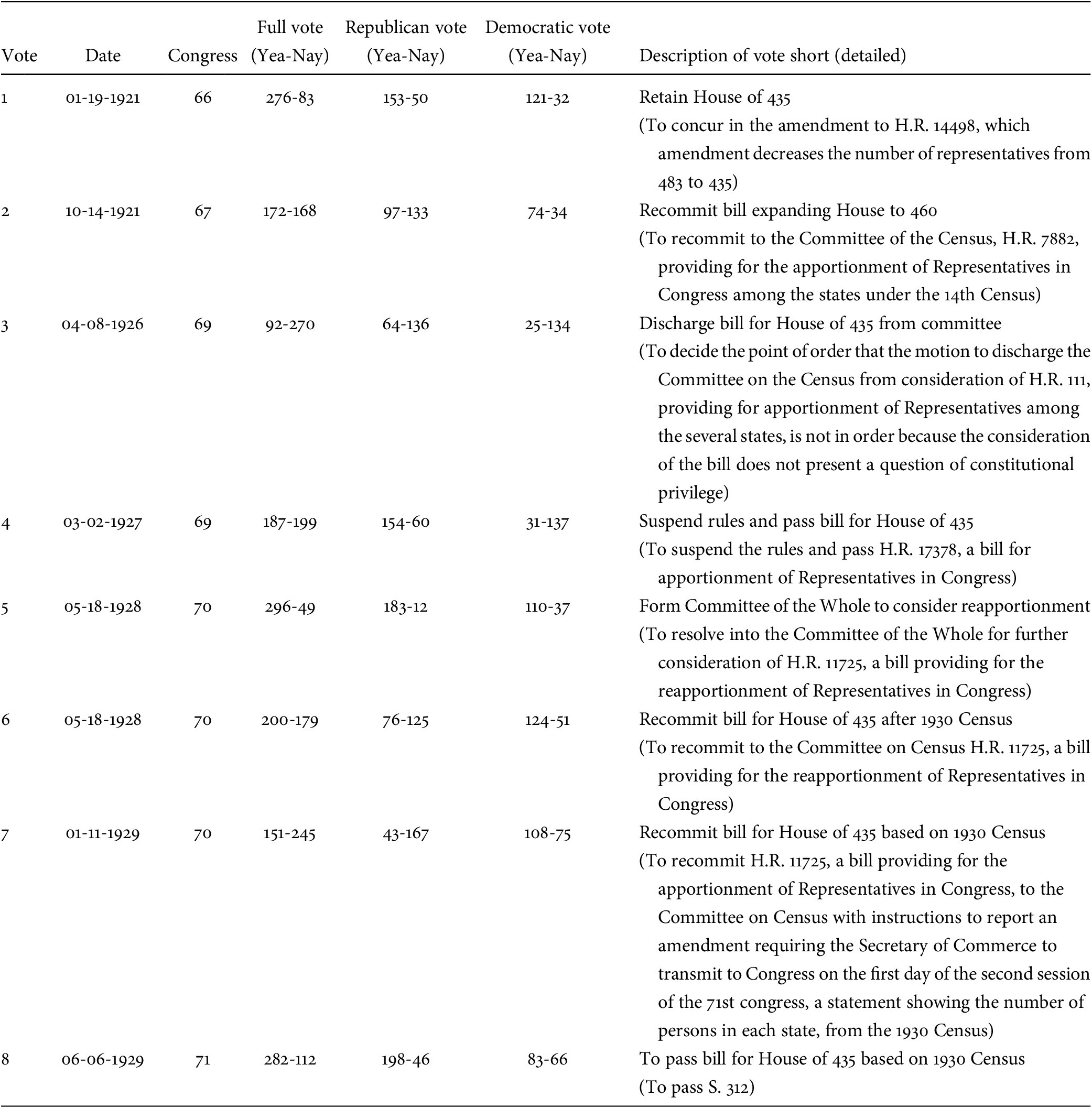
Source: Eagles, Democracy Delayed and voteview.com.
To test each hypothesis, we must measure each of the relevant concepts. The party hypothesis simply requires a binary variable for whether each member is a Republican or not. To test the conditional party government hypothesis, we incorporate NOMINATE scores—the standard measure of members’ ideological preferences based on aggregate data on how members of Congress voted throughout their careers—and compute the absolute difference between each member’s first-dimension NOMINATE score and that of their party’s median member such that larger numbers indicate more divergence between a member and their party’s median preference and smaller numbers indicate the opposite.Footnote 42 We expect members distant from their party medians not to support expanding the House (roll call number 2). For the lost seats hypothesis, we construct a binary variable that is equal to 1 if a member represents a district in a state slated to lose a seat under reapportionment and 0 otherwise; this variable is based on Eagles.Footnote 43 For the copartisan state legislature hypothesis, we collect data on the partisan composition of state legislatures from Michael J. Dubin’s reference book and construct a factor variable that takes on one of three values: Copartisan if both state legislative chambers were controlled by a majority of copartisan legislators, Divided Legislature if each chamber of the state legislature was controlled by different parties, or Contrapartisan if both state legislative chambers were controlled by a majority of contrapartisan legislators.Footnote 44 We expect that members with friendly state legislatures will be most likely to support the final bill that empowered state legislatures (roll call number 8). Next, for the urban–rural hypothesis, we measure the population density of each congressional district as the logged value of the population per square kilometer such that larger values represent urban districts and smaller ones represent rural ones. Finally, we also control for members’ prior voting behavior by including their first- and second-dimension NOMINATE scores and for the number of districts allocated to each state after the 1910 reapportionment.Footnote 45
To estimate the relationships between each of the preceding variables and a legislator’s decision to vote in favor of reapportionment, we employ multiple regression, a standard technique in empirical social science. Multiple regression allows us to examine how the probability of voting for or against reapportionment varies with our variables of interest while holding constant all other variables. Testing each hypothesis in isolation could lead to biased estimates of the effect of each variable if the variables are correlated. For example, if most members of Congress from states slated to gain seats also shared partisanship with their state’s legislature, then the effect of both gaining seats and sharing partisanship with one’s state legislature would be confounded. By using multiple regression, we can estimate the effect of each variable adjusting for the effect of each other—which is necessary when testing multiple hypotheses.Footnote 46
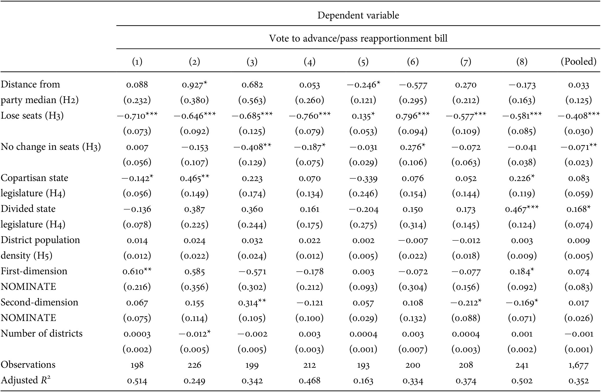
Specifically, we estimate nine models, one for each of the eight roll calls and one pooling all eight votes into a single model, using ordinary least squares regression. Table 2 reports the results. We find support for both the party hypothesis and the lost seats hypothesis. Republicans were significantly more likely to support reapportionment, and members from states slated to lose seats or stand pat were significantly less likely to support reapportionment when compared with those from states slated to gain seats. We find limited evidence that members from states with a divided state legislature were more likely to support reapportionment but that those from states with a copartisan state legislature were no more likely to support reapportionment than were those from states with a contrapartisan state legislature. We find no evidence that members from rural areas opposed reapportionment independent of other factors, such as party or ideology. Likewise, we find no evidence for the second hypothesis that ideological disagreement with a member’s party influenced whether they supported or opposed reapportionment.
Table 2. Roll-Call Analysis of Reapportionment Votes (all members)

Note: Unit of analysis is the member of Congress. Standard errors clustered by state in models 1–8 and by legislator in the pooled model. Pooled model includes roll-call fixed effects. Estimated via ordinary least squares. Contents of each vote can be found in Table 1; *p < 0.05, **p < 0.01, ***p < 0.001.
We then reestimate the models by party: Democratic results appear in Table 3; Republican results appear in Table 4. For Democrats, we only find consistent support for the lost seats hypothesis. For Republicans, we find results similar to those in the overall model. Republicans representing districts from states that would lose seats were about 41 percentage points less likely to support reapportionment than were those representing districts from states that would gain seats. And those Republicans representing states that would neither gain nor lose seats were about 8 percentage points less likely to support reapportionment compared with those representing states that would gain seats. We do, however, find some weak evidence that Republicans from states with Democratically controlled state legislatures, mostly from the South, were less likely to support reapportionment compared with Republican members representing states with a divided state legislature. But, in the aggregate we find no evidence that Republicans representing states with copartisan state-legislative majorities voted differently from those representing states with contrapartisan majorities in each chamber, but on the final passage vote for the bill to empower state legislatures, we did estimate effects in the expected direction.Footnote 47
Table 3. Roll-Call Analysis of Reapportionment Votes (Democrats Only)

Note: Unit of analysis is the member of Congress. Standard errors clustered by state in models 1–8 and by legislator in the pooled model. Pooled model includes roll-call fixed effects. Estimated via ordinary least squares. Contents of each vote can be found in Table 1; *p < 0.05, **p < 0.01, ***p < 0.001.
Table 4. Roll-Call Analysis of Reapportionment Votes (Republicans Only)
Note: Unit of analysis is the member of Congress. Standard errors clustered by state in models 1–8 and by legislator in the pooled model. Pooled model includes roll-call fixed effects. Estimated via ordinary least squares. Contents of each vote can be found in Table 1; *p < 0.05, **p < 0.01, ***p < 0.001.
Our approach allows us to better understand the final compromise in 1929 that broke the logjam. Introduced by Edward Hart Fenn (R-CT), the bill that eventually became law would delegate reapportionment to the Executive Branch and instruct the Department of Commerce to reapportion according to an automatic formula based upon population numbers from the forthcoming 1930 Census. However, the primary difference between this bill and other failed ones came when Fenn himself amended his own bill, striking section three, which had required that state legislatures draw districts “composed of contiguous and compact territory” that “contain as nearly as practicable the same number of individuals.”Footnote 48 These limitations on state power to redistrict had largely been in effect since the 1870s, and they would not return until a series of Supreme Court cases beginning in the 1960s.Footnote 49
Eagles called the move “inexplicable,” but the amendment gave hope to members from states that might lose seats or otherwise opposed reapportionment by empowering state legislatures to draw lines as they saw fit.Footnote 50 And it rewarded those members that had friendly state legislatures back home. In our analysis of Republican votes on this final bill (column 8), representatives from states with copartisan legislatures were 23 percentage points more likely to support the bill than were those from states with contrapartisan ones, and those from states with divided legislatures were 47 percentage points more likely to support the bill than were those from states with contrapartisan ones. In the end, 81 percent of Republicans voted for the bill, the largest proportion of any of the bills considered throughout the decade. The Fenn bill, and resulting Reapportionment and Census Act of 1929, moved the battle over congressional representation from a battle over apportionment in Congress to one over redistricting in the states, the ramifications of which are still felt today—as it empowered state legislatures to gerrymander much more so than they could have under previous laws passed in the early nineteenth century and during Reconstruction.Footnote 51
V Discussion and Conclusion
Although the rhetorical debates on the House floor in the 1920s were wide-ranging—with concerns about economy, demography, and political power—ultimately what mattered most on average for individual members’ votes to reapportion was their own political self-interest. Those from states slated to lose seats—and some members from states that could not trust their state legislatures to redistrict in their favor—were unlikely to support reapportionment. Partisanship mattered as well, with Republicans slightly more likely than Democrats to vote for reapportionment, which was understandable given that Republicans commanded a majority of seats in the chamber and on the committees and therefore controlled the agenda for the most part. Political self-interest still structures congressional behavior today, and thus similar voting patterns might result if Congress elects to retake control over apportionment by repealing the 1929 law. For example, states set to lose seats would likely prefer to expand the House. The urban–rural divide is also arguably more pronounced today;Footnote 52 thus, members representing rural districts with constituents who resent both increasing urbanization and the nation’s continued attempts to fully integrate racial, ethnic, and national minorities into the political process would likely reject any attempt to reapportion that would reallocate power to diverse urban centers. However, the two parties are more internally united than they were in the 1920s and may have the political capital and procedural tools to whip their members who oppose reapportionment to instead vote in favor if it would benefit the party as a whole.
Passage of the Apportionment and Census Act of 1929 was facilitated by empowering state legislatures to redistrict their apportioned seats as they saw fit, removing requirements of equal population, compactness, and contiguity that had been in effect since the 1870s and delegating power to state legislatures with few federal limitations. Beginning in the 1960s, however, the Supreme Court ruled that states could not disregard equal population, compactness, and contiguity when redistricting, removing the key provision that facilitated passage of the 1929 law. Additionally, several states have wrested authority over redistricting from state legislatures and given it to independent commissions.Footnote 53 Together, the Supreme Court’s rulings in the 1960s and the rise of independent redistricting commissions may threaten any contemporary compromise over apportionment because delegation to the states without limitations is unconstitutional and the effects of delegation to states with limitations may become increasingly unpredictable as states seek to remove power over redistricting from elected, partisan officials. Any successful revision of the apportionment process would require a new compromise from an extremely polarized Congress.


 Open access