

INTRODUCTION
Although there is strong evidence to suggest that large-scale environmental factors determine species distributions and community composition in tropical forests (Baldeck et al. Reference BALDECK, HARMS, YAVITT, JOHN, TURNER, VALENCIA, NAVARRETE, DAVIES, CHUYONG, KENFACK, THOMAS, MADAWALA, GUNATILLEKE, GUNATILLEKE, BUNYAVEJCHEWIN, KIRATIPRAYOON, YAACOB, SUPARDI and DALLING2013, Condit et al. Reference CONDIT, ENGELBRECHT, PINO, PÉREZ and TURNER2013, Harms et al. Reference HARMS, CONDIT and HUBBELL2001, John et al. Reference JOHN, DALLING, HARMS, YAVITT, STALLARD, MIRABELLO, HUBBELL, VALENCIA, NAVARRETE, VALLEJO and FOSTER2007), our knowledge of how the environment influences biomass at fine scales is limited. Landscape-scale studies in the tropics (Clark & Clark Reference CLARK and CLARK2000, Laurance et al. Reference LAURANCE, FEARNSIDE, LAURANCE, DELAMONICA, LOVEJOY, RANKIN-DE MERONA, CHAMBERS and GASCON1999) have focused on coarse variation in soil type and topography with conflicting results (Unger et al. Reference UNGER, HOMEIER and LEUSCHNER2012). The extent to which small-scale variation in soil nutrients and forest dynamics (Brienen et al. Reference BRIENEN, PHILLIPS, FELDPAUSCH, GLOOR, BAKER, LLOYD, LOPEZ-GONZALEZ, MONTEAGUDO-MENDOZA, MALHI, LEWIS, VASQUEZ MARTINEZ, ALEXIADES, ALVAREZ DAVILA, ALVAREZ-LOAYZA, ANDRADE, ARAGAO, ARAUJO-MURAKAMI, ARETS, ARROYO and AYMARD2015) affect biomass in tropical forests is an open question. However, it is vital to know this for understanding carbon source/sink dynamics (Phillips et al. Reference PHILLIPS, MALHI, HIGUCHI, LAURANCE, NÚÑEZ, VÁSQUEZ, LAURANCE, FERREIRA, STERN, BROWN and GRACE1998, Wright Reference WRIGHT2005) and estimating global carbon reservoirs (Dixon et al. Reference DIXON, SOLOMON, BROWN, HOUGHTON, TREXIER and WISNIEWSKI1994, Schimel Reference SCHIMEL1995). At the same time, it is important to consider that the notion of an untouched, monolithic primeval rain forest is being reconsidered (Clark Reference CLARK1996, Whitmore Reference WHITMORE1990, Reference WHITMORE, Gomez-Pompa, Whitmore and Hadley1991) as the long and varied history of natural and anthropogenic disturbance across the tropics continues to be documented (Chazdon Reference CHAZDON2003, Reference CHAZDON2014). These variations are often correlated with species’ life-history strategies (Wright et al. Reference WRIGHT, KITAJIMA, KRAFT, REICH, WRIGHT, BUNKER, CONDIT, DALLING, DAVIES, DIAZ, ENGELBRECHT, HARMS, HUBBELL, MARKS, RUIZ-JAEN, SALVADOR and ZANNE2010), global patterns of productivity (Stephenson & Mantgem Reference STEPHENSON and MANTGEM2005), carbon storage (Doughty et al. Reference DOUGHTY, METCALFE, GIRARDIN, AMEZQUITA, CABRERA, HUASCO, SILVA-ESPEJO, ARAUJO-MURAKAMI, DA COSTA, ROCHA, FELDPAUSCH, MENDOZA, DA COSTA, MEIR, PHILLIPS and MALHI2015) and the maintenance of species diversity (Connell Reference CONNELL1978, Molino & Sabatier Reference MOLINO and SABATIER2001).
Previous studies of forest regeneration (Brown & Lugo Reference BROWN and LUGO1990, Chazdon Reference CHAZDON2014, Lebrija-Trejos et al. Reference LEBRIJA-TREJOS, BONGERS, PÉREZ-GARCÍA and MEAVE2008, Letcher Reference LETCHER2010) in forest plots at least 0.1 ha in size have documented changes in species richness, trait diversity, phylogenetic diversity and basal area in a variety of tropical forests. Few such studies have accounted for small-scale species interactions in mature forests, although remote-sensing (Chambers et al. Reference CHAMBERS, NEGRON-JUAREZ, MARRA, DI VITTORIO, TEWS, ROBERTS, RIBEIRO, TRUMBORE and HIGUCHI2013) and natural history approaches (Martinez-Ramos et al. Reference MARTINEZ-RAMOS, ALVAREZ-BUYLLA, SARUKHAN and PINERO1988) have been used to date small canopy gaps and forest disturbance rates.
One region that still contains an almost continuous landscape of lowland rain forest (Mittermeier et al. Reference MITTERMEIER, MYERS, THOMSEN, DA FONSECA and OLIVIERI1998) but remains understudied (Whitfeld et al. Reference WHITFELD, KRESS, ERICKSON and WEIBLEN2012, Reference WHITFELD, LASKY, DAMAS, SOSANIKA, MOLEM and MONTGOMERY2014) is the island of New Guinea. What makes this area noteworthy is a geological legacy of more than 3 million y of unusually high tectonic surface uplift following collision of the Finisterre Volcanic arc terrane and the Australian continental margin (Abbott et al. Reference ABBOTT, SILVER, ANDERSON, SMITH, INGLE, KLING, HAIG, SMALL, GALEWSKY and SLITER1997). As a result, the soils are geologically young, unstable and nutrient-rich (Loffler Reference LOFFLER1977). It has been suggested that forests on the island are unusually dynamic and less productive than other lowland rain forests (Garwood et al. Reference GARWOOD, JANOS and BROKAW1979, Johns Reference JOHNS1986, Vincent et al. Reference VINCENT, HENNING, SAULEI, SOSANIKA and WEIBLEN2015) but there is limited quantitative documentation of this prediction. Here we used partial re-census data from a long-term forest dynamics plot in New Guinea to investigate small-scale (20 × 20 m) forest dynamics (tree recruitment, growth and mortality), disturbance, forest age and the influence of the abiotic environment on species composition and basal area. In addition, we incorporated topography, soil nutrients and a dated chronosequence to identify possible ecological processes affecting lowland New Guinea rain forests. If New Guinea's forests are, indeed, highly dynamic we hypothesize: no association of soil nutrients and fine-scale topographic variation with (1) basal area distributions and (2) species composition, (3) no spatial structure in age-class distributions and (4) higher mortality and an overall younger forest compared with other tropical regions. Where possible, we present parallel analyses from a neotropical plot on Barro Colorado Island (BCI), Panama and also comparisons with other tropical forests to contextualize our study.
STUDY SITE
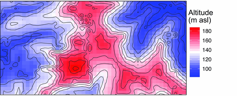
The 50-ha Wanang forest dynamics plot (FDP), part of the Center for Tropical Forest Science Global Earth Observatory (CTFS-ForestGEO) global network of forest plots (Anderson-Teixeira et al. Reference ANDERSON-TEIXEIRA, DAVIES, BENNETT, GONZALEZ-AKRE, MULLER-LANDAU, JOSEPH WRIGHT, ABU SALIM, ALMEYDA ZAMBRANO, ALONSO, BALTZER, BASSET, BOURG, BROADBENT, BROCKELMAN, BUNYAVEJCHEWIN, BURSLEM, BUTT, CAO, CARDENAS and CHUYONG2015), is located in mature lowland rain forest in Madang province in northern Papua New Guinea (Vincent et al. Reference VINCENT, HENNING, SAULEI, SOSANIKA and WEIBLEN2015). The FDP is situated in a nearly contiguous block of forest comprising 18.5 million ha (Shearman et al. Reference SHEARMAN, ASH, MACKEY, BRYAN and LOKES2009). Soils at Wanang are a heterogeneous mixture of Entisols, Inceptisols and Alfisols, depending on the timing of disturbance and exposure of parent material (Turner et al. unpubl. data). Rainfall averages 4000 mm annually, with no month receiving <125 mm. There is significant topographical relief in the plot, with riparian areas (~90 m asl) flanking both short ends of the rectangular FDP (500 × 1000 m) and a large, steep-sided main ridge bisecting the plot north to south (~190 m asl) (Figure 1). This landscape of Pliocene and Pleistocene mudstone is typical for lowland forest areas in northern New Guinea.

Figure 1. Mean altitude per quadrat in the Wanang forest dynamics plot, Papua New Guinea, is represented by a colour gradient from blue (lowest) to red (highest). Contour lines show topographical relief in the plot corresponding to variation in altitude represented in the coloured quadrat boxes.
METHODS
Plot census
The Wanang FDP was established in 2009 following protocols developed by CTFS-ForestGEO (Condit Reference CONDIT1995, Reference CONDIT1997). The plot was gridded to 10 cm accuracy into 1250 quadrats, each 20 m by 20 m. An intensive topographical survey was conducted during plot establishment and elevation readings were taken at the corner of each quadrat. From these values, indices of mean elevation (average elevation of the four corners of each quadrat), slope (average slope of four planes created by connecting three corners of each quadrat at a time), and convexity (mean elevation of the focal quadrat minus the average elevation of all directly adjacent quadrats) were determined per quadrat (Harms et al. Reference HARMS, CONDIT and HUBBELL2001).
During plot enumeration, every stem ≥1 cm in diameter at breast height was tagged, measured, mapped (±10 cm), and identified to species or morphospecies, often based on sterile individuals and comparison of voucher specimens to already identified herbarium collections. Collection of voucher specimens for all taxa is ongoing. These specimens are deposited in the Papua New Guinea Forest Research Institute Herbarium (LAE) and the Bell Museum Herbarium at the University of Minnesota (MIN). The first census recorded a total of 290,012 stems belonging to 267,951 individual trees comprising 580 taxa, including 528 species and 52 morphospecies in 259 genera and 84 families.
Basal area
Basal area (BA) was calculated from diameter at breast height measurements, assuming circular stems, summed per 20 × 20-m quadrat. This process was repeated using available data from BCI, one of the oldest plots in the CTFS-ForestGEO network of plots. We tested for a difference in distributions of basal area per quadrat between the BCI and Wanang FDPs using a Wilcoxon rank-sum test, as basal area distributions violated the assumption of normality even after attempts to transform the data. Basal area values per quadrat were also used to create a map of basal area distribution in the Wanang FDP. We used basal area as a proxy for above-ground biomass since measurements of trunk height and wood specific gravity (necessary for estimating biomass) were not available for all species at our study site.
Soil analysis and interpolation
Soils were collected at 296 locations in the Wanang 50-ha plot between April and May 2013 using a sampling protocol described previously (Baldeck et al. Reference BALDECK, HARMS, YAVITT, JOHN, TURNER, VALENCIA, NAVARRETE, DAVIES, CHUYONG, KENFACK, THOMAS, MADAWALA, GUNATILLEKE, GUNATILLEKE, BUNYAVEJCHEWIN, KIRATIPRAYOON, YAACOB, SUPARDI and DALLING2013, John et al. Reference JOHN, DALLING, HARMS, YAVITT, STALLARD, MIRABELLO, HUBBELL, VALENCIA, NAVARRETE, VALLEJO and FOSTER2007). At each sampling point, five cores were taken to 10 cm with a 2.54 cm diameter corer and combined into a single composite sample. Samples were air dried, sieved <2 mm. Soil pH was determined in both deionized water and 10 mM CaCl2 in a 1:2 soil to solution ratio using a glass electrode. Concentrations of Al, Ca, Fe, K, Mg, Mn and Na were determined by extraction in 0.1 m BaCl2 (2 h, 1:30 soil to solution ratio), with detection by inductively coupled plasma optical-emission spectrometry (ICP–OES) on an Optima 7300 DV (Perkin-Elmer Ltd, Shelton, CT) (Hendershot et al. Reference HENDERSHOT, LALANDE, DUQUETTE, Carter and Gregorich2008). Nitrogen mineralization was determined using in-field ion-exchange resins at the same sites as soil collection during April and May of 2013. Five grams of mixed-bed ion-exchange resin (Dowex Marathon Mr-3) was enclosed within a 6 × 7.5-cm mesh bag (polyester monofilament, 220 micron mesh opening) sewn with monofilament thread. Bags were inserted into the upper mineral soil horizon at a 45° angle by making a cut with a machete, inserting the bag, and gently tamping the surface to enclose the bag in the soil. All bags except three were retrieved after approximately 3 wk in the field. The bags were rinsed thoroughly in deionized water and then nutrients were extracted with 75 mL of 0.5 m HCl for simultaneous determination of ammonium, nitrate and phosphate in neutralized extracts by automated colorimetry on a Lachat QuikChem 8500 (Hach Ltd, Loveland, CO). Ammonium and nitrate concentrations are a time-integrated measure of nitrogen mineralization during the study period whereas we interpreted phosphate concentrations as reflecting a dynamic equilibrium between the resin and the soil.
All soil nutrients were block-kriged following John et al. (Reference JOHN, DALLING, HARMS, YAVITT, STALLARD, MIRABELLO, HUBBELL, VALENCIA, NAVARRETE, VALLEJO and FOSTER2007). We interpolated measured values while incorporating spatial variation depicted in variogram models to produce estimates of nutrient concentrations per quadrat. In the kriging procedure, variogram fits for Ca and K were manually adjusted to better capture broad-scale trends in soil nutrient variation by reducing the effect of unusually high variation at small spatial scales. Aggregate measures of total exchangeable bases (TEB), exchangeable cation concentration (ECEC), and base saturation (BS) were calculated after kriging as follows: TEB was calculated as the sum of the charge equivalents of Ca, K, Mg and Na; ECEC was calculated as the sum of the charge equivalents of Al, Ca, Fe, K, Mg, Mn and Na; BS was calculated as (TEB ÷ ECEC) × 100.
Plot re-census
Fifty-two randomly selected quadrats (2.08 ha total) in the Wanang FDP were re-censused. Each tree was relocated and its diameter at breast height re-measured if living or marked as dead. An individual tree may have multiple stems that branch below 1.3 m, herein our recruitment and mortality results refer to analyses using measurements of primary stems of individual trees and RGR refers to all stems. Relative growth rate (RGR) was estimated for each quadrat (RGRstand) and for all species (RGRspecies). RGR per quadrat was estimated as:
 $$\begin{equation*}
{\rm{RG}}{{\rm{R}}_{{\rm{stand}}}} = \left[ {{\rm{ln}}\,\left( {{\rm{B}}{{\rm{A}}_{\rm{t}}}} \right)-{\rm{ln}}\,\left( {{\rm{BA}}} \right)} \right]/{{\rm{t}}_{{\rm{quadrat}}}}
\end{equation*}$$
$$\begin{equation*}
{\rm{RG}}{{\rm{R}}_{{\rm{stand}}}} = \left[ {{\rm{ln}}\,\left( {{\rm{B}}{{\rm{A}}_{\rm{t}}}} \right)-{\rm{ln}}\,\left( {{\rm{BA}}} \right)} \right]/{{\rm{t}}_{{\rm{quadrat}}}}
\end{equation*}$$
Where BAt and BA, are basal area of all stems at the time of re-census and initial census respectively, and tquadrat is the re-census interval in years for the focal quadrat.
RGR was estimated for all species as:
 $$\begin{equation*}
{\rm{RG}}{{\rm{R}}_{{\rm{species}}}} = \left[ {{\rm{ln}}\,\left( {{\rm{B}}{{\rm{A}}_{\rm{t}}}} \right)-{\rm{ln}}\,\left( {{\rm{BA}}} \right)} \right]/{{\rm{t}}_{{\rm{avg}}}}
\end{equation*}$$
$$\begin{equation*}
{\rm{RG}}{{\rm{R}}_{{\rm{species}}}} = \left[ {{\rm{ln}}\,\left( {{\rm{B}}{{\rm{A}}_{\rm{t}}}} \right)-{\rm{ln}}\,\left( {{\rm{BA}}} \right)} \right]/{{\rm{t}}_{{\rm{avg}}}}
\end{equation*}$$
Where BAt and BA are basal area of all stems at the time of re-census and initial census respectively, and tavg is the average census interval for all quadrats. Average census interval was used in estimation of species-level growth rate as stems belonging to each species were distributed across many quadrats with different re-census intervals.
Recruitment rate (r) was estimated for the entire tree community as:
 $$\begin{equation*}
{\rm{r}} = \left[ {{\rm{ln}}\left( {\rm{R}} \right)-{\rm{ln}}\left( {{\rm{R}}^{*}} \right)} \right]/{{\rm{t}}_{{\rm{avg}}}}
\end{equation*}$$
$$\begin{equation*}
{\rm{r}} = \left[ {{\rm{ln}}\left( {\rm{R}} \right)-{\rm{ln}}\left( {{\rm{R}}^{*}} \right)} \right]/{{\rm{t}}_{{\rm{avg}}}}
\end{equation*}$$
Where R* is the number of individuals alive in both censuses, R is R* plus new recruits, and tavg is the average census interval in years.
Our estimate of annual mortality was calculated using a common measure of mortality in forests (Clark & Clark Reference CLARK and CLARK1992, Condit et al. Reference CONDIT, HUBBELL and FOSTER1995, Phillips et al. Reference PHILLIPS, HALL, GENTRY, SAWYER and VÁSQUEZ1994):
 $$\begin{equation*}
{\rm{m}} = \left[ {{\rm{ln}}\left( {{{\rm{N}}_0}} \right)-{\rm{ln}}\left( {{{\rm{N}}_{\rm{t}}}} \right)} \right]/{{\rm{t}}_{{\rm{avg}}}}
\end{equation*}$$
$$\begin{equation*}
{\rm{m}} = \left[ {{\rm{ln}}\left( {{{\rm{N}}_0}} \right)-{\rm{ln}}\left( {{{\rm{N}}_{\rm{t}}}} \right)} \right]/{{\rm{t}}_{{\rm{avg}}}}
\end{equation*}$$
Where N0 is the number of individuals at the time of the initial census, Nt is the number of individuals surviving at re-census, and tavg is the average time (y) between censuses.
We compiled published mortality estimates (only those including all trees ≥1 cm) from tropical rain forests worldwide for comparison with New Guinea. Considering the small size of our re-census dataset (2.08 ha), we were unable to calculate rates for different size classes (e.g. ≥10 cm diameter) or groups of edaphic specialists (Russo et al. Reference RUSSO, DAVIES, KING and TAN2005) or habitat specialists (Chisholm et al. Reference CHISHOLM, CONDIT, RAHMAN, BAKER, BUNYAVEJCHEWIN, CHEN, CHUYONG, DATTARAJA, DAVIES, EWANGO, GUNATILLEKE, NIMAL GUNATILLEKE, HUBBELL, KENFACK, KIRATIPRAYOON, LIN, MAKANA, PONGPATTANANURAK, PULLA and PUNCHI-MANAGE2014). We therefore focused our comparison on measures of overall mortality rate, regardless of species or size class (Condit et al. Reference CONDIT, HUBBELL and FOSTER1995, Reference CONDIT, ASHTON, MANOKARAN, LAFRANKIE, HUBBELL and FOSTER1999; Shen et al. Reference SHEN, SANTIAGO, MA, LIN, LIAN, CAO and YE2013).
Statistical analyses
Spatial variation in species composition was visualized following Baldeck et al. (Reference BALDECK, HARMS, YAVITT, JOHN, TURNER, VALENCIA, NAVARRETE, DAVIES, CHUYONG, KENFACK, THOMAS, MADAWALA, GUNATILLEKE, GUNATILLEKE, BUNYAVEJCHEWIN, KIRATIPRAYOON, YAACOB, SUPARDI and DALLING2013). A community matrix of individuals per species by quadrat was created for the Wanang FDP. This matrix was converted into a Bray–Curtis dissimilarity matrix (Bray & Curtis Reference BRAY and CURTIS1957), a popular quantitative dissimilarity measure, which was used in a three-dimensional non-metric multidimensional scaling (NMDS) ordination using the function ‘metaMDS’ from the vegan package for R. The position of each quadrat in three-dimensional ordination space reflects their similarity in species composition. These positions were scaled between zero and 1 using maximum and minimum values in each direction and then translated into RGB colours by assigning each quadrat's position on the first three ordination axes to intensities of red, green and blue (Thessler et al. Reference THESSLER, RUOKOLAINEN, TUOMISTO and TOMPPO2005). The translation of colour intensity was applied to all axes simultaneously such that colour variation reflects variation explained by the respective axes. RGB components of each quadrat were combined to create composite colour values that were subsequently mapped for each quadrat (Baldeck et al. Reference BALDECK, HARMS, YAVITT, JOHN, TURNER, VALENCIA, NAVARRETE, DAVIES, CHUYONG, KENFACK, THOMAS, MADAWALA, GUNATILLEKE, GUNATILLEKE, BUNYAVEJCHEWIN, KIRATIPRAYOON, YAACOB, SUPARDI and DALLING2013) to produce a coloured visualization of local variation in community composition (Anderson et al. Reference ANDERSON, CRIST, CHASE, VELLEND, INOUYE, FREESTONE, SANDERS, CORNELL, COMITA, DAVIES, HARRISON, KRAFT, STEGEN and SWENSON2010).
Variance partitioning (Borcard et al. Reference BORCARD, LEGENDRE and DRAPEAU1992) by redundancy analysis (RDA) in the case of multivariate data for community composition and partial regression for basal area per quadrat was performed to evaluate associations of topography, soil nutrients and spatial proximity with species composition and basal area distributions. Function ‘varpart’ from the vegan package in R was used with the response variables being either a community matrix of quadrats by species or basal area per quadrat and explanatory matrices being topographic variables and soil nutrients. Principal coordinates of neighbourhoods matrix (PCNM) (Borcard & Legendre Reference BORCARD and LEGENDRE2002, Dray et al. Reference DRAY, LEGENDRE and PERES-NETO2006) was used to account for the possible influence of spatial autocorrelation (Legendre et al. Reference LEGENDRE, BORCARD and PERES-NETO2005, Reference LEGENDRE, MI, REN, MA, YU, SUN and HE2009), using the function ‘pcnm’ from the vegan package in R. The method uses a truncated Euclidean distance matrix of neighbouring quadrats defined as those directly adjacent, including diagonals (i.e. Queen's criterion), for a maximum of eight neighbours per quadrat. The distance of all neighbouring quadrats is maintained and all non-neighbour distances are then set to four times the distance between points following Borcard & Legendre (Reference BORCARD and LEGENDRE2002). All positive eigenvalues of a principal coordinates analysis (PCoA) on the truncated distance matrix are maintained for inclusion in ordination or regression analyses to account for the effect of spatial proximity of samples in the variance-partitioning procedure. Adjusted r2 values are derived for each testable fraction of explanatory factors following Peres-Neto et al. (Reference PERES-NETO, LEGENDRE, DRAY and BORCARD2006), providing a robust estimate of variation explained while adjusting for the number of explanatory variables. Similar partitioning procedures have been used to investigate the influence of spatial structure and abiotic variables on species composition of tropical and subtropical forests (Baldeck et al. Reference BALDECK, HARMS, YAVITT, JOHN, TURNER, VALENCIA, NAVARRETE, DAVIES, CHUYONG, KENFACK, THOMAS, MADAWALA, GUNATILLEKE, GUNATILLEKE, BUNYAVEJCHEWIN, KIRATIPRAYOON, YAACOB, SUPARDI and DALLING2013, Legendre et al. Reference LEGENDRE, MI, REN, MA, YU, SUN and HE2009). A schematic Venn-diagram showing variance partitioning components and labelling conventions is included (Figure 2).
Figure 2. Components of variance-partitioning analysis for species composition and basal area per quadrat in the Wanang forest dynamics plot, Papua New Guinea depicted as a Venn diagram. Letter labels correspond to elements of each tested component of variation as presented in Table 1. Each circle in the Venn diagram represents a different set of explanatory variables, overlapping areas represent components shared between explanatory variables. ‘Topography’ represents variance explained by topographical indices of mean elevation, slope and convexity per quadrat. ‘Soils’ represents variation explained by a matrix of soil nutrient variables per quadrat. ‘Spatial’ represents variation explained by positive eigenvectors from the PCNM analysis, indicative of spatial structure in the response data. ‘Residuals’ represents the portion of variance not accounted for in the variance partitioning among our three explanatory matrices.
Regeneration phase
Stem size class ratios have been used in the past to account for regenerative character or gap-phase (GP) dynamics (Feeley et al. Reference FEELEY, DAVIES, ASHTON, BUNYAVEJCHEWIN, NUR SUPARDI, KASSIM, TAN and CHAVE2007) in analyses of forest inventory data. We calculated an index of forest regeneration phase following Feeley et al. (Reference FEELEY, DAVIES, ASHTON, BUNYAVEJCHEWIN, NUR SUPARDI, KASSIM, TAN and CHAVE2007) to explore whether the signature of forest regeneration based on the log ratio of basal area held in large to small stems is similar in the New Guinea forest compared with other lowland rain forests for which we were able to obtain data. This gap phase (GP) statistic was calculated as:
 $$\begin{equation*}
{\rm{GP}} = {\rm{ln}}\left( {{\rm{B}}{{\rm{A}}_{30}} + 1} \right)-{\rm{ln}}\left( {{\rm{B}}{{\rm{A}}_{10}} + 1} \right)
\end{equation*}$$
$$\begin{equation*}
{\rm{GP}} = {\rm{ln}}\left( {{\rm{B}}{{\rm{A}}_{30}} + 1} \right)-{\rm{ln}}\left( {{\rm{B}}{{\rm{A}}_{10}} + 1} \right)
\end{equation*}$$
Where BA30 is the basal area in the focal quadrat held in stems 30 cm or larger and BA10 (m2 ha−1) is basal area held in stems less than 10 cm diameter at breast height. This measure is contingent on the assumption that the predominant fraction of basal area in forests proceeding through succession will shift from small stems to large stems, an established process in forest regeneration (Chazdon Reference CHAZDON, Carson and Schnitzer2008, Franklin et al. Reference FRANKLIN, SPIES, PELT, CAREY, THORNBURGH, BERG, LINDENMAYER, HARMON, KEETON, SHAW, BIBLE and CHEN2002). This transition will yield gap phase statistics differentiating more recently disturbed quadrats dominated by small stems (low GP) from older quadrats with an increased presence of large trees (high GP). This calculation was carried out for both Wanang and BCI and plotted as histograms and cumulative density curves of GP value per quadrat, coloured by plot. As in our comparison of basal area between BCI and Wanang, we tested for a difference in distributions of GP per quadrat using a Wilcoxon rank-sum test.
Chronosequence dating
Previous work close to the Wanang FDP established a set of 19 0.25-ha satellite plots (4.75-ha total) ranging from 3 to >50 y since disturbance to examine forest succession (Whitfeld et al. Reference WHITFELD, KRESS, ERICKSON and WEIBLEN2012, Reference WHITFELD, LASKY, DAMAS, SOSANIKA, MOLEM and MONTGOMERY2014). Forest age estimates in these plots combined evidence from forest-cover maps based on aerial photography and local community knowledge. In the present study, we used mean and standard deviation basal area measurements for each class of younger secondary (3–9 y old), older secondary (10–30 y old), intermediate mature (31–50 y old) and mature forest plots (>50 y old) (Whitfeld et al. Reference WHITFELD, LASKY, DAMAS, SOSANIKA, MOLEM and MONTGOMERY2014) to divide quadrats in the Wanang FDP plot to corresponding age class bins. We tested for correlation between age class distributions of the entire plot and the subset of re-censused quadrats.
The Indicspecies R package and function ‘multipatt’ (De Cáceres et al. Reference DE CÁCERES, LEGENDRE and MORETTI2010) was used to investigate similarity in species occurrence between quadrats of the 50-ha plot dated by basal area and the 0.25-ha satellite plots used for forest age dating. Indicator species were prioritized based on indicator value (Dufrêne & Legendre Reference DUFRÊNE and LEGENDRE1997), an index of fidelity and abundance in habitat types, and tested for statistical significance with 999 permutations of the community matrix. Only indicator species for a single age class were considered since we were attempting to match established age class categories rather than investigate species-habitat associations. Significant indicator species for different successional stages were compared with published results and analyses reproduced following Whitfeld et al. (Reference WHITFELD, LASKY, DAMAS, SOSANIKA, MOLEM and MONTGOMERY2014) to validate our plot dating method. Results of a detrended correspondence analysis (DCA) as well as importance values (IV) and dominance measures of chronosequence species were used for validation. Although there was a difference in species richness between the more extensively sampled 50-ha forest inventory plot and the chronosequence plots (581 total species versus 260 total species) the co-occurrence of species shown to indicate different successional stages suggests that portions of the 50-ha plot were in concurrent stages of forest regeneration with the dated satellite chronosequence plots.
RESULTS
Soil pH was relatively high (range 5.5–7.1 measured in water, mean 6.3±0.3) and soils contained abundant base cations (total exchangeable bases 20.4–69.9 cmolc kg−1, mean 37.3±6.6) and a wide range of available phosphate concentrations (0.8 to 35.8 mg P kg−1, mean 6.0±5.6). However, nitrate mineralization was relatively low compared with other sites in South-East Asia (mean nitrate 7.8 µg N per bag per day), presumably reflecting the relatively low rates of nitrogen emissions and atmospheric nitrogen deposition in the region (Hietz et al. Reference HIETZ, TURNER, WANEK, RICHTER, NOCK and WRIGHT2011).
Combined soil, topographical and spatial variables were statistically associated with 29% of variation in community composition in the Wanang plot (Table 1, Figure 2). Individual fractions had much less explanatory power, soil alone explaining 6% of variation and topography 8%. The variation in species composition across the FDP can be visualized in the map of local variation in community composition produced by translating coordinates from three-dimensional NMDS into RGB colours (Figure 3a).
Table 1. Variance partitioning results for species composition and basal area per quadrat in the Wanang forest dynamics plot, Papua New Guinea. Following Baldeck et al. (Reference BALDECK, HARMS, YAVITT, JOHN, TURNER, VALENCIA, NAVARRETE, DAVIES, CHUYONG, KENFACK, THOMAS, MADAWALA, GUNATILLEKE, GUNATILLEKE, BUNYAVEJCHEWIN, KIRATIPRAYOON, YAACOB, SUPARDI and DALLING2013) lettered variance components are labelled with reference to Figure 2: total – overall proportion of variation explained by all variables combined (a + b + c + d + e + f + g), spatial – variation explained by spatial variables (a+d+f+g), environment – variation explained by soils and topography (b+c+d+e+f+g), spatial|environment – variation explained by spatial variables while controlling for soils and topographical variables (a), spatial & environment – spatially structured variation in topographical soil variables (d+f+g), environment|spatial –variation explained by topography and soils while controlling for spatial structure (b+c+e), soils – proportion of variation explained by soil nutrients (b+d+e+g), topography –variation explained by topographical variables (c+e+f+g), soils|topography – variation explained by soil variables while controlling for topographical variables (c+d), soils & topography –variation explained by topographically structured variation in soil nutrients (e+g), topography|soils – variation explained by topography after controlling for soil variables (c+f). Values are adjusted r2 values, a robust estimator of variance explained that adjusts for the number of variables in the model.
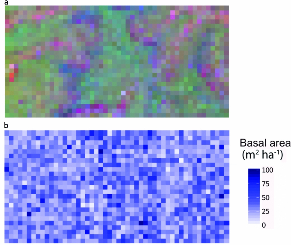
Figure 3. Spatial distribution of tree species composition and basal area in the Wanang forest dynamics plot, Papua New Guinea. Each individual square corresponds to a 20 × 20-m quadrat. Quadrats are coloured as determined by locations in a three-dimensional non-metric multidimensional scaling space, based on species composition (a) and basal area values per quadrat (b).
Soil, topography and spatial variables, whether considered solely or in aggregate, explained little variation in basal area (4%) (Table 1). No patterns corresponding to coarse topography (e.g. mean elevation, Figure 1) were apparent, nor does basal area appear to be spatially structured in other ways (Figure 3b).
Average basal area per quadrat in Wanang was 32.0±13.7 m2 ha−1, ranging from 2.73 to 104 m2 ha−1 (Figures 3b, 4). Basal area in the BCI FDP averaged 31.5±18.0 m2 ha−1 with a range of 8.18–167 m2 ha−1 (Figure 4). Results from a Wilcoxon rank-sum test suggested distributions of basal area per quadrat at the two sites were significantly different (P <0.001), likely based on a difference in shape primarily due to the presence of a long tail of high basal area quadrats at BCI.

Figure 4. Dot plot of basal area (m2 ha−1) per 20 × 20-m quadrat in the Wanang, Papua New Guinea, and Barro Colorado Island (BCI), Panama, forest dynamic plots. Overlapping data points were randomly jittered to either side of their true value to more clearly represent their density. Violin plots further illustrate the true cumulative density of data points within a sliding window.
Re-measurement of 52 quadrats (2.08 ha) resulted in data collection on 11139 individual trees with a total of 12153 stems belonging to 351 species. The interval between initial and second measurement ranged from 725 to 1313 d, with a mean and SD of 943±179 d (2.58±0.49 y). Annual mortality rate was estimated to be 3.95% (Table 2) and recruitment rate was estimated as 2.77% annually.
Table 2. Mortality rates of stems greater than or equal to 1 cm diameter at breast height in the present study and previously published literature. All studies referenced used the same equation to calculate estimates of mortality based on all individuals in respective plots. The four values for BCI, from Condit et al. (Reference CONDIT, HUBBELL and FOSTER1995, Reference CONDIT, ASHTON, MANOKARAN, LAFRANKIE, HUBBELL and FOSTER1999) and Shen et al. (Reference SHEN, SANTIAGO, MA, LIN, LIAN, CAO and YE2013) were averaged and reported with SD.

RGR was calculated on all stems showing diameter growth >0 cm, which corresponded to 9994 total stems. Plot-level RGR averaged 0.055±0.032 and ranged from 0.019 to 0.170. Values for the 12 species with 100 or more stems included in the re-census are presented in Table 3. Estimates of species-level growth rates (expressed as a percentage) averaged 6.1%, ranging from 2.1% in Aglaia lepiorrhachis to 15% in Ficus hahliana.
Table 3. Relative growth rates (RGR) for 12 species for which 100 or more stems were re-measured in the Wanang FDP, Papua New Guinea. Species are listed in order of decreasing number of stems measured. Estimates for RGRspecies were calculated using average census interval for all re-measured quadrats and expressed as percentage increases.
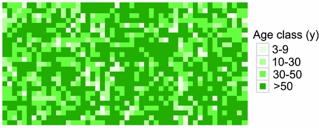
Dating quadrats in the Wanang FDP based on total basal area suggested that the majority of the FDP (671 quadrats, 55% plot) had not been disturbed in at least 50 y (Table 4). The next largest portion corresponded to forest aged 30–50 y old (27%). The 10–30- and <9-y areas accounted for 12% and 6% of the plot, respectively (Table 4). Mapping the distribution of these age classes showed no obvious correspondence to major topographical features (Figure 5). Age class distributions of the entire plot and re-census quadrats were highly correlated (r = 0.997).
Table 4. Forest-age classification criteria, age-class composition and average ± SD gap phase (GP) value per age class in the Wanang 50-ha plot, Papua New Guinea. GP values vary from low to high where plots are dominated by small or large stems respectively. All 20 × 20-m quadrats (n = 1250) in the plot were assigned to an age class defined by basal area as calculated from a series of dated 0.25-ha satellite plots.


Figure 5. Spatial distribution of age class categories in the Wanang forest dynamics plot, Papua New Guinea. Different age classes are represented on a scale of light to dark green showing younger to older age classes. Each square corresponds to one 20 × 20-m quadrat. Age classes were defined in Whitfeld et al. (Reference WHITFELD, LASKY, DAMAS, SOSANIKA, MOLEM and MONTGOMERY2014) based on a chronosequence of dated plots located near the Wanang FDP (Table 3).
Results of GP per quadrat for Wanang and BCI show highly overlapping distributions (Figure 6). Although distributions are similar for Wanang and BCI (Wilcoxon rank-sum test, P >0.05), the range of values are offset such that the Wanang FDP had GP values more negative GP values than BCI, and BCI had higher values than Wanang.

Figure 6. Values of gap phase (GP) per quadrat for forest dynamics plots in Wanang, Papua New Guinea, and Barro Colorado Island, Panama. Points were randomly adjusted to minimize over plotting and violin plots included to reflect cumulative density of values. GP values vary from low to high where plots are dominated by small or large stems respectively.
Measurements of GP by quadrat coloured by age class show that age class corresponds roughly to GP (Figure 7) and mean GP value per age class reflects differences in age class (Table 4). Younger forest quadrats had lower GP values than older quadrats, although there was considerable variation in GP value per age class (Table 4). For example, quadrats of the 10–30-y age class had an average (mean ± SD) GP value of 0.13±0.86 whereas quadrats in the 30–50-y age class averaged 0.65±0.58 (Table 4).
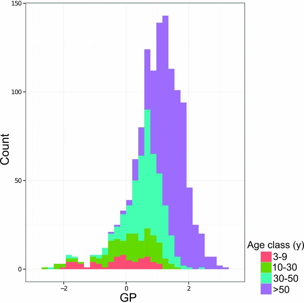
Figure 7. Histogram of gap phase (GP) values for the Wanang forest dynamics plot, Papua New Guinea, coloured by age class to show correspondence between gap phase and estimated time since disturbance.
Indicator species analysis of age classes in the Wanang FDP identified a total of 73 statistically significant indicator species, at least nine for each age class (Appendix 1). Many indicator species identified from the Wanang FDP appear in the DCA of chronosequence data (Appendix 2) labelled by priority of abundance (Appendix 3). In addition, there is correspondence between indicator species in the plot and our knowledge of life history variation (i.e. early versus late successional) in Wanang forest species.
DISCUSSION
Topography and soil nutrients
The variance partitioning analysis of basal area measurements suggested that forest structure was not explained by fine topographic or edaphic variation in the lowland rain forest of New Guinea, supporting our first hypothesis. Clark & Clark (Reference CLARK and CLARK2000) found little influence of topography and soil type on biomass distributions in 600 ha of rain forest in La Selva, Costa Rica. Conversely, at a landscape scale (plots spanning 1000 km), Laurance et al. (Reference LAURANCE, FEARNSIDE, LAURANCE, DELAMONICA, LOVEJOY, RANKIN-DE MERONA, CHAMBERS and GASCON1999) found that soil nutrients and soil water capacity parameters explained up to one third of variation in forest biomass in Amazonian terra firme forest. Both these studies used allometric equations to estimate biomass so the results from the Wanang forest in Papua New Guinea are not directly comparable since we based our analyses on basal area. However, basal area and biomass are related and comparisons of the general patterns found in all three studies are informative. A recent study from the Osa Peninsula, Costa Rica (Balzotti et al. Reference BALZOTTI, ASNER, TAYLOR, COLE, OSBORNE, CLEVELAND, PORDER and TOWNSEND2017), found that the density of large-basal-area, emergent canopy trees was influenced by topography. Spatial scale and soil characteristics are clearly important considerations when assessing landscape patterns of tree biomass and influence the consistency of results (Unger et al. Reference UNGER, HOMEIER and LEUSCHNER2012). Our study offers a fine-scale assessment of the relationship between overall basal area (as a proxy for biomass) and soil nutrients and suggests soils have little or no effect on basal area, at least at the 20 × 20-m scale, in the lowlands of New Guinea. This is likely caused by the apparent uniformly high soil fertility and dynamic landscape in New Guinea compared with the Osa Peninsula and Amazon basin. Our study incorporates basal area of all trees ≥1 cm but finer-scale topographical information (Chang et al. Reference CHANG, ZELENÝ, LI, CHIU and HSIEH2013) could influence the results.
Beyond overall basal area, soil nutrients and topography appear to account for smaller amounts of variation (0.29) in tree community composition in the study area in northern New Guinea compared with other tropical regions. For example, total variation explained ranged from 0.32 to 0.74 in a series of plots in the CTFS-ForestGEO network, including forests in South-East Asia, Africa and the neotropics (Baldeck et al. Reference BALDECK, HARMS, YAVITT, JOHN, TURNER, VALENCIA, NAVARRETE, DAVIES, CHUYONG, KENFACK, THOMAS, MADAWALA, GUNATILLEKE, GUNATILLEKE, BUNYAVEJCHEWIN, KIRATIPRAYOON, YAACOB, SUPARDI and DALLING2013). However, although the proportion of total variation accounted for by environmental variables was relatively small in the Wanang forest, providing partial support for our second hypothesis, it is apparent from the RGB map of local variation in community composition (Figure 3a) that some variation in composition in the Wanang tree community corresponds to major topographical features (Figure 1) such as ridges and gullies.
Environmental differences make it challenging to compare landscape variation in species composition across sites (Økland Reference ØKLAND1999) and sampling scale can greatly influence the detection of ecological patterns in diversity gradients (Tuomisto et al. Reference TUOMISTO, RUOKOLAINEN, VORMISTO, DUQUE, SÁNCHEZ, PAREDES and LÄHTEENOJA2017). Biotic interactions such as seed dispersal, insect herbivores and neighbourhood interactions also likely play a significant role in shaping species composition in this New Guinea forest as they do in all tropical forests (Leibold et al. Reference LEIBOLD, CHASE and ERNEST2017, Maron & Crone Reference MARON and CRONE2006, Uriarte et al. Reference URIARTE, CONDIT, CANHAM and HUBBELL2004). Another possibility is that we do not have sufficient resolution in our environmental data to detect trends associated with micro-topography and small-scale variation in soil nutrients. For example, our soil data in some cases showed extreme variation at scales smaller than 20 × 20 m, possibly caused by past landslips (Loffler Reference LOFFLER1977) that expose parent material and decouple the weathering and development of adjacent soils.
The instability of soils in New Guinea lowland rain forests may contribute to the relatively low overall basal area (Vincent et al. Reference VINCENT, HENNING, SAULEI, SOSANIKA and WEIBLEN2015), young age and high annual mortality rate. In fact, above-ground living biomass in the Wanang 50-ha plot, estimated at 211 Mg ha−1, is lower than the global mean estimate for lowland tropical forests (373 Mg ha−1) as well as the regional averages for Neotropical forests (288 Mg ha−1), Palaeotropical forests (393 Mg ha−1), Australian forests (514 Mg ha−1) and African forests (393 Mg ha−1) (Vincent et al. Reference VINCENT, HENNING, SAULEI, SOSANIKA and WEIBLEN2015).
Johns (Reference JOHNS1986) provided a qualitative description of the dynamic nature of New Guinea according to the frequency of major disturbances. These likely include high rainfall, unstable geology resulting from poorly consolidated marine sedimentary rock, and regular seismic activity from frequent strong earthquakes along the New Britain Trench. Garwood et al. (Reference GARWOOD, JANOS and BROKAW1979) contrasted the amount of land disturbed by earthquake-induced landslides in New Guinea and Panama, suggesting that 8–16% of land surface in New Guinea is disturbed per century compared with only 2% in Panama. Furthermore, erosional landslides in New Guinea disturb land at a rate of 3% per century, an order of magnitude greater than average rates measured in other landslide-prone areas such as the Luquillo mountains of Puerto Rico, which do suffer frequent hurricane impacts (Garwood et al. Reference GARWOOD, JANOS and BROKAW1979). The high frequency of earthquake-induced landslides illustrates the geological instability of the young, uplifted ocean sediments that make up much of the island of New Guinea. High rates of erosional surface wash can compound the likelihood of landslides that occur where a critical mass and height of forest trees has been achieved (Loffler Reference LOFFLER1977, Ruxton Reference RUXTON, Jennings and Mabbutt1967). The instability of the northern New Guinea landscape exposes fresh bedrock and leads to pedogenically young, fertile soils. Our analyses suggest increased disturbance resulting from landscape-level instability outweigh potentially positive effects of soil fertility on overall biomass accumulation.
Age class structure compared with chronosequence data
Previous dating of forest regeneration in the tropics has been confined to large-scale remote-sensing efforts (Kellner et al. Reference KELLNER, CLARK and HUBBELL2009) and methods relying on specific natural history, such as dating treefall gaps by palm morphology and growth rate (Martinez-Ramos et al. Reference MARTINEZ-RAMOS, ALVAREZ-BUYLLA, SARUKHAN and PINERO1988). Determining stand age in mixed broad-leaved forests with remote sensing (e.g. Landsat NDVI) is problematic (Foody et al. Reference FOODY, BOYD and CUTLER2003, Sader et al. Reference SADER, WAIDE, LAWRENCE and JOYCE1989), particularly in delineating younger successional stages (Nelson et al. Reference NELSON, KIMES, SALAS and ROUTHIER2000). We followed a different approach by corroborating comparisons of basal area in a reference chronosequence with indicator species analysis at a 20 × 20-m scale. In this way, we found evidence to support our third hypothesis of significant and frequent natural disturbance impacting basal area distributions and age-class structure in the New Guinea lowlands. Indicator species analyses rely on the assumption that changes to species composition through succession are similar across a given area. This assumption may not necessarily be true (Turner et al. Reference TURNER, WONG, CHEW and IBRAHIM1997) so rather than comparing overall composition, we relied on common indicator species to test correspondence in time since disturbance between mature forest and the chronosequence plots in nearby contiguous rain forest. We suggest that this use of chronosequences may provide an effective addition to remote sensing, particularly in the resolution of early successional stages. Interestingly, a previous study focused on forest regeneration following landslides, Guariguata (Reference GUARIGUATA1990) observed that basal area and floristic composition in Puerto Rican forests 50 y after landslides resembled that of pre-disturbance forest, a similar length of time to our observations in New Guinea.
Gap-phase dynamics
To further investigate patterns of tree size throughout the Wanang FDP, we used the gap-phase index (Feeley et al. Reference FEELEY, DAVIES, ASHTON, BUNYAVEJCHEWIN, NUR SUPARDI, KASSIM, TAN and CHAVE2007), to compare characteristics of New Guinea's lowland forest to other tropical regions. Generally, patterns were similar to those found in Panama, Cameroon and Malaysia (Feeley et al. Reference FEELEY, DAVIES, ASHTON, BUNYAVEJCHEWIN, NUR SUPARDI, KASSIM, TAN and CHAVE2007). However, extremes in gap phase differ between the BCI and Wanang FDPs. The BCI gap phase distribution is skewed towards higher GP values (mature forest plots dominated by large stems) whereas the Wanang FDP included some extremely low GP values (young secondary plots dominated by small stems). This contrast reflects an ecologically meaningful difference in the ratio of basal area in small and large stems in portions of the Wanang and BCI forests and provides support for our fourth hypothesis. It is worth noting that as calculated here, GP depends on total basal area at the 20 × 20-m scale in addition to the relative balance between small and large stems. Thus, observed patterns of GP may be affected by absolute basal area in each quadrat. However, previous comparisons (Vincent et al. Reference VINCENT, HENNING, SAULEI, SOSANIKA and WEIBLEN2015) suggest a substantial difference in the percentage of total biomass represented by small trees in the Wanang and BCI forests (7.21% versus 2.74% respectively).
Our plot dating results provide further support for the fourth hypothesis and corroborate the GP analysis, although these measures likely reveal different features of disturbance and forest recovery. The plot dating method we used is based on total basal area and is insensitive to remnant large trees in partly disturbed ‘young’ quadrats. By contrast, the GP index is a stem class ratio, which detects the presence of a large remnant tree, even if all other remaining stems are small. These two measures are complementary, but may vary with spatial scale and differ in indicating successional stage of regenerating forest. It is worth noting that our plot dating analysis suggested 18% of the Wanang FDP was either young or middle-aged secondary forest, disturbed in the past 30 y. This figure may be a conservative estimate since forest age in the Wanang FDP was based on comparisons with nearby areas of abandoned swidden agriculture. Naturally disturbed areas of mature rain forest might recover more rapidly through resprouting, the seed bank, and opportunistic growth by remnant trees (Guariguata & Ostertag Reference GUARIGUATA and OSTERTAG2001, Lawton & Putz Reference LAWTON and PUTZ1988, Nepstad et al. Reference NEPSTAD, UHL, PEREIRA and SILVA1996). On the other hand, other studies suggest that although species composition may proceed on different trajectories following agricultural disturbance (versus natural regeneration), basal area and stem density are comparable (Boucher et al. Reference BOUCHER, VANDERMEER, GRANZOW DE LA CERDA, MALLONA, PERFECTO and ZAMORA2001). Either way, the relatively large area of young forest and presence of extremely low GP values in the New Guinea forest suggest a dynamic community with relatively high rates of natural disturbance.
Comparison with other tropical forests
It appears that frequent landslides (Figure 8) and rapid surface erosion drive the difference in mortality rate between the Wanang FDP and lowland rain forests in Panama and Malaysia, the two best-studied forests in the CTFS-ForestGEO network. The high mortality reported for the subtropical Dingushan plot might also be attributed to erosion caused by extreme topography (260 m of altitudinal change in 20 ha) and also drought (the Dingushan forest is strongly seasonal) (Li et al. Reference LI, HUANG, YE, CAO, WEI, WANG, LIAN, SUN, MA and HE2009). Furthermore, it is worth noting that the Wanang FDP experiences higher mortality than other forests on similarly rugged topography with comparable annual rainfall. For example, annual tree mortality in the Palanan FDP in the north-eastern Philippines was 2.05%, increasing to 2.27% following the Category-four Typhoon Imbudo in 2003 (Yap et al. Reference YAP, DAVIES and CONDIT2016). The Lambir Hills FDP in Sarawak, Malaysian Borneo, experienced annual mortality rates of 1.3%, 1.75% and 1.66% before, during and following the 1997/1998 El Niño induced drought (Itoh et al. Reference ITOH, NANAMI, HARATA, OHKUBO, TAN, CHONG, DAVIES and YAMAKURA2012). This plot also has higher mean basal area than the Wanang FDP (42.8 m2 ha−1 versus 32.0 m2 ha−1). Thus, even forests experiencing severe natural disturbances appear to suffer lower mortality than background rates recorded at Wanang.

Figure 8. Example of a hillside slump close to the Wanang forest dynamics plot, Papua New Guinea. For scale, see one of the authors (GW) in a yellow tee-shirt in the upper centre portion of the image (Photo: TW).
A complete re-census of the Wanang FDP will allow us to investigate species- and size-class-specific mortality rates (Condit et al. Reference CONDIT, ASHTON, BUNYAVEJCHEWIN, DATTARAJA, DAVIES, ESUFALI, EWANGO, FOSTER, GUNATILLEKE, GUNATILLEKE, HALL, HARMS, HART, HERNANDEZ, HUBBELL, ITOH, KIRATIPRAYOON, LAFRANKIE, DE LAO and MAKANA2006) that are known to vary greatly (Coomes & Allen Reference COOMES and ALLEN2007). Of particular interest is the mortality rate of large trees (≥10 cm diameter at breast height), which we were unable to document as a separate size class in this study due to limited sample size. Previous studies in the BCI FDP and in Pasoh, Malaysia (King et al. Reference KING, DAVIES and NOOR2006, Condit et al. Reference CONDIT, PÉREZ, LAO, AGUILAR and HUBBELL2017), have documented high mortality rates in large trees during drought. Our slightly shorter census interval may have inflated the estimate of annual mortality since community-level mortality rate might change as a result of differences in intrinsic mortality rates of individual species (Lewis et al. Reference LEWIS, PHILLIPS, SHEIL, VINCETI, BAKER, BROWN, GRAHAM, HIGUCHI, HILBERT, LAURANCE, LEJOLY, MALHI, MONTEAGUDO, VARGAS, SONKE, SUPARDI, TERBORGH and MARTINEZ2004). In other words, as short-lived species die, the censused tree population is increasingly dominated by species with low mortality rates. However, since the mortality rate of trees in New Guinea is influenced by catastrophic events such as landslides that affect all species and size classes equally, we speculate that inflation of mortality rate would be low. In fact, a longer census interval would incorporate the effects of more landslides in addition to mortality events correlated with tree size and species identity.
In addition to natural disturbance, past human activity in the area might contribute to present day patterns. Small-scale shifting subsistence agriculture has been practiced in the Wanang forest for generations. However, aerial photographs from the early 1970s do not indicate gardens in the FDP for at least 50 y, although the effects of disturbance in the distant past might persist, as observed in the Amazon Basin (Levis et al. Reference LEVIS, COSTA, BONGERS, PEÑA-CLAROS, CLEMENT, JUNQUEIRA, NEVES, TAMANAHA, FIGUEIREDO, SALOMÃO, CASTILHO, MAGNUSSON, PHILLIPS, GUEVARA, SABATIER, MOLINO, LÓPEZ, MENDOZA, PITMAN and DUQUE2017).
CONCLUSION
We present the first detailed measurement of forest dynamics in New Guinea's lowland rain forests. The results support the reputation of New Guinea forests as dynamic in comparison to other lowland tropical forests. This characteristic of the New Guinea forest should be a consideration for global models of carbon storage and dynamics. As we hypothesized, basal area and age-class distribution in this New Guinea forest showed little or no relationship to variation in soil nutrients or topography, which appears to reflect frequent natural disturbances. In addition, mortality rates were generally higher and the forest was, overall, younger compared with other tropical forests. However, despite the dynamic nature we describe, species composition in New Guinea rain forests does reflect topography and soil fertility to a limited extent. Our results broaden understanding of the tropical forest biome and help place the dynamic New Guinea forests, which exist in an area of high tectonic activity, into a global context.
ACKNOWLEDGEMENTS
This work was supported by The Center for Tropical Forest Science and Forest Global Earth Observatories, the University of Minnesota Graduate School, Plant and Microbial Biology Graduate Program, and Bell Museum of Natural History. Census of the Wanang FDP was supported by the National Science Foundation (DEB-0816749), John Swire & Sons (PNG) Ltd and Steamships Trading Company, the Czech Science Foundation (16-18022S), and the UK Darwin Initiative for the Survival of Species. We thank the Wanang community for access to their forest and ongoing support. Members of the community who assisted with fieldwork include Matthew Kumba, Filip Damen, Albert Mansa and Dominic Rinan. We thank Dayana Agudo, Alexandra Bielnicka and Irene Torres for laboratory support. Staff at the New Guinea Binatang Center, including Chris Dahl, Pagi Toko, Bruce Isua, Martin Mogia, Maling Rimandai, Kenneth Molem, Joachim Yalang, Mavis Jimbudo, Nancy Labun, Gibson Sosanika and Billy Bau provided logistical support and field assistance. We also thank two anonymous reviewers whose comments and suggestions substantially improved the manuscript.
Appendix 1. Top 10 indicator species for each age class in the Wanang forest dynamics plot, Papua New Guinea. Statistically significant indicator species (P < 0.05) as determined by permutation are ranked by their indicator value statistic, indicating characteristic species that are abundant in a certain age class and present in most sites in that age class. The statistic being calculated following Dufrêne & Legendre (Reference DUFRÊNE and LEGENDRE1997) ranges from 0 to 1, with values closer to 1 indicating species that have higher fidelity and abundance in their associated habitat class. A full list of significant indicator species per age class is included in Appendix 3.
Appendix 2. Detrended correspondence analysis of tree species in nineteen 0.25-ha chronosequence plots located close to the Wanang forest dynamics plot, Papua New Guinea. Both plots (red) and species (black) are included. Proximity of plots to one another indicates similarity in species composition. Proximity of species to plot labels indicates fidelity to that particular forest type. Plot ages are denoted by the first letter of the corresponding label (M = mature, L = late secondary, E = early successional). Species names are plotted such that labels do not overlap, in the case of overlapping species name labels, preference was given to more abundant species.
Appendix 3. Table of all significant indicator species per age class in the Wanang forest dynamics plot, Papua New Guinea. Indicator value statistics and P-values are provided for each species identified as an indicator of an age class (*P ≤ 0.05, **P ≤ 0.01, ***P ≤ 0.001).