

1. Introduction
Climate change is the standard example of a negative externality, which should be addressed by an appropriate Pigovian tax. However, as argued by Carney (Reference Carney2015), climate change is a “tragedy of the horizon,” because its impact lies well beyond the horizon of most actors. While the political costs of enacting environmental regulation and raising eco-friendly taxes must be faced in the short term, the associated welfare and political gains are likely to emerge only in the medium to long term, suggesting that political-economy arguments may play an important role.Footnote 1
If governments are not in a comfortable position to raise taxes to tackle climate change, independent institutions such as central banks may be better placed to face the challenge: in January 2021, the Sverige Riksbank started a norm-based negative screening on purchases of corporate bonds; in July of the same year, the ECB announced a plan to entail climate considerations into its monetary policy framework including the transparency on emissions as an eligibility requirement and a possible tilting of its asset purchases program toward less carbon-intensive firms; in November, the Bank of England presented a plan with both negative screening and tilting towards less carbon-intensive firms among sectors.
According to several economists, a “Green Quantitative Easing” (Green QE) is an option on the table. Brunnermeier and Landau (Reference Brunnermeier and Landau2020) include Green QE among the tools available for central banks to address climate change and discuss whether independent institutions like central banks should pursue this route. Schoenmaker (Reference Schoenmaker2019) proposes to tilt the allocation of the Eurosystem’s assets and collateral towards low-carbon sectors, in order to reduce the cost of capital for these sectors relative to high-carbon sectors. De Grauwe (Reference De Grauwe2019) suggests that the ECB should replace the old bonds coming to maturity with new “environmental bonds,” which are issued to finance environmental projects. Other economists are rather skeptical about the feasibility of Green QE, given that it would break the principle of market neutrality. According to the then president of the Bundesbank Jens Weidmann, “Skewing asset purchases to green bonds, say, would run counter to this principle, which is anchored in Article 127 of the EU Treaty” [Weidmann (Reference Weidmann2019)].
In this paper, we merge the workhorse DSGE framework with an environmental model, in order to analyze the transmission mechanism of Green QE. We define Green QE as a central bank’s purchase of bonds issued by firms in non-polluting sectors, and we study its macroeconomic, environmental, and welfare effects through the lens of our model.
In the last decade, DSGE models have been commonly used to analyze the effects of QE.Footnote
2
DSGE models have been also used to study environmental policies. Heutel (Reference Heutel2012), Annicchiarico and Di Dio (Reference Annicchiarico and Di Dio2015), and Gibson and Heutel (Reference Gibson and Heutel2020) are applications of the benchmark environmental setup of Nordhaus (Reference Nordhaus2008), which includes an economic and a geophysical sector. In these models, production increases the flow of $\textrm{CO}_2$
emissions, which fuel the stock of atmospheric carbon (from now on we use the terms atmospheric carbon and pollution interchangeably). In turn, a higher atmospheric carbon reduces the total factor productivity of the economy: as highlighted by Nordhaus (Reference Nordhaus2008), pollutants such as
$\textrm{CO}_2$
emissions, which fuel the stock of atmospheric carbon (from now on we use the terms atmospheric carbon and pollution interchangeably). In turn, a higher atmospheric carbon reduces the total factor productivity of the economy: as highlighted by Nordhaus (Reference Nordhaus2008), pollutants such as $\textrm{CO}_2$
and other greenhouse gases are likely to affect the production possibilities of the world economy through their positive effects on global temperature.Footnote
3
Our model is the result of merging the DSGE framework of Gertler and Karadi (Reference Gertler and Karadi2011), designed to study QE, with the environmental model of Heutel (Reference Heutel2012), designed to study environmental policies over the business cycle. We calibrate the model to the euro area, where the ECB is planning to “adjust the framework guiding the allocation of corporate bond purchases to incorporate climate change criteria, in line with its mandate.”
$\textrm{CO}_2$
and other greenhouse gases are likely to affect the production possibilities of the world economy through their positive effects on global temperature.Footnote
3
Our model is the result of merging the DSGE framework of Gertler and Karadi (Reference Gertler and Karadi2011), designed to study QE, with the environmental model of Heutel (Reference Heutel2012), designed to study environmental policies over the business cycle. We calibrate the model to the euro area, where the ECB is planning to “adjust the framework guiding the allocation of corporate bond purchases to incorporate climate change criteria, in line with its mandate.”
In our model, we distinguish between two intermediate production sectors: the brown sector, whose production generates damaging emissions, and a green sector, whose production is not polluting. We interpret the two intermediate sectors as the providers of two sources of energy, whom a final-good firm uses to produce the good purchased by households and capital producers. This assumption allows to distinguish between bonds issued by green firms (green bonds) and bonds issued by brown firms (brown bonds). Bonds can be purchased by private banks and by the central bank. A leverage constraint prevents banks to fully exploit the arbitrage opportunity between bonds and deposits from households: in equilibrium, there is a spread between the bond and the deposit interest rate.
The paper crucially depends on two important assumptions, which we spell out upfront. First, we study the transmission mechanism of Green QE assuming that the government does not introduce any environmental policy, such as carbon taxes: even if this may seem an unrealistic assumption—after all the government is the main responsible for environmental policy—we prefer to isolate the transmission mechanism of Green QE. Second, we assume that monetary policy, both conventional and unconventional, is neutral in the long run, as is standard assumption in the DSGE literature; this means that a permanent Green QE has no impact in the long run. Therefore, we only study the transmission mechanism of a temporary Green QE and the short-term impact of a permanent Green QE.
We simulate two types of Green QE: a Green QE that does not change the size of central bank’s balance sheet; a Green QE that increases the size of central bank’s balance sheet. It is well known that QE can work only if Wallace neutrality does not hold. As Wallace (Reference Wallace1981) points out, the equilibrium path of output and prices is independent from central bank’s balance sheet policies, unless there is something special in central bank’s intermediation. In our model, QE does affect production, because the central bank, as opposed to private banks, does not face leverage constraints. If the central bank temporarily expands its balance sheet by increasing holding of green and brown bonds, banks reduce their leverage, the credit spread goes down, and output grows. This is the mechanism at the heart of Gertler and Karadi (Reference Gertler and Karadi2011). If green and brown bonds are perfect substitutes for banks, when the central bank temporarily tilts the portfolio composition to green bonds keeping the size of the balance sheet constant, production in both sectors is not affected. Without further assumptions, even in a model where QE works, this balance sheet neutral Green QE is not able to affect total production and damaging emissions. The intuition relies on a no-arbitrage condition. If green and brown bonds are perfect substitutes for banks, their returns must be identical as well. In this case, the portfolio rebalancing of the central bank determined by Green QE is fully offset by a rebalancing of private banks in the opposite direction. Under this scenario, Green QE only implies a transaction between private banks and the central bank, with neither macroeconomic nor environmental effect. As a result of the same intuition, a Green QE that increases the size of central bank’s balance sheet has the same effects of a market-neutral QE.
In order to explore the role of Green QE, we make green and brown bonds imperfect substitutes.Footnote 4 We do so by introducing a quadratic cost whenever a bank changes the composition of its portfolio with respect to the steady-state level.Footnote 5 Under this hypothesis, the share of bank’s green bonds out of bank’s total assets is a positive function of the spread between green and brown bonds: the higher the interest rate paid by green bonds relatively to brown bonds, the more banks invest in the green sector.
Having a model suited to study Green QE, we perform several exercises.
First, we simulate a temporary Green QE shock. When the central bank temporarily increases its share of green bonds, keeping constant total assets, the interest rate paid by green (brown) firms decrease (increase). Banks are not able to fully exploit the arbitrage opportunity, because changing the asset composition is costly: a spread between brown and green interest rates opens up. Green firms face a lower interest rate, increase capital, and raise production. Brown firms face a higher interest rate and cut production: detrimental emissions are lower and decrease the stock of atmospheric carbon. The production externality is reduced and total factor productivity increases. From a quantitative perspective, the reduction in emissions is tiny. The fall in global pollution (the relevant variable for the TFP externality) is negligible, also because euro-area emissions contribute only by about $6.5\%$
to global emissions; moreover, the stock of pollution is two orders of magnitude larger than the quarterly flow of global emissions.
$6.5\%$
to global emissions; moreover, the stock of pollution is two orders of magnitude larger than the quarterly flow of global emissions.
Second, we simulate a temporary increase in central bank’s total assets comparing two different scenarios. In the first scenario, we assume that central bank’s purchases are market neutral. In the second scenario, we assume that QE is entirely targeted to green bonds. We show that the effect on emissions is very small also in this case.
Third, we design a Taylor rule for Green QE, assuming that the fraction of central bank’s green assets endogenously respond to emissions. We simulate a positive TFP shock, comparing the response of the economy with and without the Green QE rule. We find that the policy is able to slightly contain the rise in emissions. We compute numerically the parameter of the Green QE rule that maximizes welfare after a positive TFP shock. This parameter governs the elasticity of Green QE to emissions. We find that the central bank should respond to emissions only if there are no intermediation costs, that is when the central bank is as effective as the private sector in intermediate funds; even in this case, the net welfare gains of Green QE are extremely small.
Fourth, we modify our baseline model to study a permanent Green QE that sells the entire stock of brown bonds held by the central bank forever. We highlight which assumptions are necessary to make a permanent Green QE effective at least in the short run. We show that the effects of Green QE are much more persistent on the flow of emissions, but still tiny.
We aim at contributing to the scant yet rapidly growing DSGE literature on how central banks’ instruments can address environmental issues or the consequences of the green transition. In particular, Carattini et al. (Reference Carattini, Heutel and Melkadze2021) use a framework similar to our model to study whether environmental policy may lead to financial-macroeconomic risk; in a paper complementary to our work, Giovanardi et al. (Reference Giovanardi, Kaldorf, Radke and Wicknig2021) analyze the effects of reducing the haircut applied by the central bank to green bonds that are used as collateral in refinancing operations, a proposal widely discussed in policy and academic circles; Ferrari Minesso and Pagliari (Reference Ferrari Minesso and Pagliari2021) and Bartocci et al. (Reference Bartocci, Notarpietro and Pisani2022) analyze the interactions of monetary and green fiscal policies in a two-country environmental DSGE model; in a follow-up paper, we study a permanent Green QE, along the transition to a zero-emission economy [Ferrari and Nispi Landi (Reference Ferrari and Nispi Landi2022)], an exercise carried out also by Abiry et al. (Reference Abiry, Ferdinandusse, Ludwig and Nerlich2022).
The papers closest to our work are Dafermos et al. (Reference Dafermos, Nikolaidi and Galanis2018), Diluiso et al. (Reference Diluiso, Annicchiarico, Kalkuhl and Minx2021), and Benmir and Roman (Reference Benmir and Roman2020). Using a stock-flow-fund model, Dafermos et al. (Reference Dafermos, Nikolaidi and Galanis2018) assess the financial and global warming implications of Green QE. Unlike Dafermos et al. (Reference Dafermos, Nikolaidi and Galanis2018), we use a microfunded DSGE model to study Green QE. In a contemporaneous work, Diluiso et al. (Reference Diluiso, Annicchiarico, Kalkuhl and Minx2021) develop a DSGE model to study the financial stability implications of climate change and of the transition toward a green economy. Benmir and Roman (Reference Benmir and Roman2020) study the optimal macroecononic-environmental policy mix in a DSGE model. In one experiment, both Diluiso et al. (Reference Diluiso, Annicchiarico, Kalkuhl and Minx2021) and Benmir and Roman (Reference Benmir and Roman2020) study a Green QE policy. Unlike these two papers, we exclusively focus on Green QE, and we crucially assume that banks cannot fully arbitrage green and brown bonds: this assumption is fundamental for Green QE to affect the spread between green and brown interest rates.
The rest of the paper is organized as follows. Section 2 presents the model. In Section 3, we analyze the transmission channel of different versions of a temporary Green QE. In Section 4, we study a permanent Green QE. In Section 5, we perform a sensitivity analysis. Section 6 concludes.
2. Model
We merge the financial accelerator framework of Gertler and Karadi (Reference Gertler and Karadi2011) with the environmental model of Heutel (Reference Heutel2012), which in turn is a simplified version of Nordhaus (Reference Nordhaus2008). Our model features two production sectors: a brown sector, which generates a pollution externality affecting total factor productivity, and a green sector, which does not pollute. Two different sectors are crucial to distinguish between green bonds and brown bonds. Green and brown firms sell their goods to a continuum of intermediate firms. These firms operate in monopolistic competition and are subject to price adjustment costs. A final-good firm combines the differentiated intermediate goods to produce a final good. The final good is bought by households for consumption and by capital producers, which transform it in physical capital. Households can be either workers in green and brown firms or bankers. Bankers collect deposits from households and buy bonds issued by green and brown firms. In what follows, we lay out the optimization problems of all the agents of the model. We leave the full list of equations to Online Appendix B.
2.1. Households
There is a continuum of households of measure unity. In any period, a fraction $1-f$
of households are workers, a fraction
$1-f$
of households are workers, a fraction $f$
are bankers. Every banker stays banker in the next period with probability
$f$
are bankers. Every banker stays banker in the next period with probability $\chi$
: in every period
$\chi$
: in every period $ (1-\chi )f$
, bankers become worker. We assume that
$ (1-\chi )f$
, bankers become worker. We assume that $ (1-\chi )f$
workers randomly become bankers and the proportion remains unchanged. Each banker manages a bank and transfers profits to households. Different households completely share idiosyncratic risk: this assumption allows to use the representative household framework.
$ (1-\chi )f$
workers randomly become bankers and the proportion remains unchanged. Each banker manages a bank and transfers profits to households. Different households completely share idiosyncratic risk: this assumption allows to use the representative household framework.
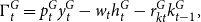
The representative household solves the following optimization problem:
 \begin{align*} \max _{\left \{ c_{t},h_{t},d_{Ht}\right \} _{t=0}^{\infty }}\mathbb{E}_{0}\sum _{t=0}^{\infty }\beta ^{t}\!\left (\frac{c_{t}^{1-\sigma }}{1-\sigma }-\frac{h_{t}^{1+\varphi }}{1+\varphi }\right )\\[5pt] s.t.\ c_{t}+d_{Ht}=\frac{r_{t-1}}{\pi _{t}}d_{Ht-1}+w_{t}h_{t}-t_{t}+\Gamma _{t}, \end{align*}
where $c_t$
denotes consumption of the final good;
$c_t$
denotes consumption of the final good; $h_t$
denotes hours worked;
$h_t$
denotes hours worked; $d_{Ht}$
is the sum of bank deposits
$d_{Ht}$
is the sum of bank deposits $d_t$
; and monetary base
$d_t$
; and monetary base $b_{Pt}$
: both assets are expressed in real terms and yield a nominal interest rate
$b_{Pt}$
: both assets are expressed in real terms and yield a nominal interest rate $r_t$
;Footnote
6
$r_t$
;Footnote
6 $w_t$
is hourly real wage;
$w_t$
is hourly real wage; $\pi _t$
is CPI gross inflation rate;
$\pi _t$
is CPI gross inflation rate; $t_t$
denote lump-sum taxes;
$t_t$
denote lump-sum taxes; $\Gamma _t$
are profits from ownership of firms and net transfers from banks. First-order conditions read:
$\Gamma _t$
are profits from ownership of firms and net transfers from banks. First-order conditions read:
 \begin{align} h_{t}^{\varphi }c_t^\sigma = w_{t} \end{align}
 \begin{align} c_t^{-\sigma } = \beta \mathbb{E}_{t}\!\left (c_{t+1}^{-\sigma }\frac{r_{t}}{\pi _{t+1}}\right ). \end{align}
2.2. Final-good firms
The representative final-good firm uses the following CES aggregator to produce the final good $y_{t}$
:
$y_{t}$
:
 \begin{equation} y_{t}=\left [\int _{0}^{1}y_{t}(i)^{\frac{\varepsilon -1}{\varepsilon }}di\right ]^{\frac{\varepsilon }{\varepsilon -1}}, \end{equation}
where $y_{t} (i )$
is an intermediate good produced by intermediate firm
$y_{t} (i )$
is an intermediate good produced by intermediate firm $i$
, whose price is
$i$
, whose price is $p_{t} (i )$
. The problem of the final-good firm is the following:
$p_{t} (i )$
. The problem of the final-good firm is the following:
 \begin{align*} \max _{y_{t},\left \{ y_{t}\left (i\right )\right \} _{i\in \left [0,1\right ]}}p_{t}y_{t}-\int _{0}^{1}p_{t}(i)y_{t}(i)di\\[5pt] s.t\ y_{t}=\left [\int _{0}^{1}y_{t}(i)^{\frac{\varepsilon -1}{\varepsilon }}di\right ]^{\frac{\varepsilon }{\varepsilon -1}}, \end{align*}
where $p_t$
is the CPI. This problem yields the following demand function
$p_t$
is the CPI. This problem yields the following demand function $\forall i$
:
$\forall i$
:
 \begin{equation} y_{t}(i)=y_{t}\!\left (\frac{p_{t}(i)}{p_{t}}\right )^{-\varepsilon }. \end{equation}
2.3. Intermediate-good firms
There is a continuum of firms indexed by $i$
, producing a differentiated input and using the following function:
$i$
, producing a differentiated input and using the following function:
 \begin{equation} y_{t}\!\left (i\right )=y_{t}^{I}\!\left (i\right ), \end{equation}
where $y_{t}^{I}$
is a CES bundle of green production
$y_{t}^{I}$
is a CES bundle of green production $y_t^G$
and brown production
$y_t^G$
and brown production $y_t^B$
:
$y_t^B$
:
 \begin{equation} y_{t}^{I}\!\left (i\right )=\left [\left (1-\zeta \right )^{\frac{1}{\xi }}\!\left (y_{t}^{G}\!\left (i\right )\right )^{\frac{\xi -1}{\xi }}+\zeta ^{\frac{1}{\xi }}\!\left (y_{t}^{B}\!\left (i\right )\right ){}^{\frac{\xi -1}{\xi }}\right ]^{\frac{\xi }{\xi -1}}. \end{equation}
The intermediate firm $i$
solves an intratemporal problem to choose the optimal input combination and an intertemporal problem to set the price. The intratemporal problem, that is minimizing costs subject to a given level of production, reads:
$i$
solves an intratemporal problem to choose the optimal input combination and an intertemporal problem to set the price. The intratemporal problem, that is minimizing costs subject to a given level of production, reads:
 \begin{align*} & \min _{y_{t}^{B}\!\left (i\right ),y_{t}^{G}\!\left (i\right )} p_{t}^{G}y_{t}^{G}\!\left (i\right )+p_{t}^{B}y_{t}^{B}\!\left (i\right )\\[5pt] & s.t.\ \left [\left (1-\zeta \right )^{\frac{1}{\xi }}\!\left (y_{t}^{G}\!\left (i\right )\right )^{\frac{\xi -1}{\xi }}+\zeta ^{\frac{1}{\xi }}\!\left (y_{t}^{B}\!\left (i\right )\right ){}^{\frac{\xi -1}{\xi }}\right ]^{\frac{\xi }{\xi -1}}=y_{t}^I\!\left (i\right ), \end{align*}
where $p_{t}^{G}$
and
$p_{t}^{G}$
and $p_{t}^{B}$
are the prices of green and brown production, respectively, expressed relatively to the CPI;
$p_{t}^{B}$
are the prices of green and brown production, respectively, expressed relatively to the CPI; $y_t^I (i )$
is taken as given. The problem yields the following demand functions for the green and brown input:
$y_t^I (i )$
is taken as given. The problem yields the following demand functions for the green and brown input:
 \begin{align} y_{t}^{G}\!\left (i\right )&=\left (1-\zeta \right )\left (\frac{p_{t}^{G}}{p_{t}^{I}}\right )^{-\xi }y_{t}^{I}\!\left (i\right ) \end{align}
 \begin{align} y_{t}^{B}\!\left (i\right ) & =\zeta \!\left (\frac{p_{t}^{B}}{p_{t}^{I}}\right )^{-\xi }y_{t}^{I}\!\left (i\right ), \end{align}
where $p_{t}^{I}=\left [\left (1-\zeta \right )\left (p_{t}^{G}\right )^{1-\xi }+\zeta \!\left ( p_{t}^B\right )^{1-\xi }\right ]^{\frac{1}{1-\xi }}$
is the real marginal cost of the firm.
$p_{t}^{I}=\left [\left (1-\zeta \right )\left (p_{t}^{G}\right )^{1-\xi }+\zeta \!\left ( p_{t}^B\right )^{1-\xi }\right ]^{\frac{1}{1-\xi }}$
is the real marginal cost of the firm.
Firms operate in monopolistic competition, so they set prices subject to the demand of the final-good firm (4). Firm $i$
pays quadratic adjustment costs
$i$
pays quadratic adjustment costs $\textrm{AC}_{t} (i)$
in nominal terms, whenever it adjusts its price inflation with respect to the central bank’s target
$\textrm{AC}_{t} (i)$
in nominal terms, whenever it adjusts its price inflation with respect to the central bank’s target $\overline{\pi }$
:
$\overline{\pi }$
:
 \begin{equation*} \textrm{AC}_{t}\!\left (i\right )=\frac {\kappa _{P}}{2}\!\left (\frac {p_{t}\!\left (i\right )}{p_{t-1}\!\left (i\right )}-\overline {\pi }\right )^{2}p_{t}y_{t}. \end{equation*}
Firm $i$
’s intertemporal maximization problem reads:
$i$
’s intertemporal maximization problem reads:
 \begin{equation*} \max _{\left \{ p_{t}\!\left (i\right )\right \} _{t=0}^{\infty }}\mathbb {E}_{0}\!\left \{ \sum _{t=0}^{\infty }\beta ^{t}\frac {\lambda _{t}}{\lambda _{0}}\!\left [\left (\frac {p_{t}(i)}{p_{t}}\right )^{-\varepsilon }\!\left (\frac {p_{t}\!\left (i\right )}{p_{t}}-p_{t}^{I}\right )y_{t}-\frac {\kappa _{P}}{2}\!\left (\frac {p_{t}\!\left (i\right )}{p_{t-1}\!\left (i\right )}-\overline {\pi }\right )^{2}y_{t}\right ]\right \}, \end{equation*}
where $\lambda _t$
is the marginal utility of households. In a symmetric equilibrium, this problem yields a non-linear Phillips Curve:
$\lambda _t$
is the marginal utility of households. In a symmetric equilibrium, this problem yields a non-linear Phillips Curve:
 \begin{equation} \pi _{t}\!\left (\pi _{t}-\overline{\pi }\right ) =\beta \mathbb{E}_{t}\!\left [\frac{\lambda _{t+1}}{\lambda _{t}}\pi _{t+1}\left (\pi _{t+1}-\overline{\pi }\right )\frac{y_{t+1}}{y_{t}}\right ]+\frac{\varepsilon }{\kappa _{P}}\!\left (p_{t}^{I}-\frac{\varepsilon -1}{\varepsilon }\right ). \end{equation}
2.4. Green and brown firms
Green and brown firms produce an output good that is used as an input by intermediate firms. Green firms use the following function to produce $y_{t}^{G}$
:
$y_{t}^{G}$
:
 \begin{equation} y_{t}^{G}=A_{t}\!\left (k_{t-1}^{G}\right )^{\alpha }\!\left (h_{t}^G\right )^{1-\alpha }, \end{equation}
where $k_{t}^{G}$
and
$k_{t}^{G}$
and $h_t^G$
are capital and labor used in the green sector;
$h_t^G$
are capital and labor used in the green sector; $A_{t}$
is total factor productivity, which is endogenous: we explain in detail what drives total factor productivity in Section 2.7. Green firms issue bonds
$A_{t}$
is total factor productivity, which is endogenous: we explain in detail what drives total factor productivity in Section 2.7. Green firms issue bonds $b_{t}^{G}$
to finance capital expenditure:
$b_{t}^{G}$
to finance capital expenditure:
 \begin{equation} b_{t}^{G}=q_{t}k_{t}^{G}, \end{equation}
where $q_{t}$
is the price of the capital good. The bond is expressed in real terms and pay a real interest rate
$q_{t}$
is the price of the capital good. The bond is expressed in real terms and pay a real interest rate $r_{t}^{G}$
. Green firms buy capital from capital producers, which in turn buy back non-depreciated capital from green firms. In period
$r_{t}^{G}$
. Green firms buy capital from capital producers, which in turn buy back non-depreciated capital from green firms. In period $t$
, profits
$t$
, profits $\Gamma _{t}^{G}$
of green firms are given by:
$\Gamma _{t}^{G}$
of green firms are given by:
 \begin{equation} \Gamma _{t}^{G} = p_{t}^{G}y_{t}^{G}-w_{t}h_{t}^{G}-r_{kt}^{G}k_{t-1}^{G}, \end{equation}
where
 \begin{equation} r_{kt}^{G}\equiv r_{t}^{G}q_{t-1}-\left (1-\delta \right )q_{t} \end{equation}
is the rental rate of capital for green firms. First-order conditions for green firms read:
 \begin{align} w_{t}h_{t}^{G} & =\left (1-\alpha \right )p_{t}^{G}y_{t}^{G} \end{align}
 \begin{align} r_{kt}^{G}k_{t-1}^{G} & =\alpha p_{t}^{G}y_{t}^{G}. \end{align}
The brown sector is modeled analogously, and it comprises the following equations:
 \begin{align} y_{t}^{B}&=A_{t}\!\left (k_{t-1}^{B}\right )^{\alpha }\!\left (h_{t}^B\right )^{1-\alpha } \end{align}
 \begin{align} w_{t}h_{t}^{B} & =\left (1-\alpha \right )p_{t}^{B}y_{t}^{B} \end{align}
 \begin{align} r_{kt}^{B}k_{t-1}^{B} & =\alpha p_{t}^{B}y_{t}^{B} \end{align}
 \begin{align} b_{t}^{B} & =q_{t}k_{t}^{B} \end{align}
 \begin{align} r_{kt}^{B} & =r_{t}^{B}q_{t-1}-\left (1-\delta \right )q_{t}. \end{align}
2.5. Capital producers
Capital producers buy the output produced by final-good firms and non-depreciated capital from intermediate firms, in order to produce physical capital. Capital is then purchased by green and brown firms. Capital producers solve the following problem:
 \begin{align*} \max _{\left \{ i_{t},k_{t}\right \} _{t=0}^{\infty }}\mathbb{E}_{0}\!\left \{ \sum _{t=0}^{\infty }\beta ^{t}\frac{\lambda _{t}}{\lambda _{0}}\!\left [q_{t}k_{t}-\left (1-\delta \right )q_{t}k_{t-1}-i_{t}\right ]\right \} \\[5pt] s.t.\ k_{t}=\left (1-\delta \right )k_{t-1}+\left [1-\frac{\kappa _{I}}{2}\!\left (\frac{i_{t}}{i_{t-1}}-1\right )^{2}\right ]i_{t}, \end{align*}
where $k_t$
is aggregate capital in the economy and
$k_t$
is aggregate capital in the economy and $i_t$
denotes investment. The first-order condition reads:
$i_t$
denotes investment. The first-order condition reads:
 \begin{eqnarray} q_{t}\!\left \{ 1-\frac{\kappa _{I}}{2}\!\left (\frac{i_{t}}{i_{t-1}}-1\right )^{2}-\kappa _{I}\frac{i_{t}}{i_{t-1}}\!\left (\frac{i_{t}}{i_{t-1}}-1\right )\right \} +\beta \mathbb{E}_{t}\!\left [\frac{\lambda _{t+1}}{\lambda _{t}}q_{t+1}\!\left (\frac{i_{t+1}}{i_{t}}\right )^{2}\kappa _{I}\!\left (\frac{i_{t+1}}{i_{t}}-1\right )\right ] & = & 1.\nonumber \\[5pt] \end{eqnarray}
2.6. Banks
We first present a version of the banking sector with no financial frictions, in order to illustrate which assumptions are necessary for QE and Green QE to work. Second, we describe the model used in the simulations, where the banking sector does face financial frictions.
2.6.1. No financial frictions
There is a continuum of banks indexed by $j$
. The balance sheet of bank
$j$
. The balance sheet of bank $j$
is given by:
$j$
is given by:
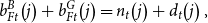 \begin{equation} b_{Ft}^{B}\!\left (j\right )+b_{Ft}^{G}\!\left (j\right )=n_{t}\!\left (j\right )+d_{t}\!\left (j\right ), \end{equation}
where $b_{Ft}^{B} (j )$
and
$b_{Ft}^{B} (j )$
and $b_{Ft}^{G} (j )$
are green and brown bonds purchased by bank
$b_{Ft}^{G} (j )$
are green and brown bonds purchased by bank $j$
;
$j$
; $n_{t} (j )$
is bank
$n_{t} (j )$
is bank $j$
’s net worth, which accumulates through profits:
$j$
’s net worth, which accumulates through profits:
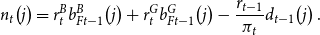 \begin{equation} n_{t}\!\left (j\right ) =r_{t}^{B}b_{Ft-1}^{B}\!\left (j\right )+r_{t}^{G}b_{Ft-1}^{G}\!\left (j\right )-\frac{r_{t-1}}{\pi _{t}}d_{t-1}\!\left (j\right ). \end{equation}
Let $\beta ^{i}\Lambda _{t,t+i}$
be the stochastic discount factor applying in
$\beta ^{i}\Lambda _{t,t+i}$
be the stochastic discount factor applying in $t$
to earnings in
$t$
to earnings in $t+i$
, where
$t+i$
, where $\Lambda _{t,t+i}\equiv \frac{\lambda _{t+i}}{\lambda _{t}}$
. With probability
$\Lambda _{t,t+i}\equiv \frac{\lambda _{t+i}}{\lambda _{t}}$
. With probability $ (1-\chi )$
, banker
$ (1-\chi )$
, banker $j$
exits the market getting
$j$
exits the market getting $n_{t+1} (j )$
at the beginning of period
$n_{t+1} (j )$
at the beginning of period $t+1$
: these resources are transferred to households. With probability
$t+1$
: these resources are transferred to households. With probability $\chi$
, banker
$\chi$
, banker $j$
continues the activity, getting the continuation value. The value of bank
$j$
continues the activity, getting the continuation value. The value of bank $j$
is defined as follows:
$j$
is defined as follows:
 \begin{equation} V_{jt}\!\left (n_{t}\!\left (j\right )\right ) =\max \mathbb{E}_{t}\!\left [\sum _{i=0}^{\infty }\!\left (1-\chi \right )\chi ^{i}\beta ^{i+1}\Lambda _{t,t+1+i}n_{t+1+i}\!\left (j\right )\right ]. \end{equation}
Absent financial frictions, up to a first-order approximation the optimization problem implies the following interest parity conditions:
 \begin{equation} \tilde{rr}_t=\mathbb{E}_t \!\left (\tilde{r}_{t+1}^G\right )=\mathbb{E}_t \!\left (\tilde{r}_{t+1}^B\right ), \end{equation}
where variables with tilde denote percentage deviations from the steady state, and $rr_t\equiv \mathbb{E}_t \!\left (\frac{r_t}{\pi _{t+1}}\right )$
is the real interest rate. The first equality prevents QE to be effective. Any increase in real monetary base (which yields the real interest rate) to finance purchase of corporate bonds by the central bank is offset by a sale of corporate bonds by the banking sector, up to the point that the first equality of equation (25) always holds:Footnote
7
QE is not able to affect interest rates.
$rr_t\equiv \mathbb{E}_t \!\left (\frac{r_t}{\pi _{t+1}}\right )$
is the real interest rate. The first equality prevents QE to be effective. Any increase in real monetary base (which yields the real interest rate) to finance purchase of corporate bonds by the central bank is offset by a sale of corporate bonds by the banking sector, up to the point that the first equality of equation (25) always holds:Footnote
7
QE is not able to affect interest rates.
The second equality of equation (25) prevents Green QE to be effective. Any increase in green bonds held by the central bank financed with a sale of brown bonds is fully offset by an opposite transaction by the banking sector, up to the point that the second equality of equation (25) always holds: Green QE is not able to affect the green-brown spread, and so it is not able to shift production from the brown to the green sector.
Absent financial frictions, deposits and corporate bonds are perfect substitutes, so they yield the same return. Moreover, within corporate bonds, green and brown bonds are perfect substitutes too, and green and brown interest rates are equal.
2.6.2. Financial frictions
We introduce two financial frictions in the model, in order to break the two equalities of equation (25), making deposits, green, and corporate bonds imperfect substitutes.
First, following Gertler and Karadi (Reference Gertler and Karadi2011), we assume that in every period bankers can divert a fraction $\theta$
of available funds. If they do so, depositors can recover the remaining fraction of the assets. Depositors are willing to lend to bankers if and only if the value of the bank is not lower than the fraction of divertable funds:
$\theta$
of available funds. If they do so, depositors can recover the remaining fraction of the assets. Depositors are willing to lend to bankers if and only if the value of the bank is not lower than the fraction of divertable funds:
 \begin{equation} V_{jt}\!\left (n_{t}\!\left (j\right )\right )\geq \theta b_{Ft}\!\left (j\right ), \end{equation}
where $b_{Ft} (j ) \equiv b_{Ft}^{B} (j )+b_{Ft}^{G} (j )$
denotes total assets of bank
$b_{Ft} (j ) \equiv b_{Ft}^{B} (j )+b_{Ft}^{G} (j )$
denotes total assets of bank $j$
. Given that banks are constrained, they cannot fully arbitrage between assets and liabilities, and a spread between interest rates on corporate bonds and deposits emerges in equilibrium: the first equality in equation (25) does not hold anymore. By doing QE, the central bank is able to affect the spread and, as a consequence, to affect the real economy. However, this friction is neither necessary nor sufficient to make Green QE work, because it does not break the equality between green and brown rates. We still keep the friction because it makes sense for us studying Green QE in a framework typically used to analyze QE. More importantly, we can analyze the scenario in which the purchase of green bonds is financed with higher monetary base.Footnote
8
$j$
. Given that banks are constrained, they cannot fully arbitrage between assets and liabilities, and a spread between interest rates on corporate bonds and deposits emerges in equilibrium: the first equality in equation (25) does not hold anymore. By doing QE, the central bank is able to affect the spread and, as a consequence, to affect the real economy. However, this friction is neither necessary nor sufficient to make Green QE work, because it does not break the equality between green and brown rates. We still keep the friction because it makes sense for us studying Green QE in a framework typically used to analyze QE. More importantly, we can analyze the scenario in which the purchase of green bonds is financed with higher monetary base.Footnote
8
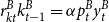
Second, in order to break the equality between green and brown rates, we assume that banks pay a quadratic cost when they change the fraction of green bonds out of total bonds with respect to the steady-state level $b^*$
. The law of motion of bank
$b^*$
. The law of motion of bank $ (j )$
’s net worth becomes:
$ (j )$
’s net worth becomes:
 \begin{align} n_{t}\!\left (j\right ) & =r_{t}^{B}b_{Ft-1}^{B}\!\left (j\right )+r_{t}^{G}b_{Ft-1}^{G}\!\left (j\right )-\frac{r_{t-1}}{\pi _{t}}d_{t-1}\!\left (j\right )-\frac{\kappa _{FG}}{2}n_{t-1}\!\left (j\right )\!\left (\frac{b_{Ft-1}^{G}\!\left (j\right )}{b_{Ft-1}\!\left (j\right )}-b^{*}\right )^{2}. \end{align}
This friction is one of the reduced-form assumptions that are widely used in the literature to make two different assets imperfect substitutes. The implication of these assumptions is a relative demand between two assets that is an increasing function of the interest rate spread between these assets: the higher the interest rate on asset $x$
relatively to the rate on asset
$x$
relatively to the rate on asset $y$
, the more investors buy
$y$
, the more investors buy $x$
and sell
$x$
and sell $y$
. These bond-demand functions date back at least to Tobin (Reference Tobin1969), which explicitly models asset demands as increasing functions of asset returns in an IS-LM model. In a DSGE model, Andres et al. (Reference Andres, López-Salido and Nelson2004) introduce a quadratic cost when households change the allocation between money and long-term bonds, with respect to the steady state: their goal is to derive a long-term bond demand that is increasing in the long-term interest rate, in the same spirit of Tobin. In order to study QE, Chen et al. (Reference Chen, Cúrdia and Ferrero2012) assume that long-term public bonds pay an endogenous risk premium, which is in an increasing function of the outstanding stock of long-term public bonds: they obtain a demand for long-term public bonds that is increasing in the spread between long- and short-term rates. On top of these contributions, a quadratic adjustment cost on foreign bonds is a standard assumption in open-economy models, in order to break the parity condition between domestic and foreign interest rates: this assumption is required to make an open-economy model stationary and with a determinate steady state,Footnote
9
and it is a useful friction to give a role to FX interventions [Alla et al. (Reference Alla, Espinoza and Ghosh2020)] and to capital controls [Nispi Landi (Reference Nispi Landi2020)]. The shortcoming of the quadratic cost assumption is the lack of deep microfoundations, which makes these models (and ours) vulnerable to the Lucas Critique: in order to alleviate this important concern, we show that our results are robust qualitatively to
$y$
. These bond-demand functions date back at least to Tobin (Reference Tobin1969), which explicitly models asset demands as increasing functions of asset returns in an IS-LM model. In a DSGE model, Andres et al. (Reference Andres, López-Salido and Nelson2004) introduce a quadratic cost when households change the allocation between money and long-term bonds, with respect to the steady state: their goal is to derive a long-term bond demand that is increasing in the long-term interest rate, in the same spirit of Tobin. In order to study QE, Chen et al. (Reference Chen, Cúrdia and Ferrero2012) assume that long-term public bonds pay an endogenous risk premium, which is in an increasing function of the outstanding stock of long-term public bonds: they obtain a demand for long-term public bonds that is increasing in the spread between long- and short-term rates. On top of these contributions, a quadratic adjustment cost on foreign bonds is a standard assumption in open-economy models, in order to break the parity condition between domestic and foreign interest rates: this assumption is required to make an open-economy model stationary and with a determinate steady state,Footnote
9
and it is a useful friction to give a role to FX interventions [Alla et al. (Reference Alla, Espinoza and Ghosh2020)] and to capital controls [Nispi Landi (Reference Nispi Landi2020)]. The shortcoming of the quadratic cost assumption is the lack of deep microfoundations, which makes these models (and ours) vulnerable to the Lucas Critique: in order to alleviate this important concern, we show that our results are robust qualitatively to $\kappa _{FG}$
, which captures the importance of the adjustment costs, and it is has a precise link with the elasticity of the bond demand to the spread, as we show below.
$\kappa _{FG}$
, which captures the importance of the adjustment costs, and it is has a precise link with the elasticity of the bond demand to the spread, as we show below.
We consider an equilibrium in which (26) is binding. The problem of every bank is to maximize the value function (24) subject to (26) and (27). We provide the full derivation of the bank’s problem in Online Appendix E. The first-order conditions for the bank read:
 \begin{equation} l_{t}=\frac{\mathbb{E}_{t}\!\left \{ \beta \frac{\lambda _{t+1}}{\lambda _{t}}\nu _{t+1}\!\left [\left (r_{t+1}^{G}-r_{t+1}^{B}\right )l_{t}^{G}+\frac{r_{t}}{\pi _{t+1}}-\frac{\kappa _{FG}}{2}\!\left (\frac{l_{t}^{G}}{l_{t}}-b^{*}\right )^{2}\right ]\right \} }{\theta -\mathbb{E}_{t}\left \{ \beta \frac{\lambda _{t+1}}{\lambda _{t}}\nu _{t+1}\!\left (r_{t+1}^{B}-\frac{r_{t}}{\pi _{t+1}}\right )\right \} } \end{equation}
 \begin{equation} \frac{\kappa _{FG}}{l_{t}}\!\left (\frac{l_{t}^{G}}{l_{t}}-b^{*}\right ) = \frac{\mathbb{E}_{t}\!\left \{ \beta \frac{\lambda _{t+1}}{\lambda _{t}}\nu _{t+1}\!\left (r_{t+1}^{G}-r_{t+1}^{B}\right )\right \} }{\mathbb{E}_{t}\!\left \{ \beta \frac{\lambda _{t+1}}{\lambda _{t}}\nu _{t+1}\right \} }, \end{equation}
where $l_t\equiv \frac{b_{Ft}}{n_{t}}$
and
$l_t\equiv \frac{b_{Ft}}{n_{t}}$
and $l_t^G\equiv \frac{b_{Ft}^G}{n_{t}}$
are the bank’s total leverage and green leverage ratio, respectively;
$l_t^G\equiv \frac{b_{Ft}^G}{n_{t}}$
are the bank’s total leverage and green leverage ratio, respectively; $\nu _t$
can be interpreted as the bank’s discount factor:
$\nu _t$
can be interpreted as the bank’s discount factor:
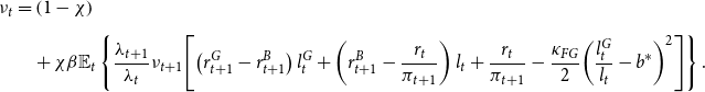 \begin{align} \nu _{t} & =\left (1-\chi \right )\nonumber \\[5pt] &\quad+ \chi \beta \mathbb{E}_{t}\left \{ \frac{\lambda _{t+1}}{\lambda _{t}}\nu _{t+1}\!\left [\left (r_{t+1}^{G}-r_{t+1}^{B}\right )l_{t}^{G}+\left (r_{t+1}^{B}-\frac{r_{t}}{\pi _{t+1}}\right )l_{t}+\frac{r_{t}}{\pi _{t+1}}-\frac{\kappa _{FG}}{2}\!\left (\frac{l_{t}^{G}}{l_{t}}-b^{*}\right )^{2}\right ]\right \}. \end{align}
We have omitted the $j$
index, as every bank chooses the same
$j$
index, as every bank chooses the same $l_t (j )$
and
$l_t (j )$
and $l_t^G (j )$
.Footnote
10
After combining equations (28)–(30) and linearizing around the steady state, we get the following conditions:
$l_t^G (j )$
.Footnote
10
After combining equations (28)–(30) and linearizing around the steady state, we get the following conditions:
 \begin{align} \tilde{l}_{t}&=\eta _{L}\tilde{l}_{t+1}+\beta \!\left [r^{B}l^{B}\!\left (\tilde{r}_{t+1}^{B}-\tilde{rr}_{t}\right )+r^{G}l^{G}\!\left (\tilde{r}_{t+1}^{G}-\tilde{rr}_{t}\right )\right ] \end{align}
 \begin{align} \tilde{b}_{Ft}^{G}-\tilde{b}_{Ft} &=\eta r^G\mathbb{E}_t\!\left (\tilde{r}_{t+1}^{G}-\tilde{r}_{t+1}^{B}\right ), \end{align}
where $\eta _L\equiv \chi \!\left (\frac{l\theta }{\nu }\right )^{2}$
,
$\eta _L\equiv \chi \!\left (\frac{l\theta }{\nu }\right )^{2}$
, $\eta \equiv \frac{l^2}{\kappa _{FG}l^G}$
, and variables without time subscript denote the steady-state value. Equation (31) breaks the interest parity condition between bank’s assets and liabilities: the bank increases its leverage to invest more in green and brown bonds when the lending spreads are expected to be higher. Equation (32) breaks the parity condition within assets: if
$\eta \equiv \frac{l^2}{\kappa _{FG}l^G}$
, and variables without time subscript denote the steady-state value. Equation (31) breaks the interest parity condition between bank’s assets and liabilities: the bank increases its leverage to invest more in green and brown bonds when the lending spreads are expected to be higher. Equation (32) breaks the parity condition within assets: if $\eta \lt \infty$
(i.e. if
$\eta \lt \infty$
(i.e. if $\kappa _{FG}\gt 0$
), an increase in the spread between green and brown bonds induces banks to replace brown bonds with green bonds. Given that changing asset composition is costly, arbitrage does not necessarily bring back the spread to zero. Specifically, parameter
$\kappa _{FG}\gt 0$
), an increase in the spread between green and brown bonds induces banks to replace brown bonds with green bonds. Given that changing asset composition is costly, arbitrage does not necessarily bring back the spread to zero. Specifically, parameter $\eta$
gives the percentage increase in the share of green assets out of total banking assets after a 100 basis points increase in the expected spread between green and brown bonds.
$\eta$
gives the percentage increase in the share of green assets out of total banking assets after a 100 basis points increase in the expected spread between green and brown bonds.
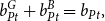
Aggregate net worth can be split between net worth of new bankers $n_{yt}$
and net worth of old bankers
$n_{yt}$
and net worth of old bankers $n_{ot}$
:
$n_{ot}$
:
 \begin{equation*} n_{t}=n_{ot}+n_{yt}. \end{equation*}
Given that a fraction $\chi$
of bankers in period
$\chi$
of bankers in period $t-1$
survive until period
$t-1$
survive until period $t$
, it holds:
$t$
, it holds:
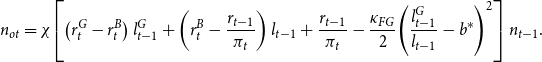 \begin{align} n_{ot}&=\chi \!\left [\left (r_{t}^{G}-r_{t}^{B}\right )l_{t-1}^{G}+\left (r_{t}^{B}-\frac{r_{t-1}}{\pi _{t}}\right )l_{t-1}+\frac{r_{t-1}}{\pi _{t}}-\frac{\kappa _{FG}}{2}\!\left (\frac{l_{t-1}^{G}}{l_{t-1}}-b^{*}\right )^{2}\right ]n_{t-1}. \end{align}
We assume that households transfer a share of assets of exiting bankers $\frac{\iota }{1-\chi }$
to new bankers, in order to start business:
$\frac{\iota }{1-\chi }$
to new bankers, in order to start business:
 \begin{equation} n_{yt}=\iota b_{Ft}. \end{equation}
Using (33) and (34), we can derive an expression for the evolution of aggregate bank net worth:
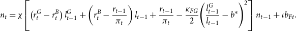 \begin{align} n_{t}&=\chi \!\left [\left (r_{t}^{G}-r_{t}^{B}\right )l_{t-1}^{G}+\left (r_{t}^{B}-\frac{r_{t-1}}{\pi _{t}}\right )l_{t-1}+\frac{r_{t-1}}{\pi _{t}}-\frac{\kappa _{FG}}{2}\!\left (\frac{l_{t-1}^{G}}{l_{t-1}}-b^{*}\right )^{2}\right ]n_{t-1}+\iota b_{Ft}. \end{align}
2.7. Pollution externality
In order to capture the production effects on climate change, we adopt the setup in Heutel (Reference Heutel2012), which merges the baseline RBC model with a simplified version of Nordhaus (Reference Nordhaus2008). In the last version of the Dynamic Integrated model of Climate and the Economy (DICE) by William Nordhaus,Footnote
11
the geophysical sector is linked to the economy as follows. Industrial $\textrm{CO}_2$
emissions are an increasing function of production. Higher emissions increase carbon in the atmosphere, which is also fueled by carbon in the oceans and exogenous non-industrial emissions. Higher values of atmospheric carbon raise the mean surface temperature, which in turn reduces total factor productivity.Footnote
12
$\textrm{CO}_2$
emissions are an increasing function of production. Higher emissions increase carbon in the atmosphere, which is also fueled by carbon in the oceans and exogenous non-industrial emissions. Higher values of atmospheric carbon raise the mean surface temperature, which in turn reduces total factor productivity.Footnote
12
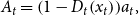
Following Nordhaus (Reference Nordhaus2008), we assume that total factor productivity in green and brown sectors is given by the following expression:
 \begin{equation} A_t=\left (1-D_t\!\left (x_t\right )\right )\!a_t, \end{equation}
where $a_t$
is the exogenous component of TFP and follows an autoregressive process:
$a_t$
is the exogenous component of TFP and follows an autoregressive process:
 \begin{equation} \log \!\left (a_{t}\right )=\left (1-\rho _{a}\right )\log \!\left (\overline{a}\right )+\rho _{a}\log \!\left (a_{t-1}\right )+v_{t}^{a}, \end{equation}
and $v_{t}^{a}\sim N (0,\sigma _{a}^{2} )$
is a technology shock.
$v_{t}^{a}\sim N (0,\sigma _{a}^{2} )$
is a technology shock. $D_t (x_t )$
is the damage function, which is increasing in atmospheric carbon (pollution)
$D_t (x_t )$
is the damage function, which is increasing in atmospheric carbon (pollution) $x_t$
. We model the damage function as follows:
$x_t$
. We model the damage function as follows:
 \begin{equation} D_t=D_0+D_1x_t+D_2x_t^2. \end{equation}
In the DICE model, the output damage is a function of the mean surface temperature, which in turn depends on atmospheric carbon. Compared to the DICE model, in our setting, the output damage is a function of atmospheric carbon only: we follow Heutel (Reference Heutel2012) and Gibson and Heutel (Reference Gibson and Heutel2020), which simplify the damage function by using a formulation as in equation (38), estimating its parameters using the DICE model.
Atmospheric carbon is a stock variable that is fueled by carbon emissions in the domestic economy ( $e_t$
) and in the rest of the world (
$e_t$
) and in the rest of the world ( $e^{\textrm{row}}$
):
$e^{\textrm{row}}$
):
 \begin{equation} x_t=\left (1-\delta _x\right )x_{t-1}+e_t+e^{\textrm{row}}. \end{equation}
Domestic emissions are an increasing and concave function of brown production, as estimated by Heutel (Reference Heutel2012):
 \begin{equation} e_t=\left (y_t^B\right )^{1-\psi }. \end{equation}
2.8. Policy
As before, variables without time subscript denote the steady-state level. We assume that investment in private assets by the central bank is financed through monetary base $b_{Pt}$
:
$b_{Pt}$
:
 \begin{equation} b_{Pt}^{G}+b_{Pt}^{B}=b_{Pt}, \end{equation}
where $b_{Pt}^{G}$
and
$b_{Pt}^{G}$
and $b_{Pt}^{B}$
are green and brown bonds held by the public sector. A constant public consumption
$b_{Pt}^{B}$
are green and brown bonds held by the public sector. A constant public consumption $g$
is financed through lump-sum taxes
$g$
is financed through lump-sum taxes $t_t$
and intermediation profits from the central bank, which transfers its gains to the government:
$t_t$
and intermediation profits from the central bank, which transfers its gains to the government:
 \begin{equation} g =t_{t}+\left (r_{t}^{G}-\frac{r_{t-1}}{\pi _{t}}\right )b_{{Pt}-1}^{G}+\left (r_{t}^{B}-\frac{r_{t-1}}{\pi _{t}}\right )b_{{Pt}-1}^{B}. \end{equation}
There are three policy instruments. The first instrument is the nominal interest rate, set according to a standard Taylor rule:
 \begin{equation} \frac{r_{t}}{r}=\left (\frac{r_{t-1}}{r}\right )^{\rho _{r}}\!\left (\frac{\pi _{t}}{\overline{\pi }}\right )^{\phi _{\pi }\left (1-\rho _{r}\right )}, \end{equation}
where $\overline{\pi }$
is the inflation target. The second instrument is
$\overline{\pi }$
is the inflation target. The second instrument is $b_{Pt}$
, the amount of bonds held by the central bank. We use the following autoregressive rule, which can be interpreted as QE policy:
$b_{Pt}$
, the amount of bonds held by the central bank. We use the following autoregressive rule, which can be interpreted as QE policy:
 \begin{equation} \frac{b_{Pt}}{\bar{b}_P}=\left (\frac{b_{Pt-1}}{\bar{b}_P}\right )^{\rho _{q}}\exp\!\left (v_{t}^{\textrm{qe}}\right ), \end{equation}
where $\bar{b}_P$
denotes the steady-state amount of corporate bonds held by the central bank and
$\bar{b}_P$
denotes the steady-state amount of corporate bonds held by the central bank and $v_{t}^{\textrm{qe}}\sim N (0,\sigma _{\textrm{qe}}^{2})$
is a QE shock.
$v_{t}^{\textrm{qe}}\sim N (0,\sigma _{\textrm{qe}}^{2})$
is a QE shock.
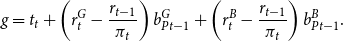
The third instrument is Green QE. Define $\mu _{t}^{G}\equiv \frac{b_{Pt}^{G}}{b_{Pt}}$
as the share of green bonds held by the central bank. Green QE is set according to the following rule:
$\mu _{t}^{G}\equiv \frac{b_{Pt}^{G}}{b_{Pt}}$
as the share of green bonds held by the central bank. Green QE is set according to the following rule:
 \begin{equation} \frac{\mu _{t}^{G}}{\bar{\mu }^{G}}=\left (\frac{\mu _{t-1}^{G}}{\bar{\mu }^{G}}\right )^{\rho _{G}}\!\left [\left (\frac{e_{t}}{e}\right )^{\phi _{G}}\right ]^{1-\rho _{G}}\exp\!\left (v_{t^{\textrm{gqe}}}\right ), \end{equation}
where $\bar{\mu }^{G}$
is the steady-state share and
$\bar{\mu }^{G}$
is the steady-state share and $v_{t}^{\textrm{qe}}\sim N (0,\sigma _{\textrm{qe}}^{2})$
is a Green QE shock. The rule responds to the negative externality generated by the brown sector: when emissions are high relatively to the steady state, the public sector buys green bonds and sell brown bonds.
$v_{t}^{\textrm{qe}}\sim N (0,\sigma _{\textrm{qe}}^{2})$
is a Green QE shock. The rule responds to the negative externality generated by the brown sector: when emissions are high relatively to the steady state, the public sector buys green bonds and sell brown bonds.
We are assuming that the government does not enact any environmental regulation. This may seem odd, as the government is the main responsible for environmental policies. However, in this way we better isolate the role of Green QE. In a follow-up paper, we also show that a carbon tax reduces the effectiveness of Green QE, breaking the link between brown production and emissions, as firms would spend in abatement [Ferrari and Nispi Landi (Reference Ferrari and Nispi Landi2022); see also Abiry et al. (Reference Abiry, Ferdinandusse, Ludwig and Nerlich2022)]. Alternatively, in a cap-and-trade system, emissions would be constrained by the amount of permits distributed: under this system, Green QE would not reduce emissions at all. Given that our findings point out a very limited effectiveness of Green QE, our assumptions are on the conservative side: introducing environmental regulation would strengthen our results, limiting the prospect of green QE even further.
2.9. Market clearing
To close the model, we impose clearing in capital, labor, bond, and good markets. Clearing in capital and labor markets read:
 \begin{align} k_t &= k_t^G+k_t^B \end{align}
 \begin{align} h_t &= h_t^G+h_t^B. \end{align}
Clearing in the bond market:
 \begin{align} b_t^G = b_{Ft}^G+ b_{Ft}^G \end{align}
 \begin{align} b_t^B = b_{Ft}^B+ b_{Pt}^B. \end{align}
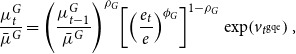
Clearing in the good market implies that final output is consumed either by households or by the government, is invested, and is used to pay price and portfolio adjustment costs:Footnote 13
 \begin{equation} y_{t}=c_{t}+i_{t}+g+\frac{\kappa _{P}}{2}\!\left (\pi _{t}-\overline{\pi }\right )^{2}y_{t}+\frac{\kappa _{FG}}{2}\!\left (\frac{l_{t-1}^{G}}{l_{t-1}}-b^{*}\right )^{2}n_{t-1}. \end{equation}
Finally, we define the following spreads:
 \begin{align} sp_{t}^{G} & =\mathbb{E}_{t}\!\left [r_{t+1}^{G}-\frac{r_{t}}{\pi _{t+1}}\right ] \end{align}
 \begin{align} sp_{t}^{B} & =\mathbb{E}_{t}\!\left [r_{t+1}^{B}-\frac{r_{t}}{\pi _{t+1}}\right ] \end{align}
 \begin{align} sp_{t}^{GB} & =\mathbb{E}_{t}\!\left [r_{t+1}^{G}-r_{t+1}^{B}\right ]. \end{align}
2.10. Calibration
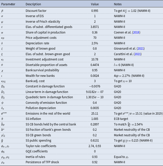
The model is calibrated at the quarterly frequency for the euro area. The euro area is a region that consists of heterogeneous countries, which feature different emissions profiles and economic structures. For the sake of simplicity, we follow most of the literature, and we consider the euro area as a whole. We calibrate most economic and banking parameters following the second version of the New Area-Wide Model [NAWM-II, Coenen et al. (Reference Coenen, Karadi, Schmidt and Warne2018)], an estimated DSGE model for the euro area (Table 1). This simplification comes at the cost of ignoring that environmental policies like Green QE may have different effects on different euro-area countries: how heterogeneous are these effects is a promising topic for future research. We use the following parameters from NAWM-II:
 \begin{equation*} \left \{\alpha,\beta,\sigma,\varphi,\varepsilon,\kappa _P,\delta,\kappa _I,\theta,\chi,\iota,\bar {g},\phi _\pi,\rho _r,\rho _a\right \} \end{equation*}
Some of these parameters are set to match relevant steady-state targets. In particular, following NAWM-II, we calibrate $\beta$
to target a steady-state annualized real interest rate on public liabilities of
$\beta$
to target a steady-state annualized real interest rate on public liabilities of $2\%$
; we calibrate
$2\%$
; we calibrate $\theta$
to get a steady-state bank total leverage of
$\theta$
to get a steady-state bank total leverage of $6$
; we set
$6$
; we set $\iota$
to get an annualized steady-state corporate spread of
$\iota$
to get an annualized steady-state corporate spread of $2.17\%$
; we set
$2.17\%$
; we set $\kappa _P$
to obtain a Calvo parameter of price rigidity equal to
$\kappa _P$
to obtain a Calvo parameter of price rigidity equal to $0.82$
, as in NAWM-II.
$0.82$
, as in NAWM-II.
Table 1. Calibrated parameters. NAWM-II = Coenen et al. (Reference Coenen, Karadi, Schmidt and Warne2018); GH20 = Gibson & Heutel (Reference Gibson and Heutel2020)
Regarding the environmental parameters, we follow Gibson and Heutel (Reference Gibson and Heutel2020), which update the calibration in Heutel (Reference Heutel2012). We assume that the steady-state value of atmospheric carbon $x$
, which is in model units (7644, in our case), corresponds to
$x$
, which is in model units (7644, in our case), corresponds to $x^{GtC}=851$
Gigatons of Carbon (GtC), as in Gibson and Heutel (Reference Gibson and Heutel2020), who follow the 2016 version of the DICE model. Using the same methodology of Gibson and Heutel (Reference Gibson and Heutel2020), we set the parameters of the damage function to
$x^{GtC}=851$
Gigatons of Carbon (GtC), as in Gibson and Heutel (Reference Gibson and Heutel2020), who follow the 2016 version of the DICE model. Using the same methodology of Gibson and Heutel (Reference Gibson and Heutel2020), we set the parameters of the damage function to $D_2= 1.3015e-10$
,
$D_2= 1.3015e-10$
, $D_1= 9.0182e-07$
, and
$D_1= 9.0182e-07$
, and $D_0=-0.0076$
: this implies a steady-state damage of
$D_0=-0.0076$
: this implies a steady-state damage of $0.69\%$
, as in Gibson and Heutel (Reference Gibson and Heutel2020). The elasticity of emissions with respect to output is set to
$0.69\%$
, as in Gibson and Heutel (Reference Gibson and Heutel2020). The elasticity of emissions with respect to output is set to $1-\psi =0.6$
; we set the decay rate of atmospheric carbon to
$1-\psi =0.6$
; we set the decay rate of atmospheric carbon to $1-\delta _x=0.9965$
, which corresponds to a half-life of
$1-\delta _x=0.9965$
, which corresponds to a half-life of $50$
years and follows the estimates of the Fifth Assessment Report of the IPCC; rest-of-the world emissions are 15.3 times larger those of the euro area, which results in
$50$
years and follows the estimates of the Fifth Assessment Report of the IPCC; rest-of-the world emissions are 15.3 times larger those of the euro area, which results in $e^{\textrm{row}}=25.11$
;
$e^{\textrm{row}}=25.11$
;
An important choice is the definition of what is green and what is brown. We follow Carattini et al. (Reference Carattini, Heutel and Melkadze2021) and Giovanardi et al. (Reference Giovanardi, Kaldorf, Radke and Wicknig2021) and interpret $y^G$
and
$y^G$
and $y^B$
as different energy sources. Following Carattini et al. (Reference Carattini, Heutel and Melkadze2021), we set
$y^B$
as different energy sources. Following Carattini et al. (Reference Carattini, Heutel and Melkadze2021), we set $\xi =2$
, implying that the green and the brown goods are imperfect substitutes; we set the weight of the brown good
$\xi =2$
, implying that the green and the brown goods are imperfect substitutes; we set the weight of the brown good $\zeta$
to
$\zeta$
to $0.8$
, as Giovanardi et al. (Reference Giovanardi, Kaldorf, Radke and Wicknig2021), who target the renewable energy share in Europe in 2018.
$0.8$
, as Giovanardi et al. (Reference Giovanardi, Kaldorf, Radke and Wicknig2021), who target the renewable energy share in Europe in 2018.
Regarding the policy parameters, the steady-state inflation target $\bar{\pi }$
is set to
$\bar{\pi }$
is set to $1.005$
, which corresponds to
$1.005$
, which corresponds to $2\%$
yearly. As of November 2021, the ECB holds around 303 Euro billion of corporate bonds in its Corporate Sector Purchase Programme portfolio, which corresponds to
$2\%$
yearly. As of November 2021, the ECB holds around 303 Euro billion of corporate bonds in its Corporate Sector Purchase Programme portfolio, which corresponds to $2.54\%$
of euro-area GDP: we target this latter value to calibrate
$2.54\%$
of euro-area GDP: we target this latter value to calibrate $\bar{b}_P$
. We assume that the central bank’s portfolio is market neutral; hence, the share of green bonds out of total bonds held by the central bank is set to
$\bar{b}_P$
. We assume that the central bank’s portfolio is market neutral; hence, the share of green bonds out of total bonds held by the central bank is set to $0.20$
, the market share. This implies that also the private share of green bonds
$0.20$
, the market share. This implies that also the private share of green bonds $b^*$
is equal to
$b^*$
is equal to $0.20$
. We set the inertia of the QE and the Green QE rules equal to that of the interest rate rule. Our baseline calibration of
$0.20$
. We set the inertia of the QE and the Green QE rules equal to that of the interest rate rule. Our baseline calibration of $\phi _G$
is equal to 0, but we perform some simulations with positive values for this parameters.
$\phi _G$
is equal to 0, but we perform some simulations with positive values for this parameters.
An important parameter is the value of the adjustment cost of the banking sector, $\kappa _{FG}$
, which measures the costs of arbitraging between green and brown bonds. The main message of our paper is that Green QE has small effects: to be conservative, we set this parameter to a high value, in order to maximize the potential effects of Green QE. Specifically, we assume that a reduction of 100 basis points in the spread between green and brown rates leads banks to reduce green bonds by
$\kappa _{FG}$
, which measures the costs of arbitraging between green and brown bonds. The main message of our paper is that Green QE has small effects: to be conservative, we set this parameter to a high value, in order to maximize the potential effects of Green QE. Specifically, we assume that a reduction of 100 basis points in the spread between green and brown rates leads banks to reduce green bonds by $10\%$
, keeping constant total bonds (see equation 32): we set
$10\%$
, keeping constant total bonds (see equation 32): we set $\kappa _{FG}=3$
in order to have
$\kappa _{FG}=3$
in order to have $\eta =10$
. This arbitrage opportunity is in the higher end of estimates found in the literature.Footnote
14
In some experiments, we set
$\eta =10$
. This arbitrage opportunity is in the higher end of estimates found in the literature.Footnote
14
In some experiments, we set $\eta =0$
(infinite adjustment costs) for illustrative purposes.
$\eta =0$
(infinite adjustment costs) for illustrative purposes.
3. Temporary Green QE
In our baseline model, we can only study a transitory Green QE. A permanent Green QE has no effects on economic activity in the long run, because in the steady-state adjustment costs are 0 by definition and Wallace neutrality holds: if the central bank increases the share of green bonds in its portfolio permanently, in the new steady-state banks decrease the share of brown bonds, with any effect on relative returns. Moreover, in our model a permanent Green QE has no short-run effects either: banks immediately jump to the new steady state, in order to avoid to pay adjustment costs, as the latter are defined relatively to the steady-state share of green bonds.
In this section, we simulate several scenarios to study the positive and normative properties of a transitory Green QE. First, we simulate a Green QE shock, which does not change the size of the central bank’s balance sheets. Second, we simulate a Green QE shock that increases the size of the central bank’s balance sheets. Third, we study a Green QE rule in response to a TFP shock, quantifying its welfare gains.
These exercises are based on a first-order approximation of the model around the deterministic steady state.Footnote 15 This may seem at odds with empirical evidence, as CO2 emissions grow over time. One potential solution could be adding exogenous trend growth, finding the steady-state growth path, and then detrending all variables. Under the assumption that pollution does not affect TFP, this amendment would be straightforward, results would be barely affected, and pollution would grow over time. Instead, the assumptions of a pollution damage function plus exogenous TFP growth would greatly complicate the model. Moreover, one could still argue that the climate is not in a steady-state growth path either, but along the transition to it. However, as suggested by Heutel (Reference Heutel2012), if the economy is not currently in a steady state nor in a steady-state growth path, an environmental model with a constant steady state is still able to give policy recommendations right now, under the assumption that cycles around the transition behaves the same as cycles around the future steady-state growth path. This seems a reasonable assumption for most economic parameters. Regarding the environmental parameters, in the new steady-state pollution damage is likely to be higher: in the sensitivity analysis, we study Green QE assuming a larger steady-state damage.Footnote 16
3.1. When Green QE is effective
We simulate the effects of a Green QE shock ( $v_t^\textrm{gqe}=4$
) such that the central bank sells all the brown bonds in its portfolio, to buy green bonds: the size of central bank’s balance sheet is kept at the steady state, meaning that the investment in green bonds is entirely financed through a reduction in brown bonds. The increase in central bank’s green bond is persistent but not permanent, as specified by equation (45). We plot the impulse response functions for three different values of
$v_t^\textrm{gqe}=4$
) such that the central bank sells all the brown bonds in its portfolio, to buy green bonds: the size of central bank’s balance sheet is kept at the steady state, meaning that the investment in green bonds is entirely financed through a reduction in brown bonds. The increase in central bank’s green bond is persistent but not permanent, as specified by equation (45). We plot the impulse response functions for three different values of $\eta$
, which is the elasticity of the green-brown bond demand with respect to the green-brown spread:
$\eta$
, which is the elasticity of the green-brown bond demand with respect to the green-brown spread: $\infty$
(blue solid line, Figure 1), 10 (red dotted line, Figure 1),
$\infty$
(blue solid line, Figure 1), 10 (red dotted line, Figure 1), $0$
(black dashed line, Figure 1). If
$0$
(black dashed line, Figure 1). If $\eta \rightarrow \infty$
, banks do not pay adjustment costs when they change their asset composition (
$\eta \rightarrow \infty$
, banks do not pay adjustment costs when they change their asset composition ( $\kappa _{FG}=0$
): green and brown bonds are perfect substitutes, the central bank is not able to affect the interest rates on these bonds. The increase in green bonds held by the central bank is fully offset by the reduction of green bonds held by private banks. The irrelevance of Green QE when green and brown bonds are perfect substitutes occurs even in a model where QE is able to affect the real economy.
$\kappa _{FG}=0$
): green and brown bonds are perfect substitutes, the central bank is not able to affect the interest rates on these bonds. The increase in green bonds held by the central bank is fully offset by the reduction of green bonds held by private banks. The irrelevance of Green QE when green and brown bonds are perfect substitutes occurs even in a model where QE is able to affect the real economy.
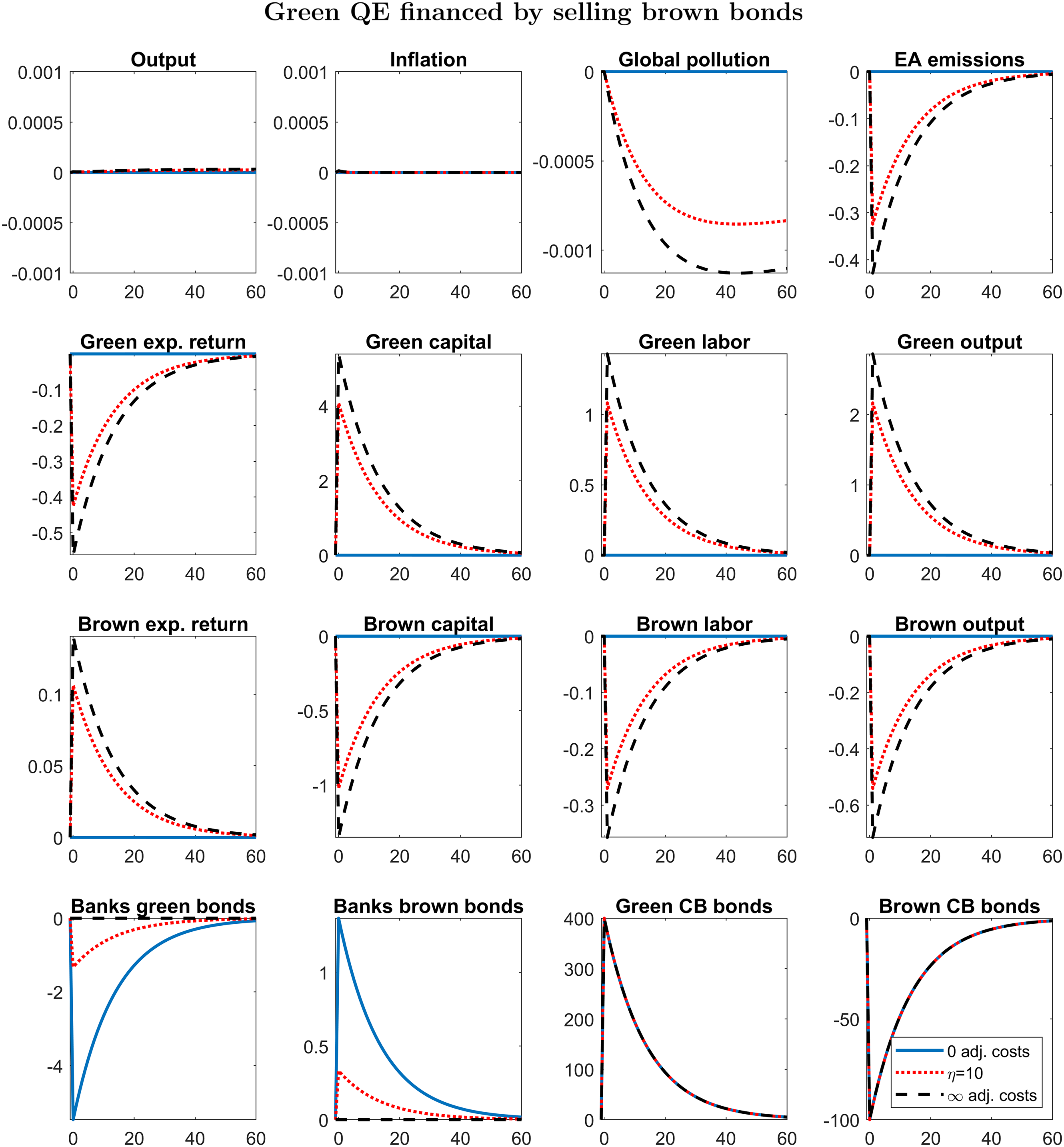
Figure 1. IRFs to a GQE shock that sells all brown bonds in the central bank’s balance sheets on impact. Responses are in log deviations from the steady state, except for inflation and returns, whose responses are in quarterly percent deviations from the steady state reported at annual rates. Blue solid line: $\eta \rightarrow \infty$
(no adjustment cost). Red dotted line:
$\eta \rightarrow \infty$
(no adjustment cost). Red dotted line: $\eta =10$
. Black dashed line:
$\eta =10$
. Black dashed line: $\eta =0$
(infinite adjustment costs).
$\eta =0$
(infinite adjustment costs).
If green and brown bonds are not perfect substitutes, Green QE does have an effect on macroeconomic and environmental variables. The increase in green bonds held by the central bank reduces (increases) the interest rate paid by green (brown) firms. Even if brown bonds pay a higher interest rate, banks do not fully exploit the arbitrage opportunity, because changing the asset composition is costly. Capital expenses are lower for green firms, which rent more capital and produce more. The opposite holds for brown firms, which reduce production.
From a quantitative point of view, the impact of green QE is relatively small. Even in the scenario with infinite adjustment costs ( $\eta =0$
, black solid line in Figure 1), euro-area emissions fall on impact by
$\eta =0$
, black solid line in Figure 1), euro-area emissions fall on impact by $0.4\%$
, and they come back to the steady state after some years, given that the shock is transitory. The fall in atmospheric carbon is 2–3 orders of magnitude smaller and much more persistent.
$0.4\%$
, and they come back to the steady state after some years, given that the shock is transitory. The fall in atmospheric carbon is 2–3 orders of magnitude smaller and much more persistent.
Why does Green QE have small effects on atmospheric carbon? The economic intuition is the following. In our model, atmospheric carbon follows an extremely persistent law of motion. As a result, the initial stock of atmospheric carbon is two orders of magnitude larger than the flow of total emissions (domestic plus rest of the world). Moreover, the euro area contributes only to $6.5\%$
of world emissions: it turns out that the initial stock of atmospheric carbon is three orders of magnitude larger than euro-area emissions: even large changes in the emission flow have small effects on the pollution stock on impact. If we consider the impact on euro-area driven pollution, at the peak the impact of Green QE is around
$6.5\%$
of world emissions: it turns out that the initial stock of atmospheric carbon is three orders of magnitude larger than euro-area emissions: even large changes in the emission flow have small effects on the pollution stock on impact. If we consider the impact on euro-area driven pollution, at the peak the impact of Green QE is around $0.02\%$
, with infinite adjustment costs.
$0.02\%$
, with infinite adjustment costs.
Why does Green QE seem not effective on total output and inflation? In principles, Green QE may affect aggregate variables either by increasing TFP via a lower pollution, or by a composition effect, shifting resources from the brown to the green sector.
The TFP channel is almost irrelevant for the following reason. The damage function yields a steady-state output loss of only $0.7\%$
. The low steady-state output loss also implies a low first derivative of damage with respect to pollution, given the convexity of the TFP function.Footnote
17
The combination of a low effect of euro-area emissions on the pollution stock (as explained in the previous paragraph) and a low effect of pollution on TFP explains why the TFP channel is almost irrelevant: in order to highlight this concept, in Figure 1 we set the range of the impulse response functions of output and inflation to
$0.7\%$
. The low steady-state output loss also implies a low first derivative of damage with respect to pollution, given the convexity of the TFP function.Footnote
17
The combination of a low effect of euro-area emissions on the pollution stock (as explained in the previous paragraph) and a low effect of pollution on TFP explains why the TFP channel is almost irrelevant: in order to highlight this concept, in Figure 1 we set the range of the impulse response functions of output and inflation to $\pm 0.001\%$
: to be precise, in Figure 1 the peak response of output is
$\pm 0.001\%$
: to be precise, in Figure 1 the peak response of output is $3.3\times 10^{-5}\%$
, when adjustment costs are infinite. In Section 5.2, we consider a higher steady-state damage.
$3.3\times 10^{-5}\%$
, when adjustment costs are infinite. In Section 5.2, we consider a higher steady-state damage.
The composition channel is 0 under our calibration: absent the TFP channel, the increase in green output would be fully offset by the reduction in brown output. This result would change if we relax the assumption of equal capital share in the production function.Footnote 18
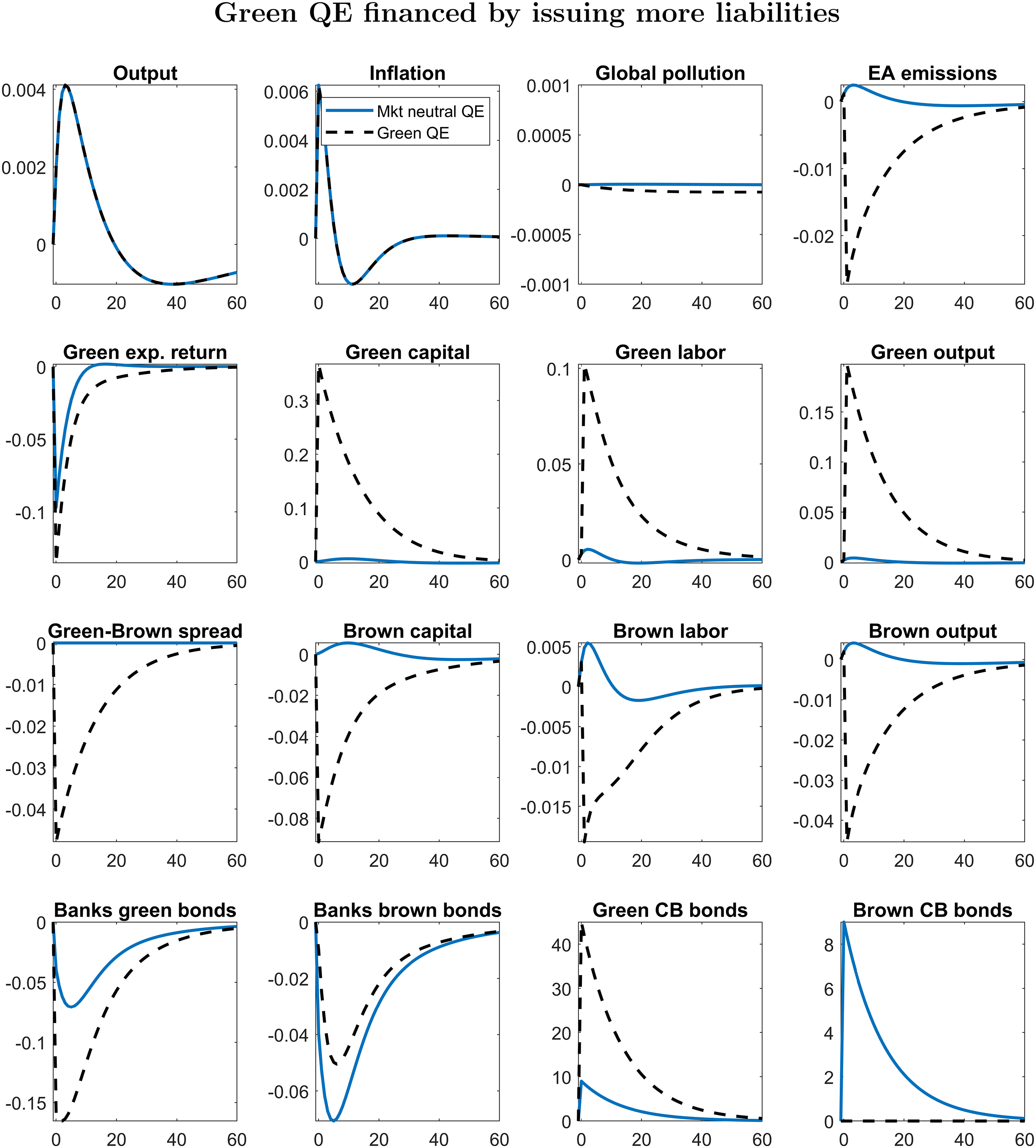
Figure 2. IRFs to a 9% positive QE shock. Responses are in log deviations from the steady state, except for inflation, returns, and spreads, whose responses are in quarterly percent deviations from the steady state reported at annual rates. Blue solid line: the composition of green and brown bonds in central bank’s balance sheet does not change. Black dashed line: QE is entirely targeted to green bonds.
Finally, we highlight that the response of green and brown labor crucially depends on the elasticity of intratemporal substitution $\xi$
. Combining equations (7), (8), (14), and (17), and linearizing we get:
$\xi$
. Combining equations (7), (8), (14), and (17), and linearizing we get:
 \begin{equation} \tilde{h}_{t}^{G}-\tilde{h}_{t}^{B}=\left (1-\xi \right )\left (\tilde{p}_{t}^{G}-\tilde{p}_{t}^{B}\right ). \end{equation}
Green QE increases the marginal cost of brown firms, and the marginal product has to rise accordingly: the price of brown firms is higher. The opposite holds for green firms, and the response of the green-brown relative price $ (\tilde{p}_{t}^{G}-\tilde{p}_{t}^{B} )$
is negative after a Green QE shock. The effect on the relative labor demand depends on two channels. First, a lower green-brown relative price decreases the labor demand of green firms and increases that of brown firms. Second, a lower green-brown relative price increases the green input demand of intermediate firms, while decreasing their brown input demand: this channel is more relevant when green and brown goods are substitutes rather than complements, that is when
$ (\tilde{p}_{t}^{G}-\tilde{p}_{t}^{B} )$
is negative after a Green QE shock. The effect on the relative labor demand depends on two channels. First, a lower green-brown relative price decreases the labor demand of green firms and increases that of brown firms. Second, a lower green-brown relative price increases the green input demand of intermediate firms, while decreasing their brown input demand: this channel is more relevant when green and brown goods are substitutes rather than complements, that is when $\xi$
is relatively higher. If
$\xi$
is relatively higher. If $\xi \gt 1$
, as in our calibration, the right-hand side of (54) is positive, green labor rises and brown labor falls. In Section 5.3, we relax the assumption of
$\xi \gt 1$
, as in our calibration, the right-hand side of (54) is positive, green labor rises and brown labor falls. In Section 5.3, we relax the assumption of $\xi \gt 1$
.
$\xi \gt 1$
.
3.2. A green increase in central bank’s balance sheets
At the end of 2020, the ECB has increased its stock of corporate bonds by $36\%$
compared to the end of 2019: this corresponds to a quarterly increase of approximately
$36\%$
compared to the end of 2019: this corresponds to a quarterly increase of approximately $9\%$
. We simulate the effects of a
$9\%$
. We simulate the effects of a $9\%$
temporary increase in central bank’s assets (
$9\%$
temporary increase in central bank’s assets ( $v_t^{\textrm{qe}}=0.09$
), comparing two scenarios. In the first scenario, the central bank does not change the asset composition: QE is market neutral (blue solid line, Figure 2), because the intervention does not affect the spread between green and brown bonds. This policy puts downward pressure on the expected interest rate paid by green and brown firms, which both raise physical capital and labor, stimulating production: emission and pollution slightly rise. Banks reduce investment in green and brown firms, in response to lower lending rates. Total output rises, driving inflationary pressures.
$v_t^{\textrm{qe}}=0.09$
), comparing two scenarios. In the first scenario, the central bank does not change the asset composition: QE is market neutral (blue solid line, Figure 2), because the intervention does not affect the spread between green and brown bonds. This policy puts downward pressure on the expected interest rate paid by green and brown firms, which both raise physical capital and labor, stimulating production: emission and pollution slightly rise. Banks reduce investment in green and brown firms, in response to lower lending rates. Total output rises, driving inflationary pressures.
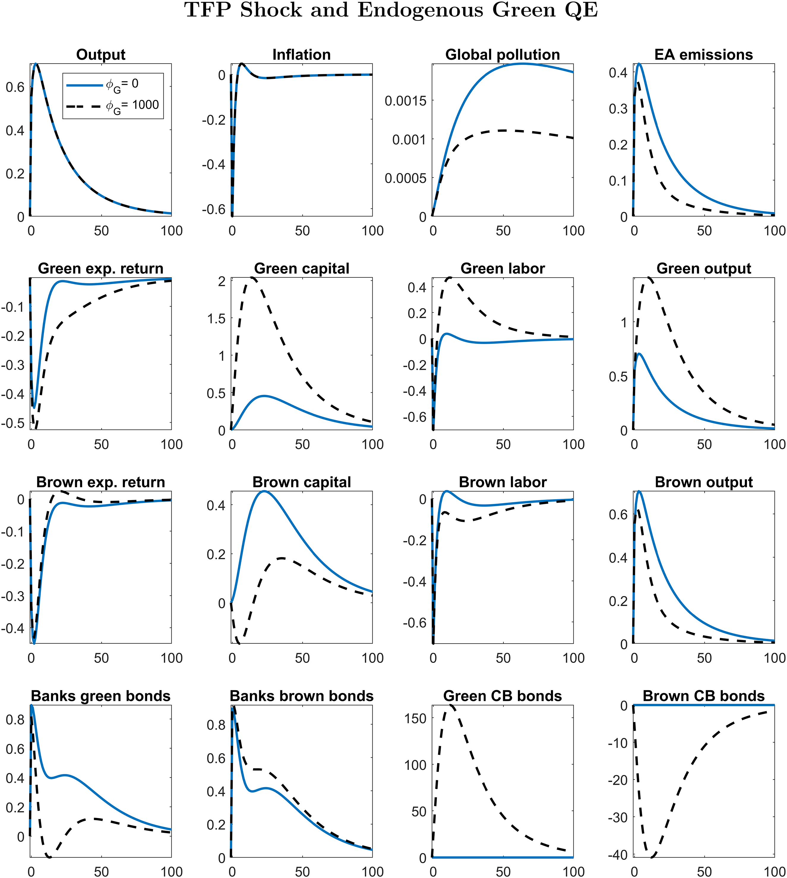
Figure 3. IRFs to a 1% positive TFP shock. Responses are in log deviations from the steady state, except for inflation and returns, whose responses are in quarterly percent deviations from the steady state reported at annual rates. Blue solid line: Green QE does not respond. Black dashed line: Green QE responds to emissions with $\phi _G=1000$
.
$\phi _G=1000$
.
In the second scenario, the intervention is entirely targeted to green bonds (black dotted line, Figure 2): this is a Green QE that increases the size of the central bank’s balance sheet. We replace the Green QE rule [equation (45)] with $b_{Pt}^B=b_{P}^B$
: brown bonds held by the central bank remain in the steady state. Unlike the simulation in Figure 1 where the size of central bank’s assets is kept constant, the increase in green bonds is not offset by a reduction in brown bonds, but it is financed with higher liabilities. When brown and green bonds are imperfect substitutes (
$b_{Pt}^B=b_{P}^B$
: brown bonds held by the central bank remain in the steady state. Unlike the simulation in Figure 1 where the size of central bank’s assets is kept constant, the increase in green bonds is not offset by a reduction in brown bonds, but it is financed with higher liabilities. When brown and green bonds are imperfect substitutes ( $\eta = 10$
), the spread between green and brown expected returns slightly decreases. Banks sell green and buy brown bonds, but not enough to offset the central bank’s intervention: brown firms face higher capital costs and reduce capital demand and production. The intervention is able to slightly increase production and to shift resources from the brown to the green sectors, given that under our calibration the brown and the green good are imperfect substitutes. The fall in euro-area emissions is again quite modest, around 0.025% at the peak. The fall in pollution is negligible. With regard to aggregate macroeconomic variables, the difference between the two scenarios is in fact invisible: this is the result of the tiny effects of Green QE, highlighted in Figure 1.
$\eta = 10$
), the spread between green and brown expected returns slightly decreases. Banks sell green and buy brown bonds, but not enough to offset the central bank’s intervention: brown firms face higher capital costs and reduce capital demand and production. The intervention is able to slightly increase production and to shift resources from the brown to the green sectors, given that under our calibration the brown and the green good are imperfect substitutes. The fall in euro-area emissions is again quite modest, around 0.025% at the peak. The fall in pollution is negligible. With regard to aggregate macroeconomic variables, the difference between the two scenarios is in fact invisible: this is the result of the tiny effects of Green QE, highlighted in Figure 1.
3.3. A Green QE rule
3.3.1. Positive analysis
What is the role of Green QE in mitigating emissions during expansion periods? We simulate the effects of an exogenous $1\%$
increase in TFP and compare two scenarios.
$1\%$
increase in TFP and compare two scenarios.
In the first scenario, the Green QE rule is off [ $\phi _{G}=0$
in equation (45)]. The effect of the TFP shock is standard (blue solid line, Figure 3). Economic activity expands. Inflation falls as a result of higher supply. Banking profits rise and the increase in net worth is higher than the increase in lending: the leverage ratio is lower, lending rates fall. The increase in TFP is common to green and brown sectors: emissions and pollution grow.
$\phi _{G}=0$
in equation (45)]. The effect of the TFP shock is standard (blue solid line, Figure 3). Economic activity expands. Inflation falls as a result of higher supply. Banking profits rise and the increase in net worth is higher than the increase in lending: the leverage ratio is lower, lending rates fall. The increase in TFP is common to green and brown sectors: emissions and pollution grow.
In the second scenario, we activate the Green QE rule with $\phi _G=1000$
(black dotted line, Figure 3). This arbitrarily large value implies that the central bank sells around
$\phi _G=1000$
(black dotted line, Figure 3). This arbitrarily large value implies that the central bank sells around $40\%$
of its brown bonds stock at the peak. Procyclical Green QE partially mitigates the brown output increase and the resulting emissions. The transmission mechanism is now well understood: banks face a reduction in the green-brown spread and change their portfolio toward brown bonds. This shift does not offset the central bank’s intervention as a result of adjustment costs (we keep
$40\%$
of its brown bonds stock at the peak. Procyclical Green QE partially mitigates the brown output increase and the resulting emissions. The transmission mechanism is now well understood: banks face a reduction in the green-brown spread and change their portfolio toward brown bonds. This shift does not offset the central bank’s intervention as a result of adjustment costs (we keep $\eta =10$
). Brown firms reduce capital, despite the increase in TFP. The rise in capital is amplified for green. We continue to stress that the overall effects of the rule are tiny, despite the large sale of brown bonds by the central bank.
$\eta =10$
). Brown firms reduce capital, despite the increase in TFP. The rise in capital is amplified for green. We continue to stress that the overall effects of the rule are tiny, despite the large sale of brown bonds by the central bank.
3.3.2. Normative analysis
Should the central bank buy green and sell brown bonds, when emissions increase?Footnote
19
In this section, we address this question through the following thought experiment. We numerically search for the Green QE parameter $\phi ^G$
that maximizes the impact response of the following welfare function to a one-standard-deviation positive TFP shock:
$\phi ^G$
that maximizes the impact response of the following welfare function to a one-standard-deviation positive TFP shock:
 \begin{equation} \mathcal{W}_0=\left (\frac{c_{0}^{1-\sigma }}{1-\sigma }-\frac{h_{0}^{1+\varphi }}{1+\varphi }\right )+\beta \mathbb{E}_0 \!\left (\mathcal{W}_{1}\right ). \end{equation}
This exercise is different from the common practice of optimizing simple rules by maximizing welfare conditional on future shocks, both positive and negative. We choose this approach because we see Green QE as a policy tool available during expansion periods only. Otherwise, the central bank should buy brown and sell green bonds during recessions: such a policy would be politically hard to support and ethically questionable. This approach is similar in spirit to Gertler and Karadi (Reference Gertler and Karadi2011)’s welfare analysis: in computing the optimal QE policy, the authors only consider a crisis episode. Similarly, we consider an expansion period in which emissions increase. We find that during a TFP-driven expansion, the central bank should aggressively respond to the emission rise by selling brown bonds and buying green bonds. The optimal $\phi ^G$
is the upper bound of the grid even when the upper bound is higher than
$\phi ^G$
is the upper bound of the grid even when the upper bound is higher than $1e4$
. As in Gertler and Karadi (Reference Gertler and Karadi2011), given that we are simulating a single event, we define the consumption equivalent as the percentage gain in consumption in the first four quarters that would make welfare under no Green QE equal to welfare under optimal Green QE. With
$1e4$
. As in Gertler and Karadi (Reference Gertler and Karadi2011), given that we are simulating a single event, we define the consumption equivalent as the percentage gain in consumption in the first four quarters that would make welfare under no Green QE equal to welfare under optimal Green QE. With $\phi _G=1e4$
, this measure of consumption equivalent is small, around to
$\phi _G=1e4$
, this measure of consumption equivalent is small, around to $0.0025\%$
of steady-state consumption.Footnote
20
The low welfare gain is the result of three features of the model: the low output loss of pollution; the extremely persistent law of motion of atmospheric carbon, whereby a temporary policy such as Green QE is not appropriate; the small impact that euro-area policy can have on global emissions.
$0.0025\%$
of steady-state consumption.Footnote
20
The low welfare gain is the result of three features of the model: the low output loss of pollution; the extremely persistent law of motion of atmospheric carbon, whereby a temporary policy such as Green QE is not appropriate; the small impact that euro-area policy can have on global emissions.
So far, we have not imposing any inefficiency cost from central bank’s intermediation. Following Gertler and Karadi (Reference Gertler and Karadi2011), we introduce a central bank’s intermediation cost, when the central bank changes its portfolio allocation:Footnote 21
 \begin{equation} \textrm{INT}^\textrm{cost}_t=\kappa _\textrm{INT}\!\left |\frac{\mu _t^G}{\bar{\mu }^G}-1\right |. \end{equation}
This formulation captures that the central bank is not as efficient as private banks in intermediating funds. Moreover, we are explicitly modeling that deviating from market neutrality may entail some costs for the central bank. The central bank loses the following basis points for each additional unit of green bonds, sufficiently close to the steady state:Footnote 22
 \begin{equation} \textrm{BP}=10^{4}\kappa _\textrm{INT}\frac{1-\bar{\mu }^{G}}{b_P^G}. \end{equation}
We repeat the normative analysis and find that the optimal parameter in the Green QE rule is greater than 0 only if $\textrm{BP}\,\lt\,0.2$
basis points, a very small value: this implies that Green QE is not welfare improving even when the central bank is only slightly more inefficient than the private sector in intermediating funds.
$\textrm{BP}\,\lt\,0.2$
basis points, a very small value: this implies that Green QE is not welfare improving even when the central bank is only slightly more inefficient than the private sector in intermediating funds.
4. Permanent Green QE
A permanent Green QE is not effective in our baseline model in the long run. We see this as a reasonable feature of our model, which follows the tradition of the New Keynesian literature, where monetary policy is neutral in the long term. In our baseline model, a permanent Green QE would not be effective also in the short-run: in this section, we modify the adjustment-cost function in order to study the short-run effects of a permanent Green QE. We consider a simplified version of the model, where firms issue bonds directly to households, without banking intermediation. We assume that households face an endogenous risk premium when they invest in green and brown bonds. The resulting Euler equations read, for $i=G,B$
:
$i=G,B$
:
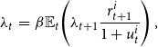 \begin{eqnarray} \lambda _{t}&=&\beta \mathbb{E}_{t}\!\left (\lambda _{t+1}\frac{r_{t+1}^{i}}{1+u_{t}^{i}}\right ), \end{eqnarray}
where $u_t^G$
and
$u_t^G$
and $u_t^B$
are the green and brown premia on the risk-free rate. Following Chen et al. (Reference Chen, Cúrdia and Ferrero2012), we interpret these premia as a cost arising for a loss of liquidity that households hedge by holding more money in their portfolio. These costs are exogenous from the point of view of households and are paid to a non-modeled financial sector. In the same spirit of Chen et al. (Reference Chen, Cúrdia and Ferrero2012), we assume that these premia are increasing in the amount of bonds in the hands of households. We consider the following formulation, for
$u_t^B$
are the green and brown premia on the risk-free rate. Following Chen et al. (Reference Chen, Cúrdia and Ferrero2012), we interpret these premia as a cost arising for a loss of liquidity that households hedge by holding more money in their portfolio. These costs are exogenous from the point of view of households and are paid to a non-modeled financial sector. In the same spirit of Chen et al. (Reference Chen, Cúrdia and Ferrero2012), we assume that these premia are increasing in the amount of bonds in the hands of households. We consider the following formulation, for $i=G,B$
:
$i=G,B$
:
 \begin{eqnarray} u_{t}^{i}&=&u^{i}\!\left [1+\kappa _{Hi}\!\left (\frac{b_{Ft}^{i}}{b_{Ft-1}^{i}}-1\right )\right ], \end{eqnarray}
where $u_i$
is the steady state of
$u_i$
is the steady state of $u_{it}$
, for
$u_{it}$
, for $i=G,B$
;
$i=G,B$
; $\kappa _{HG}$
and
$\kappa _{HG}$
and $\kappa _{HB}$
are parameters calibrated to match a desired bond-elasticity to the green-brown spread. We highlight that this function for the transaction cost does not pin down the steady state of the share of green bonds: a permanent Green QE does have short-run effects, because households take time to reach the new steady state with a lower share of green bonds in their portfolios. However, the private and the central bank’s portfolio allocations are the only variables that change in the new steady state: in the long run, adjustment costs are zero and all the other variables come back to the initial steady state.
$\kappa _{HB}$
are parameters calibrated to match a desired bond-elasticity to the green-brown spread. We highlight that this function for the transaction cost does not pin down the steady state of the share of green bonds: a permanent Green QE does have short-run effects, because households take time to reach the new steady state with a lower share of green bonds in their portfolios. However, the private and the central bank’s portfolio allocations are the only variables that change in the new steady state: in the long run, adjustment costs are zero and all the other variables come back to the initial steady state.
By combining the Euler equations and linearizing around the steady state, we get:
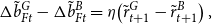 \begin{equation} \Delta \tilde{b}_{Ft}^{G}-\Delta \tilde{b}_{Ft}^{B}=\eta \!\left (\tilde{r}_{t+1}^{G}-\tilde{r}_{t+1}^{B}\right ), \end{equation}
where $\eta \equiv \frac{1+u}{u\kappa _{HG}}$
,
$\eta \equiv \frac{1+u}{u\kappa _{HG}}$
, $\Delta$
denotes a first difference, and we have assumed
$\Delta$
denotes a first difference, and we have assumed $\kappa _{HB}=\kappa _{HG}$
. Equation (60) is the counterpart of equation (32) in the baseline model: when Green QE reduces the spread between green and brown bonds, the private sector takes time to adjust the portfolio allocation, in order to save transaction costs. The lower
$\kappa _{HB}=\kappa _{HG}$
. Equation (60) is the counterpart of equation (32) in the baseline model: when Green QE reduces the spread between green and brown bonds, the private sector takes time to adjust the portfolio allocation, in order to save transaction costs. The lower $\eta$
, the less households adjust the portfolio allocation, and the more Green QE is effective.
$\eta$
, the less households adjust the portfolio allocation, and the more Green QE is effective.
We consider a permanent increase in the share of green bonds held by the central bank such that all brown bonds are sold forever (Figure 4). We analyze three different calibrations for $\eta$
. In the blue solid line,
$\eta$
. In the blue solid line, $\eta =1000$
, a value in line with the elasticity estimated by Chen et al. (Reference Chen, Cúrdia and Ferrero2012).Footnote
23
In the red dotted line
$\eta =1000$
, a value in line with the elasticity estimated by Chen et al. (Reference Chen, Cúrdia and Ferrero2012).Footnote
23
In the red dotted line $\eta =10$
, as in our baseline calibration. In the black dashed line,
$\eta =10$
, as in our baseline calibration. In the black dashed line, $\eta =1$
, an extreme value set for illustrative purpose. Overall, the effects are similar to the one obtained in the baseline model, though they are much more persistent: a permanent Green QE is able to temporarily reduce emissions, but quantitatively the effect is very small.
$\eta =1$
, an extreme value set for illustrative purpose. Overall, the effects are similar to the one obtained in the baseline model, though they are much more persistent: a permanent Green QE is able to temporarily reduce emissions, but quantitatively the effect is very small.
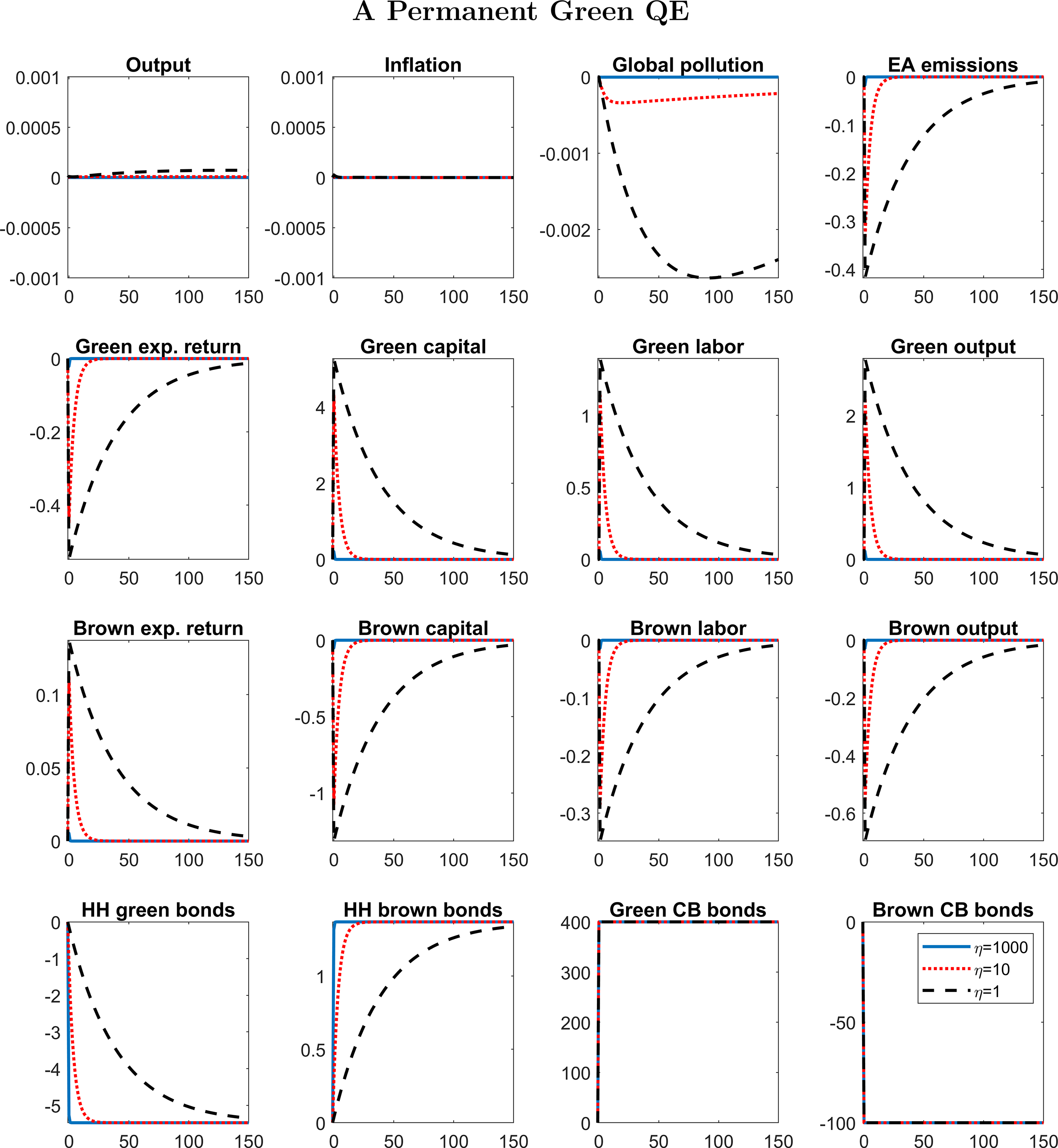
Figure 4. IRFs to a GQE shock that sells all brown bonds in the central bank’s balance sheets forever. Responses are in log deviations from the steady state, except for inflation and returns, whose responses are in quarterly percent deviations from the steady state reported at annual rates. Blue solid line: $\eta =1000$
. Red dotted line:
$\eta =1000$
. Red dotted line: $\eta =10$
. Black dashed line:
$\eta =10$
. Black dashed line: $\eta =1$
.
$\eta =1$
.
5. Sensitivity analysis and additional exercises
In this section, we change some key parameters to explore which ones are key for a more powerful effect of Green QE. In particular, we change the depreciation rate of pollution $\delta ^x$
and the pollution law of motion, the steady-state damage of pollution, and the elasticity of substitution between green and brown goods
$\delta ^x$
and the pollution law of motion, the steady-state damage of pollution, and the elasticity of substitution between green and brown goods $\xi$
. Moreover, we study Green QE in response to an emission shock. We keep infinite adjustment costs throughout the section. The figures are in Online Appendix A.
$\xi$
. Moreover, we study Green QE in response to an emission shock. We keep infinite adjustment costs throughout the section. The figures are in Online Appendix A.
5.1. Pollution depreciation
In our baseline calibration, we assume that the decay rate of CO2 from the atmosphere is geometric. This is a simplification often used in stationary models that study environmental policies at business cycle frequencies.Footnote 24 In reality, the depreciation is faster in the first decades and slower in the very long run, as captured by the environmental models of Golosov et al. (Reference Golosov, Hassler, Krusell and Tsyvinski2014) and Hassler et al. (Reference Hassler, Krusell and Smith2016). We modify our depreciation process as follows:
 \begin{equation} x_t=\left (1-\delta _x\right )x_{t-1}+\gamma \!\left (e_t+e^{\textrm{row}}\right ), \end{equation}
which implies that the share of emissions that remains in the atmosphere after $j$
periods is given by:
$j$
periods is given by: $\gamma (1-\delta _x )^{j}$
. This is equivalent to the depreciation structure in Golosov et al. (Reference Golosov, Hassler, Krusell and Tsyvinski2014) and Hassler et al. (Reference Hassler, Krusell and Smith2016), with a twist: we are imposing that all emissions leave the atmosphere in the very long run, to maintain stationarity.Footnote
25
We transform the calibration in Hassler et al. (Reference Hassler, Krusell and Smith2016) where one period is equal to 10 years into a quarterly calibration: we set
$\gamma (1-\delta _x )^{j}$
. This is equivalent to the depreciation structure in Golosov et al. (Reference Golosov, Hassler, Krusell and Tsyvinski2014) and Hassler et al. (Reference Hassler, Krusell and Smith2016), with a twist: we are imposing that all emissions leave the atmosphere in the very long run, to maintain stationarity.Footnote
25
We transform the calibration in Hassler et al. (Reference Hassler, Krusell and Smith2016) where one period is equal to 10 years into a quarterly calibration: we set $\delta _x=0.0006$
[parameter
$\delta _x=0.0006$
[parameter $\phi$
in Hassler et al. (Reference Hassler, Krusell and Smith2016)] and
$\phi$
in Hassler et al. (Reference Hassler, Krusell and Smith2016)] and $\gamma =0.536$
[parameter
$\gamma =0.536$
[parameter $\phi _0$
in Hassler et al. (Reference Hassler, Krusell and Smith2016)].
$\phi _0$
in Hassler et al. (Reference Hassler, Krusell and Smith2016)].
We plot a Green QE shock comparing a scenario under our baseline depreciation (Figure A.1, blue solid line) with a scenario under the new calibration (Figure A.1, black dashed line). If the depreciation is faster in the first decades, pollution falls by less after Green QE in the first 150 years: under the new calibration, a share of emissions leaves the atmosphere quickly; therefore, the derivative of pollution with respect to emissions is smaller for many years. After about 150 years, the new law of motion implies that Green QE is more effective on pollution, although the overall effect is still negligible.
5.2. Pollution damage
We explore how much results change quantitatively by increasing the pollution TFP damage. We modify the damage function [equation (38)] as follows:
 \begin{equation} D_t=d_3\!\left (D_0+D_1x_t+D_2x_t^2\right ). \end{equation}
We compare the baseline scenario (Figure A.2, blue solid line), with an alternative scenario where $d_3=7.5$
, implying a big steady-state damage (about
$d_3=7.5$
, implying a big steady-state damage (about $5\%$
of TFP) and a higher derivative of TFP damage with respect to pollution (Figure A.2, black dashed line). In the new scenario, the output gain is larger compared to the previous scenarios, but still quite low: at the peak output rises by about
$5\%$
of TFP) and a higher derivative of TFP damage with respect to pollution (Figure A.2, black dashed line). In the new scenario, the output gain is larger compared to the previous scenarios, but still quite low: at the peak output rises by about $0.0003\%$
(Figure A.2, red dotted line), compared to the baseline calibration (blue solid line). Other variables are barely affected.
$0.0003\%$
(Figure A.2, red dotted line), compared to the baseline calibration (blue solid line). Other variables are barely affected.
5.3. Varying the elasticity of substitution
In the baseline specification, the elasticity of substitution $\xi$
between green and brown goods in the production function is equal to
$\xi$
between green and brown goods in the production function is equal to $2$
, meaning that green and brown goods are imperfect substitutes: this is reasonable, as we are interpreting the two goods as two different energy sources. In this section, we simulate a Green QE shock when
$2$
, meaning that green and brown goods are imperfect substitutes: this is reasonable, as we are interpreting the two goods as two different energy sources. In this section, we simulate a Green QE shock when $\xi =0.5$
(Figure A.3, red dotted line) and
$\xi =0.5$
(Figure A.3, red dotted line) and $\xi =5$
(Figure A.3, black dashed line).
$\xi =5$
(Figure A.3, black dashed line).
We point out that the impact of Green QE is increasing in $\xi$
: when
$\xi$
: when $\xi$
is relatively high, for a given price change, intermediate firms shift more easily from brown to green output. Instead, if
$\xi$
is relatively high, for a given price change, intermediate firms shift more easily from brown to green output. Instead, if $\xi \leq 1$
, the goods are imperfect complements and brown firms face a higher demand, given the increased green production: Green QE is less effective.Footnote
26
$\xi \leq 1$
, the goods are imperfect complements and brown firms face a higher demand, given the increased green production: Green QE is less effective.Footnote
26
5.4. An emission shock
In this section, we simulate an exogenous increase in emissions, by comparing two scenarios as we do in Section 3.3. In the first scenario, the central bank does not use Green QE. In the second scenario, the Green QE Taylor rule responds to emissions, with $\phi _G=1e3$
. We introduce the shock in the emission function:
$\phi _G=1e3$
. We introduce the shock in the emission function:
 \begin{equation} e_t=\left (y_t^B\right )^{1-\psi }\exp\!\left (\digamma _t\right ), \end{equation}
where $\digamma _t$
is an emission shifter, which follows an autoregressive process:
$\digamma _t$
is an emission shifter, which follows an autoregressive process:
 \begin{equation} \digamma _{t}=\rho _{c}\digamma _{t-1}+v_{t}^{c}, \end{equation}
and $v_{t}^{c}\sim N (0,\sigma _c )$
is an emission shock.Footnote
27
A
$v_{t}^{c}\sim N (0,\sigma _c )$
is an emission shock.Footnote
27
A $1\%$
emission shock raises emissions and pollution, with no remarkable effects on other variables (Figure A.4, blue solid line): TFP is the only channel that links pollution with the real economy, but in the baseline calibration the TFP effect is negligible. When the Green QE rule is active, the central bank buys green and sell brown bonds, in order to mitigate the increase in emissions. The increase in the brown expected return depresses brown capital demand, thus reducing brown output and emissions, partially dampening the shock.
$1\%$
emission shock raises emissions and pollution, with no remarkable effects on other variables (Figure A.4, blue solid line): TFP is the only channel that links pollution with the real economy, but in the baseline calibration the TFP effect is negligible. When the Green QE rule is active, the central bank buys green and sell brown bonds, in order to mitigate the increase in emissions. The increase in the brown expected return depresses brown capital demand, thus reducing brown output and emissions, partially dampening the shock.
6. Concluding remarks
We have set up a model to study the effects of Green QE on macroeconomic and environmental variables. We show that a necessary condition for Green QE to be effective is that green and brown bonds are imperfect substitutes. Under the hypothesis of imperfect substitutability, our results point out that Green QE is able to reduce the flow of detrimental emissions, but the size of the effect is quantitatively tiny: Green QE does not seem a powerful instrument to address the climate issue. We believe that climate change is a serious challenge that should be carefully addressed by policymakers around the world. Our results do not imply that climate change is a minor concern. Our findings do imply that Green QE is not an appropriate instrument.
This is a first tentative to model Green QE in a standard macroeconomic framework. We invite the reader to cautiously interpret our results, with some caveats that should be kept well in mind. As in other DSGE models, in our setup monetary policy does not have permanent effects on the real economy, and so it is not able to correctly address the climate challenge. However, it is possible that the central bank may still be able to permanently affect the behavior of economic agents, through incentives and moral suasion to invest more in the green sector. Monetary policy could also induce green firms to invest more in R&D: as far as R&D investment increases long-run TFP, monetary policy may have a permanent positive effect on the green sector. Moreover, we do not take into account that a temporary Green QE may still be useful along a transition between a steady state with high emissions and a steady state with low emissions. If abatement technologies that permanently reduce emissions are available, one could compare different policies to finance these investments: is it better financing green investment with taxes, with public debt or with central bank’s instruments? We leave these issues for future research.


