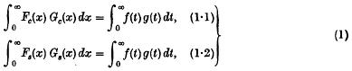
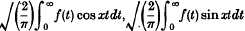
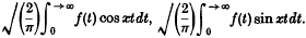
Hostname: page-component-76fb5796d-dfsvx Total loading time: 0 Render date: 2024-04-29T08:31:45.140Z Has data issue: false hasContentIssue false

The Parseval formulae for monotonic functions. I

Published online by Cambridge University Press:  24 October 2008

Sheila M. Edmonds
Affiliation:
Newnham CollegeCambridge

Extract

The Parseval formulae for Fourier cosine and sine transforms,

are of course most widely known in connexion with the classical theorems of Plancherel on functions of the class L2 (whose transforms are defined by mean convergence), and with their generalizations. We cannot expect to obtain anything as elegant as the ‘L2’ results when we consider (1) for functions of other kinds. Nevertheless, since the most obvious way of defining Fourier transforms is by means of Lebesgue or Cauchy integrals, we naturally wish to know how far the formulae (1) hold good for transforms obtained in this way. The two most familiar classes of functions having such transforms are:

(i) functions f(t) integrable in the Lebesgue sense in (0, ∞), whose transforms Fe(x) and Fs(x) are defined by the Lebesgue integrals respectively; and

(ii) functions f(t) which decrease in (0, ∞), tend to zero as t → ∞, and are integrable over any finite interval (0, T); in this case the transforms are defined by the Cauchy integrals .

Type
Research Article
Copyright
Copyright © Cambridge Philosophical Society 1947

Access options

Get access to the full version of this content by using one of the access options below. (Log in options will check for institutional or personal access. Content may require purchase if you do not have access.)

References

See, for instance, Titchmarsh, , Introduction to the Theory of Fourier Integrals (Oxford, 1937), Chapter II. This work will be referred to in future as ‘Titchmarsh’.Google Scholar

On the Parseval formulae for Fourier transforms’, Proc. Cambridge Phil. Soc. 38 (1942), 119. This paper will be referred to in the sequel as P.F. The theorem in question, here called Theorem 1, is Theorem IV of P.F. It will be convenient in future to use Arabic numerals for theorems proved in the present sequence of papers or in P.F., and Roman ones for well-known results quoted for purposes of reference; accordingly, any results from P.F. which are required here will be quoted in full and renumbered.CrossRefGoogle Scholar

We use ‘(1)’ as an abbreviation for ‘(1·1) or (1·2)’.

§ An example is given in P.F. to show that, when f and g belong to L(0, ∞) and g is monotonic, the right-hand side of (1) may exist without the left-hand side doing so. It can also be shown that if f is monotonic and Gs, belongs to L(0, ∞), the left-hand side of (1) can exist without the right-hand side doing so.

Titchmarsh, pp. 169, 170.

These properties are possessed by any convex function which is bounded in some interval (a condition which is certainly satisfied by a monotone function), or indeed by any convex measurable function. See Hardy, , Littlewood, and Pólya, , Inequalities (Cambridge, 1934), pp. 91–6, for all except the last of them.Google Scholar

An alternative version of the proof that f(T, t) increases with T may be obtained by observing that

Titchmarsh, p. 57.

Titchmarsh, , The Theory of Functions (Oxford, 1932), p. 346.Google Scholar

§ Titchmarsh, p. 54.

It was for this reason that we avoided the use of Theorem 1 in justifying (2).

An example of this kind is given in my dissertation, ‘Some multiplication problems in the theory of series and transforms’; there is a copy of this in the Cambridge University Library.

We note, however, that, while the (B*) problem is a ‘natural’ one, the (C*) problem is not; for in case [B], one side of (1·1) must exist in the finite or infinite sense, but in case [C] it is not clear that either side must do so.

In the applications which we shall make, the existence of is obvious for other reasons.

The ‘integrated terms’ vanish; for tf(t)→0 as t→0 (since f(t) is a decreasing function of L(0, 1)), and f(t)→0 as t→∞.

Saks, , Theory of the Integral (2nd ed.Warsaw, 1937), p. 77.Google Scholar

The argument is precisely that of Titchmarsh, Theorem 6, for x = 0, omitting the step in which μ is made to tend to infinity.

Titchmarsh, p. 59 (Theorem 41).

Titchmarsh, p. 12.

§ See Titchmarsh, Theorem 6, for instance.

See Titchmarsh, Theorems 22 and 74, for part of (a) and for (b); we could have treated (16) as a special case of (1·2) here as well as in (d), appealing to Titchmarsh, Theorems 35, 38, 75. The right-hand side of (16) is a Lebesgue integral since the integrand is positive; the left-hand side may be taken as a Lebesgue integral in all the cases listed.

The example is given in my dissertation, cited on p. 296. We take for f(t) a step-function with rapidly lengthening stretches of invariability, and of the same order of magnitude as 1/log2t; we then make Gs(x) oscillate violently enough near the origin.

Titchmarsh, , The Theory of Functions (Oxford, 1932), p. 346.Google Scholar

The proof may be outlined as follows. We first express Gs(x) as a sum of two functions, one of which is zero outside (0, 1), and the other, zero inside this interval. Since the latter may be disposed of by a simple ‘dominated convergence’ argument, we have only to consider functions Gs, vanishing outside (0, 1). We now apply Theorem 9 to Gs(x) − Гs(x), where Гs(x) vanishes outside (0, 1), and is equal to m, the lower bound of Gs, in (0, 1). The equation (17) holds tor f(t) and Гs(x), by Theorem 6; for Fs(x) is L(0, 1) and so Fs(x) Гs(x) is L(0, ∞). The result follows.

§ This is analogous to a well-known result on Fourier series; see Hardy, and Rogosinski, , Fourier Series (Cambridge, 1944), p. 33.Google Scholar

Young, W. H., ‘The Fourier series of bounded functions’, Proc. London Math. Soc. (2), 12 (1912), 4170 (57). Young's proof is superficially different from that given above, but is based on similar ideas.Google Scholar

This proof is suggested by Hardy and Rogosinski, loc. cit.