


Introduction
For characterization of novel materials such as ceramics, metal alloys, semiconductor systems, high-Tc superconductors, and structural study on biomaterials, one needs to have high-resolution transmission electron microscopy (HRTEM) images with an interpretable resolution down to the atomic level. The application of TEM to obtain high-resolution information involves the problem of objective lens aberrations. If the electron microscope is appropriately aligned, wave aberrations are mainly caused by spherical aberration in the objective lens. The irregular phase delays occurring due to lens aberrations must be minimized to obtain high-resolution images.
Phase contrast transfer function or contrast transfer function (CTF) describes how aberrations in an electron microscope modify the image of a sample [Reference Williams and Carter1–Reference Erni5]. By considering the recorded image as a CTF-degraded object, describing the CTF allows the object to be reverse-engineered. A comprehensive understanding of the CTF is vital to analyzing HRTEM images. In working on aberration-corrected (AC) electron microscopes, automatic correction functions do not always exhibit optimal performance. Thus, analysis of the CTF is critical to achieving the best resolution using the manual control mode.
Software programs and scripts for simulation and visualization of the CTF have been developed and are available in the public domain for conventional TEM [Reference Jiang and Chiu6–Reference Mitchell8] and AC-TEM [Reference Lee9]. Two were launched nearly twenty years ago [Reference Jiang and Chiu6,Reference Sidorov7], and the script was updated in 2017 [Reference Mitchell8]. Lee et al. [Reference Lee9] recently developed the extended CTF (exCTF) simulator to perform the primary and extensive CTF calculation designed to obtain more information than earlier software. Inspired by previous software on the CTF, we developed the CTFscope as a simulation and visualization tool of the CTF with a user-friendly interface for conventional TEM and AC-TEM. The CTFscope, as one of the components in the Landyne suite [Reference Li10], can be downloaded from the website listed in the reference. The CTFscope will help researchers better understand the instrumental performance information and effects of aberration parameters for TEM image formation through CTF simulation and visualization.
Theoretical Background and Formulas
This section briefly describes the theoretical background and the formulas used in the CTFscope for calculation. The author recommends that readers refer to the original papers and related books for more detailed information [Reference Williams and Carter1–Reference Erni5,Reference Shindo and Hiraga11–Reference Frank15]. Let us consider an electron transmission wave passing through a slice of a sample,

where σ is the interaction coefficient at the microscope accelerating voltage, ϕ p(x, y) is the specimen potential projected in the direction of the incident electron beam, and Δz is the specimen thickness through which the projection is taken. Under the kinematic scattering approximation for a “weak-phase-object,” diffractogram intensity is then written as

where V(u, v) is the Fourier coefficient of ϕ p(x, y) and sin χ(u, v) is the CTF. The first and second terms of Equation (2) correspond to the transmitted and scattered beams.
The microscope characteristic transfer function can be considered as the product of four functions, namely, the objective aperture function, the CTF, the partial spatial coherence function, and the partial temporal coherence function. Considering a circular aperture with a radius R, the aperture function can be represented as

The other three functions are given in detail below.
The CTF with basic parameters [Reference Shindo and Hiraga11]. For a conventional TEM, the χ(u, v) with the basic parameters is given by

In Equation (4), Δf and C s correspond to a defocus value and a spherical aberration coefficient of the objective lens, respectively, and λ is the wavelength of the primary electrons.
The CTF including higher order aberration parameters [Reference Uhlemann and Haider12]. For an AC-TEM, the χ(u, v) is involved with a higher order of aberration factors. A complex coordinate g = (u, v) is represented with the complex scattering angle ω by

where λ is the same term in Equation (4). The function

is a real function because of the conservation of the phase-space volume. In common notation, the power series of χ in terms of ω and its complex conjugate ${\bar\omega}$ can be written as

In Equations (6) and (7), the letters used for consistency are slightly different with Equations (3) and (4) in reference [Reference Uhlemann and Haider12].
Following commonly used convention, the index of each coefficient is the order of the corresponding ray aberration and not of the wave aberration. Here, the defocus Δf and the third-order spherical aberration Cs are addressed as C1 and C3, respectively. In Equation (4), the formula with basic parameters for conventional TEM is a simplified version of the formula above. It is worth mentioning that different label systems for the aberration coefficients were adapted in the literature [Reference Uhlemann and Haider12,Reference Lentzen13].
The CTF envelope functions [Reference O'Keefe14]. The energy fluctuation of incident electrons and their convergence on the specimen deteriorate TEM resolution. Aberration due to fluctuation of the incident electron energy is called chromatic aberration, which causes a fluctuation of focus in high-resolution images. Fluctuations in both the accelerating voltage and objective lens current contribute to the amount of focus fluctuation, that is,

where C c is the chromatic aberration coefficient for the objective lens. ${\Delta V_r\over{V_r}}$ is the fractional change in voltage over the time scale of image acquisition, and V r is the corrected accelerating voltage taking into account the relativistic effect on the electron mass. ${\Delta I\over{I}}$
 is the fractional change in lens current, and ${\Delta E\over{E}}$
 is the energy spread in the electron beam as a function of the total energy. The damping effect in scattering amplitude due to chromatic aberration, the partial temporal coherence function, is given as

while the effect due to beam convergence, partial spatial coherence function, is given by

where α indicates beam convergence, defined by the semi-angle subtended by the effective source at the specimen. These two functions are considered envelope functions that limit the contribution of scattered electrons to high-resolution images.
The dumping envelope due to drift [Reference Frank15]. Only a continuous drift case is considered here. Due to a steady drift, an object moves with constant velocity v during the exposure time T.

The dumping envelope function can be derived as

Design and Features of the CTFscope
The CTFscope was developed with Java programming language. The purpose of the software is to simulate and visualize CTF graphs for various microscope specifications, which can be specified close to experimental conditions for any specific microscope. The CTFscope provides users with an instant and intuitive simulation result for different instrumental and optical parameters. The CTF 1D and 2D graphs are displayed after the calculation according to these editable parameter values. All the parameter and simulation results are displayed using a graphical user interface (GUI).
Figure 1 shows (a) the main graphical interface of the CTFscope and (b) a dialog box of basic parameters. Users may set the instrumental parameters for specific commercial or custom microscopes. These parameters can be saved to or loaded from ASCII text files. The basic parameters include high voltage, spherical aberration coefficient Cs (C3), focal spread value, and beam convergent semi-angle. The focus value can be adjusted via a slider bar, and a marker is available for measurements. The chromatic aberration coefficient Cc and related parameters for calculating the focal spread value are in a separate dialog box (Figure 2a). The position and radius of the objective aperture and parameters of continuous drift are given in Figure 2b. Astigmatism and other higher-order aberration coefficients, up to fifth order except S5 and R5, are provided in an additional dialog box (Figure 2c). Each aberration coefficient, except the real coefficient C5, is controlled via two factors: the magnitude and azimuth angle of aberration. Labels for the parameters can be switched between the two sets of commonly used label systems [Reference Uhlemann and Haider12,Reference Lentzen13].

Figure 1: (a) The main frame of the CTFscope with graphical panel and (b) dialog box for basic microscope setup and optical parameters.
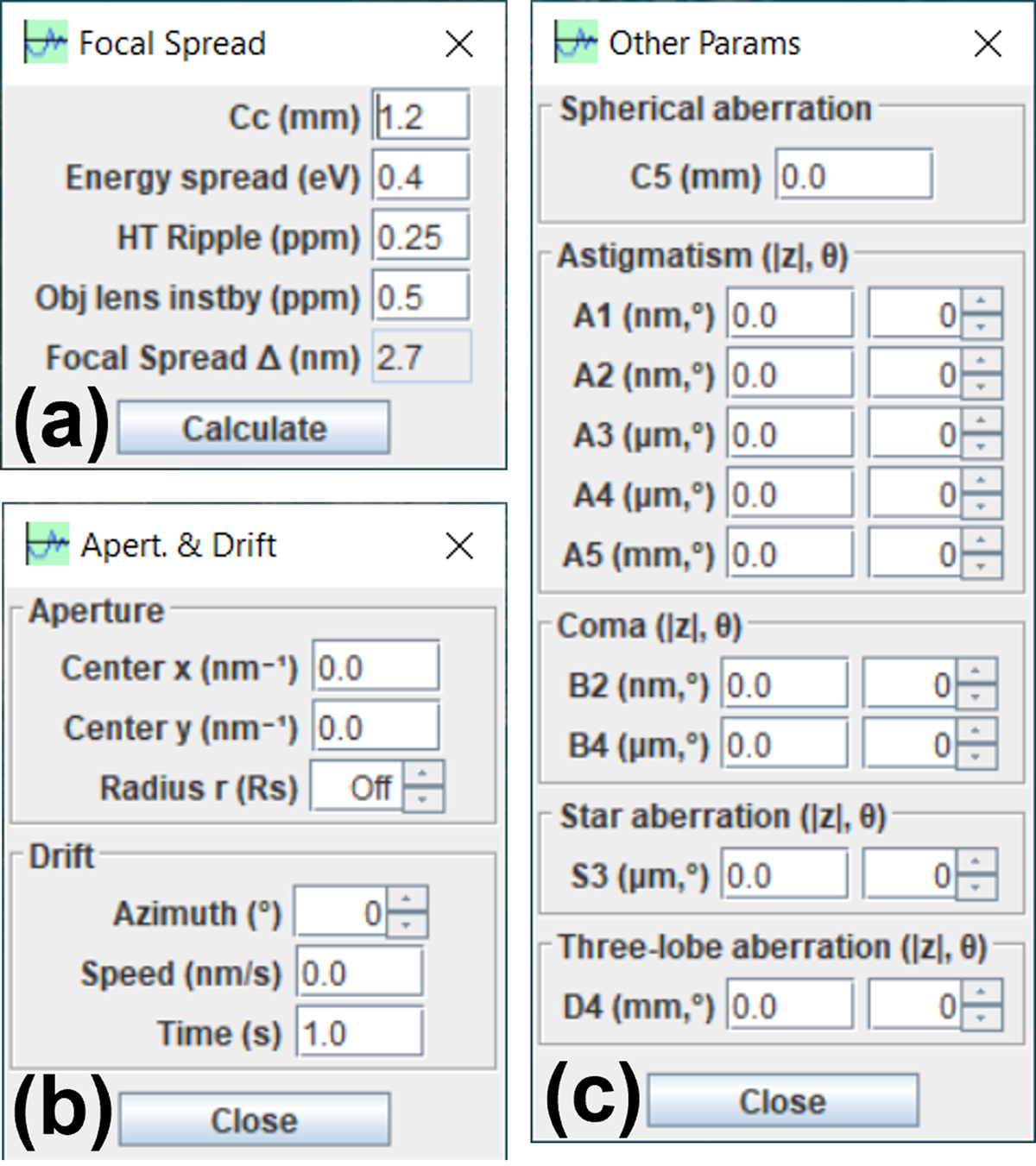
Figure 2: Dialog boxes for (a) focal spread coefficient, (b) parameters for an objective aperture and drift, and (c) astigmatism coefficients and other higher-order aberration coefficients.
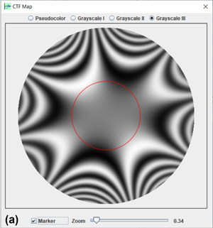
The CTF 1D and 2D graphs calculated from the default parameters are displayed in Figure 1a and Figure 3. The calculation includes envelope functions for a temporal and spatial coherence function. The 2D graph can be displayed in pseudo-color (from 0 black to -1 green and 1 blue) and three sets of grayscales: grayscale I (from 0 black to |±1| white), grayscale II (from 0 white to |±1| black), and grayscale III (from -1 black to 1 white). The circular marker is shown in Figures 3b–3d.

Figure 3: The display panel for the calculated CTF in (a) pseudo color (from 0 black to -1 green and 1 blue), (b) a grayscale I (from 0 black to |±1| white), (c) a grayscale II (from 0 white to |±1| black), and (d) a grayscale III (from -1 black to 1 white). A circular marker is in (b–d).
Calculated CTF 1D and 2D graphs can be saved as image files in various formats including TIFF, JPEG, PNG, and GIF. Furthermore, previously calculated results or experimental diffractograms may be loaded in an additional image frame for comparison with the current CTF 2D graph. For tutorial purposes, the point spread functions (PSFs) are provided as the Fourier transform of the CTF and the processed |CTF| as shown in Figure 4; an image can be loaded for processing using the two types of PSFs in 2D mode. The example images are shown in Figure 5. The PSF in Figure 4b is sharper than the one in Figure 4a, and the image in Figure 5c is sharper than the one in Figure 5b. When the CTF parameters are retrieved from the HRTEM image of an amorphous area in a TEM sample, experimental HRTEM images of crystals can be enhanced using the same method when combined with crystallographic processing. This strategy for image processing is implemented in the Simpa software in the Landyne suite [Reference Sidorov7].

Figure 4: Point spread functions as the Fourier transform of (a) the CTF and (b) |CTF|.

Figure 5: (a) An original image before processing, (b) the processed image using CTF, and (c) the processed image using |CTF|.
Let us now consider the effect of continuous drift as one of the dumping envelopes. Figure 6 shows two CTF 2D graphs with a continuous drift with parameters (a) v = 0.2 nm/s, T = 1 s, and azimuth = 0°; and (b) v = 0.2 nm/s, T = 1 s, and azimuth = 90°. Similar diffractograms of an amorphous area can be seen in TEM experiments when the sample drifts. The drift effect on an image can also be simulated by applying the CTF on the load image (not shown).

Figure 6: Two CTF 2D graphs with the continuous drift dumping effect. (a) v = 0.2 nm/s, T = 1 s, and azimuth = 0°; and (b) v = 0.2 nm/s, T = 1 s, and azimuth = 90°.
The effect of the objective aperture on an image is shown in Figure 7. When a small aperture is used (for example, a radius of half of the Scherzer resolution), the image in Figure 7a is blurred. When an aperture at the radius of Scherzer resolution is used, the image (Figure 7b) is comparable to the one in Figure 5c.

Figure 7: The processed image using a CTF with an aperture with (a) the radius as half of the Scherzer resolution and (b) the radius at Scherzer resolution.
Use of the CTFscope and Application Examples
Use of the CTFscope is straightforward. As shown in Figure 1b and Figure 2, the parameters are divided into four dialog boxes: (i) primary parameters for CTF calculation, (ii) the complementary parameters to the first dialog box, (iii) the parameters to describe an objective aperture and drift effects, and (iv) higher order aberration coefficients for an AC-TEM. The CTF, PSF-I, and PSF-II curves are automatically renewed when the parameters are updated. Dumping envelope curves can be displayed as an option. The aperture and the drift effect can also be treated as dumping envelopes. The CTF 1D and 2D graphs can be zoomed in and out separately. A marker is available for the measurement of the CTF curve. The marker can be applied on the 2D graph when the same zoom value is used on the CTF 1D and 2D graphs. An image can be loaded for comparison or as a sample image to make CTF and |CTF| transformations. All parameters can be saved to a file and reloaded. As a built-in function, Scherzer focus can be calculated and applied directly to the focus slider. The CTF 1D and 2D graphs can be saved to a file in various formats, that is, TIFF, JPEG, PNG, and GIF. Examples in the previous section were calculated using the default values. These examples can be viewed as a brief guideline for using the CTFscope. Two examples are given here to evaluate the CTFscope, in which the calculated images are compared to the figures in the published papers [Reference Lee9,Reference Uhlemann and Haider12].
The first example is a comparison of 2D graphs calculated using the CTFscope with the experimental diffractograms in Figure 1 of reference [Reference Uhlemann and Haider12], which were taken from a standard 200 kV Philips CM200ST microscope with Cs =1290 μm. Figure 8 shows CFT 2D graphs calculated using the CTFscope with the same parameters as those in Figure 1 of [Reference Uhlemann and Haider12]: (a) C1 = -633 nm, A1 = 0 nm; (b) C1 = 0 nm, A1 = 308 nm / -144°; (c) C1 = 0 nm, A1 = 85 nm / -88°; (d) C1 = -404 nm, A1 = 400 nm / -53°. The calculated CTF 2D graph matches well with the experimental diffractograms except for the central region, which is dark in the calculated graphs while bright in the diffractograms since the incident electron beam was included.

Figure 8: The 2D graphs calculated using the same parameters in Figure 1 of reference [Reference Uhlemann and Haider12].
The second example is a comparison of the results calculated using the CTFscope with other software, for example, exCTF. Figure 4 of reference [Reference Lee9] was calculated based on experimental data obtained from an AC-TEM device and compared to a calculated graph from the commercial GUI program (CETCOR, CEOS). Figure 9a shows a CTF 2D graph calculated using the CTFscope (Figure 9b–9d) using the same aberration parameters in Figure 4 of reference [Reference Lee9]. The grayscale in the CTF 2D graphs should be pointed out here. While most CTF 2D graphs use grayscale I (0 = black; both 1 and -1 = white), Figure 9a and the CTF graphs by exCTF use grayscale III (-1 = black and 1 = white). The two examples confirm that the CTFscope can provide accurate calculation and visualization results for various TEM devices.

Figure 9: (a) The CTF 2D graph without an aperture and drift, calculated using the CTFscope with (b–d), the same parameters as those in Figure 4 of reference [Reference Lee9].
Summary
The CTFscope is an interactive simulation and visualization tool for CTF graphs considering up to fifth-order aberration coefficients with temporal and spatial dumping envelopes. It also includes the envelope effects of an objective aperture and drift on the CTF, together with image transformation based on the CTF and |CTF| for tutorials. The two examples show that the CTF 2D graphs calculated using the CTFscope are congruous with the experimental results and the calculated result from published CTF software (exCTF), demonstrating that the CTFscope can effectively simulate the performance of electron microscopes and extract instrumental performance information regarding the actual resolution of AC-TEM. The CTFscope is expected to be helpful as a research tool for electron microscopy laboratories and a teaching tool for electron microscopy courses.


