Introduction
Atomic force microscopy (AFM) has been widely used in both industry and academia for imaging the surface topography of a material with nanoscale resolution. However, often little other information is obtained. Contact resonance AFM (CR-AFM) is a technique that can provide information about the viscoelastic properties of a material in contact with an AFM probe by measuring the contact stiffness between the probe and sample. In CR-AFM, an AFM cantilever is oscillated, and the amplitude and frequency of the resonance modes of the cantilever are monitored [Reference Yuya, Hurley and Turner1]. When a probe or sample is oscillated, the tip sample interaction can be approximated as an ideal spring-dashpot system using the Voigt-Kelvin model [Reference Turner, Hirsekorn, Rabe and Arnold2] shown in Figure 1. Contact resonance frequencies of the AFM cantilever will shift depending on the contact stiffness, k, between the tip and sample. The damping effect on the system comes from dissipative tip sample forces such as viscosity and adhesion. Damping, η, is observed in a CR-AFM system by monitoring the amplitude and Q factor of the resonant modes of the cantilever. This contact stiffness and damping information can then be used to obtain information about the viscoelastic properties of the material when fit to an applicable model.

Figure 1: (a) Schematic representation of contact frequency detection. The AFM laser monitors the deflection of the cantilever, and after signal processing, the frequency of oscillation of the AFM cantilever is obtained. (b) Schematic representation of the Voigt-Kelvin model for contact resonance, where k is the contact stiffness of the tip sample interaction, influenced by the stiffness of the sample surface, and η is the damping coefficient, influenced by the adhesion and viscosity.
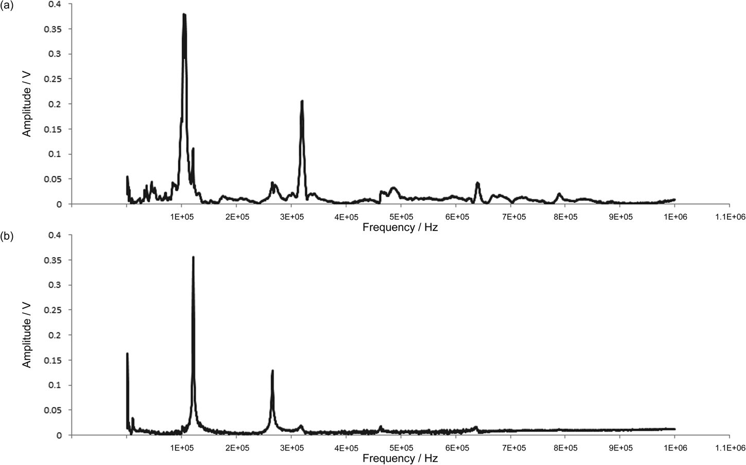
In CR-AFM there are several methods for generating an oscillation in a cantilever, including ultrasonic AFM [Reference Yamanaka, Maruyama, Tsuji and Nakamoto3] and atomic force acoustic microscopy [Reference Rabe, Kopycinska, Hirsekorn, Saldana, Schneider and Arnold4]. In these methods the oscillation is driven by a piezo, either behind the cantilever or under the sample; however, when oscillations are driven by a piezo there are often many spurious resonances from the piezo itself. This article describes Lorentz contact resonance AFM (LCR-AFM), a new technique that allows monitoring of contact resonances, between a ThermaLever™ AFM probe and a sample, without the spurious resonances associated with piezo-driven systems (see Figure 2).
Figure 2: (a) CR-AFM spectrum acquired using a piezo-driven ThermaLever AFM cantilever (many parasitic resonances). (b) CR-AFM spectrum acquired using a LCR-driven ThermaLever AFM cantilever.
Lorentz Contact Resonance Mode
Lorentz contact resonance mode is an AFM imaging mode, available on all Anasys Instruments AFM systems, that allows the user to image the surface of a sample with image contrast derived from the relative stiffness of each component within the sample. Furthermore, the contact resonance modes of the AFM cantilever can be monitored using Analysis Studio™ software. As the name suggests, the drive mechanism in LCR-AFM is based on an oscillating Lorentzian force [Reference Lee, Prater and King5]. When a magnetic field interacts perpendicularly with a current in a wire, a force is generated that is perpendicular to both the current and magnetic field. If an alternating current is applied, then the force occurs in two directions, generating an oscillation in the cantilever (Figure 3).
Figure 3: A schematic representation of how the LCR drive works. The perpendicular interaction of the magnetic field and the alternating current flowing through the cantilever induces an oscillation in the cantilever due to the Lorentzian forces that are generated.
Using the sweep control panel in the Analysis Studio software, the user can vary the frequency of the A/C drive signal sent down the cantilever over a wide range, 1 kHz– 4 MHz (shown in Figure 4). When the frequency is swept, the resulting nanomechanical spectrum indicates the frequency and amplitude of each of the contact resonance modes of the ThermaLever cantilever. The large frequency sweep range allows for probing a wide range of sample stiffness with a single cantilever. This technique is made possible by the use of ThermaLever cantilevers, which are batch-fabricated AFM cantilevers composed of doped silicon. The two-legged design of these cantilevers provides a path for flowing the alternating current required for the generation of the Lorentzian force. Furthermore, these ThermaLever cantilevers have a resistive heater element integrated into the end of the cantilever, allowing controlled heating of the probe when direct current is supplied, to a maximum temperature of ~400°C.
Figure 4: The sweep control panel in the Analysis Studio™ software, where the user can control the start and end frequency as well as the sweep rate of the AC frequency through the ThermaLever cantilever.
Results
Polymer blend. Today's polymer blends are more complex than ever, leading to challenges in characterizing the distribution of components in the blend. Figure 5 shows a typical AFM height image of a three-component polymer blend. The only information obtained from such topographical images is of the overall morphology of the sample surface.
Figure 5: AFM topographical image of a three-component polymer blend.
The distribution of domains within a polymer blend greatly affects the overall performance of the polymer. Although conventional AFM can provide a topographical image of a polymer blend, the blend distribution cannot be determined. Although phase imaging can sometimes differentiate between different materials, the contrast derived from phase imaging is based on a number of factors, including friction, viscosity, and adhesion. The LCR-AFM mode provides contrast based on the contact stiffness between the tip and sample, allowing for the differentiation of materials with similar stiffness that may not be clearly observed by phase imaging.
Figure 6 shows the nanomechanical spectra for each component of the three-component polymer blend, acquired by first placing the probe on one component, sweeping the drive frequency to the probe, and monitoring the cantilever contact resonances. As shown in the spectra of Figure 6, the contact resonant frequency of the elastomer is shifted farthest left, indicating it is the softest material. Although the polycarbonate and polypropylene do not display large shifts in contact frequency, because they have similar Young's moduli, they can still be differentiated by their contact resonance amplitudes, that is, different dissipation properties.
Figure 6: Nanomechanical spectra of elastomer (green), polycarbonate (red), and polypropylene (blue). Each peak in the spectrum represents a contact resonance mode of the cantilever. The frequency and amplitude of each peak indicate the relative stiffness of each area probed, with softer materials appearing at lower frequencies.
Once these different components have been identified by nanomechanical spectroscopy, it is then possible to image each component individually. This is achieved by tuning the drive signal to the ThermaLever cantilever to an observed contact resonance frequency for a material and collecting an LCR-AFM amplitude image. Figure 7 shows images of the individual components in this polymer blend along with an RGB overlay image, displaying the individual domains of each component in a single image.
Figure 7: Polymer blend components distinguished. LCR-AFM maps distinguishing (a) polypropylene, (b) polycarbonate, and (c) elastomer. These individual LCR-AFM images were produced by tuning the AC frequency through the probe to the contact resonance frequency of each individual component, as seen in the nanomechanical spectra (Figure 6). (d) RGB overlay image of the three individual component images, highlighting the distribution of each component. Image width = 10 μm.
One additional benefit of LCR imaging is that it allows for enhanced positioning of the ThermaLever for subsequent nanoTA measurements. Figure 8a shows an LCR-AFM image with three measurement locations on polypropylene and three on polycarbonate. The thermal analyses of Figure 8b show a distinct thermal transition for each polymer component.
Figure 8: (a) LCR-AFM image of three-component polymer blend. (b) nanoTA data for two of the components (green: polypropylene and blue: polycarbonate), indicating the onset of glass transition or melt temperature for each component within the polymer blend with nanoscale spatial resolution (polypropylene: 129°C and polycarbonate: 153°C).
Multilayer film. Multilayer films are key materials in the packaging industry. These multilayer films may have many layers of different materials with vastly different mechanical and thermal properties to provide optimum performance. Quality control and characterization of these manufactured multilayer films is important; interior layers of these films may be damaged or altered during the film forming process.
The LCR-AFM mode provides the ability to characterize the relative mechanical properties of all the layers of a preformed film along with corresponding thermal properties (Tg or Tm). Sample preparation for this example is a simple process of embedding the multilayer film in epoxy and exposing a smooth cross-sectioned surface via microtoming. Figure 9a shows an AFM topographic image of an 8-layer film, where color-coded markings on the image indicate the positioning of the ThermaLever probe for subsequent nanomechanical spectroscopy measurements. Figure 9b shows nanomechanical spectra of each layer indicating the relative stiffness. This allows easy monitoring of layer ordering, based on the expected relative stiffnesses. Nanomechanical spectroscopy may also indicate unwanted changes in the mechanical properties of each layer during the film forming process.
Figure 9: (a) AFM topography image of the sectioned multilayer film. (b) Nanomechanical spectra for each individual layer within the multilayer film obtained by sweeping the frequency of the AC voltage flowing down the cantilever and recording the contact resonance frequencies for each component. The lower the contact frequency, the softer the layer being probed. Image width = 80 μm.
Figures 10 and 11 show thermal analysis measurements on the same material. Figure 10 shows that the boundary between layers is clearly defined, allowing accurate measurements of the thickness of each layer. The thickness of each layer can play an important role in the overall performance of the film. Currently these multilayer films are peeled apart and examined using bulk thermal analysis techniques such as differential scanning calorimetry (DSC), a labor- and time-intensive process. As previously mentioned, ThermaLever probes have a resistive heating element integrated into the end of the cantilever, allowing for controlled heating of the probe. The tool allows for the determination of thermal transitions (Tg or Tm) by monitoring the deflection of the AFM cantilever. The sample will expand during heating, causing a change in deflection of the cantilever. The probe will then penetrate into the sample when a transition occurs, resulting in a change in cantilever deflection. Figure 11 shows nanoTA results that identify the thermal transitions for each layer in the film without the need for laborious sample preparation.
Figure 10: Measurements on a multi-layer polymer film. LCR-AFM image highlighting layer boundaries (markers indicate positions for subsequent nanoTA measurements).
Figure 11: Local thermal analysis by nanoTA indicates the thermal transitions (glass or melt) for each layer within the multilayer film (color indicates position of measurement in 9a). The deflection of the AFM probe is monitored, with the penetration of the probe into the sample indicating the onset of the thermal transition.
Carbon nanomaterials in a polymer matrix. The dispersion of a component in a polymer matrix plays a key role in the performance of a composite. When working with nanocomposites, one of the most important factors influencing the performance of the composite is the mixing conditions. When poor mixing is used, the resulting blend may have multiple defect sites that could lead to a catastrophic failure of the product. The most commonly used techniques for the characterization of dispersion are a combination of X-ray diffraction (XRD) with scanning electron microscopy (SEM) or transmission electron microscopy (TEM). Both of these imaging techniques have significant drawbacks. With TEM, the sample must be very thin to allow for the transmission of the electron beam; whereas, SEM analysis usually requires the sample to be conductive, which is generally not the case with most polymer nanocomposites. In sample preparation for SEM analysis of nanocomposites, cryofracturing is a commonly used method; however, the nanocomposite is most likely to fracture in weak areas where the dispersion may be poor. This may lead to an inaccurate characterization of the dispersion.
The LCR-AFM mode allows the user to probe the distribution of components in a polymer matrix by imaging each component individually, with image contrast usually caused by the differing viscoelastic properties of the components. In the example shown in Figure 12, the dispersion of a carbon nanomaterial in a polymer matrix was monitored. Various mixing conditions were applied, and the resulting composites (1, 2, and 3) were analyzed using the afm+™ system (Anasys Instruments). Figure 12 shows that the mixing conditions used in the preperation of composite 1 resulted in the aggregation of the carbon nanomaterial. The nanomechanical spectra indicate the aggregated carbon domains are significantly stiffer than the surroundimg matrix.
Figure 12: Dispersion of carbon nanomaterials in a polymer matrix. (a) Nanomechanical spectra of aggregated carbon material (blue) and surrounding polymer matrix (green) with spectra indicating the relative stiffness of each domain. (b) Corresponding LCR-AFM amplitude image for composite 1. Image width = 80 μm.
Figure 13 shows LCR-AFM imaging results for two additional sets of nanocarbon composites that were prepared with different mixing conditions. As can be seen from Figure 13b, composite 2 contains regions of good dispersion, some aggregation, and no disperion at all. The detection of regions of no carbon dispersion is important and may not have been discovered using the cryofracture SEM technique because the components would most likely fracture in this region. The LCR-AFM image of composite 3, Figure 13d, shows good dispersion of the carbon nanomaterial within the matrix.
Figure 13: Comparison of nanocarbon composites prepared under different mixing conditions. (a) AFM topography image of composite 2, with round regions being large aggregates of nanomaterial. (b) LCR-AFM image of composite 2. (c) AFM topography image of composite 3. (d) LCR-AFM image of composite 3, with the fine granularity indicating good dispersion. (Banding in the images is caused by the microtome blade.) Image width = 20 μm.
Conclusions
Lorentz contact resonance AFM provides an enhanced ability to characterize various types of polymeric samples when compared to conventional AFM. Phase imaging in AFM is limited by a number of factors that influence the contrast achieved during phase imaging, including adhesion and viscosity. The ability of LCR-AFM to tune the probe oscillation in an Anasys Instruments system to the contact resonance frequency for a particular component gives image contrast based only on stiffness. This is a significant advancement over phase imaging because it can differentiate materials with similar stiffness where phase imaging cannot. The combination in the nanoIR™ instrument of LCR-AFM, nanoTA, and AFM-IR provides the user with a multifunctional tool capable of characterizing a sample topographically, thermally, and chemically with high spatial resolution.
Acknowledgments
The authors would like to thank Dr. Greg Myers from Dow Chemical Company for providing a three-component polymer blend sample and Dr. Sayantan Roy at Baker Hughes Inc. for providing the nano-carbon composite materials.