


1 Introduction and statement of results
A local Borcherds product is a holomorphic function, which, like a Borcherds form has an absolutely convergent infinite product expansion and an arithmetically defined divisor, called a local Heegner divisor. Here, “local” refers to boundary components of a modular variety. Such products were first introduced by Bruinier and Freitag [Reference Bruinier and Freitag4], who studied the local divisor class groups of generic boundary components for the modular varieties of indefinite orthogonal groups
 $\text{O}(2,l)$
,
$\text{O}(2,l)$
,
 $l\geqslant 3$
. Since then, local Borcherds products have appeared in several places in the literature, for example in [Reference Bruinier, van der Geer, Harder and Zagier6], for the Hilbert modular group, and in [Reference Freitag and Salvati Manni7], where they are introduced to study a specific problem in the geometry of Siegel three folds.
$l\geqslant 3$
. Since then, local Borcherds products have appeared in several places in the literature, for example in [Reference Bruinier, van der Geer, Harder and Zagier6], for the Hilbert modular group, and in [Reference Freitag and Salvati Manni7], where they are introduced to study a specific problem in the geometry of Siegel three folds.
The aim of the present paper is to develop a theory similar to that of Bruinier and Freitag for unitary groups of signature
 $(1,n+1)$
,
$(1,n+1)$
,
 $n\geqslant 1$
.
$n\geqslant 1$
.
Let
 $\mathbf{k}=\mathbb{Q}(\sqrt{D_{\mathbf{k}}})$
be an imaginary quadratic number field with discriminant
$\mathbf{k}=\mathbb{Q}(\sqrt{D_{\mathbf{k}}})$
be an imaginary quadratic number field with discriminant
 $D_{\mathbf{k}}$
, which we consider as a subset of
$D_{\mathbf{k}}$
, which we consider as a subset of
 $\mathbb{C}$
. Denote by
$\mathbb{C}$
. Denote by
 ${\mathcal{O}}_{\mathbf{k}}$
the ring of integers in
${\mathcal{O}}_{\mathbf{k}}$
the ring of integers in
 $\mathbf{k}$
, by
$\mathbf{k}$
, by
 $\mathfrak{d}_{\mathbf{k}}^{-1}$
the inverse different ideal and by
$\mathfrak{d}_{\mathbf{k}}^{-1}$
the inverse different ideal and by
 $\unicode[STIX]{x1D6FF}_{\mathbf{k}}$
the square root of
$\unicode[STIX]{x1D6FF}_{\mathbf{k}}$
the square root of
 $D_{\mathbf{k}}$
, with the principal branch of the complex square root.
$D_{\mathbf{k}}$
, with the principal branch of the complex square root.
Let
 $V$
be an indefinite Hermitian vector space over
$V$
be an indefinite Hermitian vector space over
 $\mathbf{k}$
of signature
$\mathbf{k}$
of signature
 $(1,n+1)$
, equipped with a nondegenerate Hermitian form
$(1,n+1)$
, equipped with a nondegenerate Hermitian form
 $\langle \cdot ,\cdot \rangle$
. Let
$\langle \cdot ,\cdot \rangle$
. Let
 $L$
be a lattice in
$L$
be a lattice in
 $V$
, of full rank as an
$V$
, of full rank as an
 ${\mathcal{O}}_{\mathbf{k}}$
-module, so that
${\mathcal{O}}_{\mathbf{k}}$
-module, so that
 $L\otimes _{{\mathcal{O}}_{\mathbf{k}}}\mathbf{k}=V$
. We assume that
$L\otimes _{{\mathcal{O}}_{\mathbf{k}}}\mathbf{k}=V$
. We assume that
 $L$
is an even and integral lattice, hence
$L$
is an even and integral lattice, hence
 $\langle \unicode[STIX]{x1D706},\unicode[STIX]{x1D706}\rangle \in \mathbb{Z}$
for all
$\langle \unicode[STIX]{x1D706},\unicode[STIX]{x1D706}\rangle \in \mathbb{Z}$
for all
 $\unicode[STIX]{x1D706}\in L$
. In this introductory section only, we additionally assume that
$\unicode[STIX]{x1D706}\in L$
. In this introductory section only, we additionally assume that
 $L$
is unimodular over
$L$
is unimodular over
 $\mathbb{Z}$
, that is
$\mathbb{Z}$
, that is
 $L=L^{\prime }=\{\unicode[STIX]{x1D707}\in V;\;\langle \unicode[STIX]{x1D706},\unicode[STIX]{x1D707}\rangle \in \mathfrak{d}_{\mathbf{k}}^{-1},\forall \unicode[STIX]{x1D706}\in L\}$
.
$L=L^{\prime }=\{\unicode[STIX]{x1D707}\in V;\;\langle \unicode[STIX]{x1D706},\unicode[STIX]{x1D707}\rangle \in \mathfrak{d}_{\mathbf{k}}^{-1},\forall \unicode[STIX]{x1D706}\in L\}$
.
We denote by
 $\text{U}(V)$
the unitary group of
$\text{U}(V)$
the unitary group of
 $V$
and by
$V$
and by
 $\text{U}(L)\subset \text{U}(V)$
the isometry group of
$\text{U}(L)\subset \text{U}(V)$
the isometry group of
 $L$
. Subgroups of finite index in
$L$
. Subgroups of finite index in
 $\text{U}(L)$
are called unitary modular groups.
$\text{U}(L)$
are called unitary modular groups.
We consider
 $\text{U}(V)$
as an algebraic group defined over
$\text{U}(V)$
as an algebraic group defined over
 $\mathbb{Q}$
. Its set of real points, denoted
$\mathbb{Q}$
. Its set of real points, denoted
 $\text{U}(V)(\mathbb{R})$
, is the unitary group of the complex Hermitian space
$\text{U}(V)(\mathbb{R})$
, is the unitary group of the complex Hermitian space
 $V\otimes _{\mathbf{k}}\mathbb{C}$
. A symmetric domain for the operation of this group is given by the quotient
$V\otimes _{\mathbf{k}}\mathbb{C}$
. A symmetric domain for the operation of this group is given by the quotient
 $$\begin{eqnarray}\mathbb{D}=\text{U}(V)(\mathbb{R})/{\mathcal{K}},\end{eqnarray}$$
where
 ${\mathcal{K}}$
is a maximal compact subgroup of
${\mathcal{K}}$
is a maximal compact subgroup of
 $\text{U}(V)(\mathbb{R})$
. If
$\text{U}(V)(\mathbb{R})$
. If
 $\unicode[STIX]{x1D6E4}\subset \text{U}(L)$
is a unitary modular group, we denote by
$\unicode[STIX]{x1D6E4}\subset \text{U}(L)$
is a unitary modular group, we denote by
 $X_{\unicode[STIX]{x1D6E4}}$
the modular variety given by the quotient
$X_{\unicode[STIX]{x1D6E4}}$
the modular variety given by the quotient
 $\unicode[STIX]{x1D6E4}\backslash \mathbb{D}$
. Note that
$\unicode[STIX]{x1D6E4}\backslash \mathbb{D}$
. Note that
 $X_{\unicode[STIX]{x1D6E4}}$
is noncompact.
$X_{\unicode[STIX]{x1D6E4}}$
is noncompact.
The boundary points of
 $\mathbb{D}$
correspond one to one to the elements
$\mathbb{D}$
correspond one to one to the elements
 $I$
of the set of rational one-dimensional isotropic subspaces of
$I$
of the set of rational one-dimensional isotropic subspaces of
 $V$
, denoted
$V$
, denoted
 $\text{Iso}(V)$
. For every cusp of
$\text{Iso}(V)$
. For every cusp of
 $X_{\unicode[STIX]{x1D6E4}}$
one can thus introduce a small open neighborhood
$X_{\unicode[STIX]{x1D6E4}}$
one can thus introduce a small open neighborhood
 $U_{\unicode[STIX]{x1D716}}(I)$
. These neighborhoods are then glued to
$U_{\unicode[STIX]{x1D716}}(I)$
. These neighborhoods are then glued to
 $X_{\unicode[STIX]{x1D6E4}}$
, furnishing a compactification. We describe this procedure in Section 2.4 both for the Baily–Borel compactification, in which singularities remain at the cusps, and for a toroidal compactification, which turns
$X_{\unicode[STIX]{x1D6E4}}$
, furnishing a compactification. We describe this procedure in Section 2.4 both for the Baily–Borel compactification, in which singularities remain at the cusps, and for a toroidal compactification, which turns
 $X_{\unicode[STIX]{x1D6E4}}$
into a normal complex space without singularities at the cusps.
$X_{\unicode[STIX]{x1D6E4}}$
into a normal complex space without singularities at the cusps.
We study the Picard groups of such (suitably small) open neighborhoods
 $U_{\unicode[STIX]{x1D716}}(I)$
. Since the construction we carry out is local in nature, it suffices to examine only one fixed cusp. For this purpose, we choose a primitive isotropic lattice vector
$U_{\unicode[STIX]{x1D716}}(I)$
. Since the construction we carry out is local in nature, it suffices to examine only one fixed cusp. For this purpose, we choose a primitive isotropic lattice vector
 $\ell \in L$
. Fixing a vector
$\ell \in L$
. Fixing a vector
 $\ell ^{\prime }\in L$
with
$\ell ^{\prime }\in L$
with
 $\langle \ell ,\ell ^{\prime }\rangle \neq 0$
, denote by
$\langle \ell ,\ell ^{\prime }\rangle \neq 0$
, denote by
 $D$
the definite lattice
$D$
the definite lattice
 $L\cap \ell ^{\bot }\cap {\ell ^{\prime }}^{\bot }$
. The stabilizer
$L\cap \ell ^{\bot }\cap {\ell ^{\prime }}^{\bot }$
. The stabilizer
 $\operatorname{Stab}_{\unicode[STIX]{x1D6E4}}(\ell )$
of
$\operatorname{Stab}_{\unicode[STIX]{x1D6E4}}(\ell )$
of
 $\ell$
in
$\ell$
in
 $\unicode[STIX]{x1D6E4}$
contains a Heisenberg group, denoted
$\unicode[STIX]{x1D6E4}$
contains a Heisenberg group, denoted
 $\unicode[STIX]{x1D6E4}_{\ell }$
. This group has finite index in the stabilizer. Its elements can be written as pairs
$\unicode[STIX]{x1D6E4}_{\ell }$
. This group has finite index in the stabilizer. Its elements can be written as pairs
 $[h,t]$
, with
$[h,t]$
, with
 $h$
a rational number and
$h$
a rational number and
 $t$
a lattice vector. The set of all such
$t$
a lattice vector. The set of all such
 $t$
’s constitutes a sublattice
$t$
’s constitutes a sublattice
 $D_{\ell ,\unicode[STIX]{x1D6E4}}\subseteq D$
.
$D_{\ell ,\unicode[STIX]{x1D6E4}}\subseteq D$
.
Following [Reference Bruinier and Freitag4], we define the Picard group
 $\text{Pic}(X_{\unicode[STIX]{x1D6E4}},\ell )$
as the direct limit
$\text{Pic}(X_{\unicode[STIX]{x1D6E4}},\ell )$
as the direct limit
 $\varinjlim \text{Pic}(U_{\unicode[STIX]{x1D716}}^{\text{reg}}(\ell ))$
, where
$\varinjlim \text{Pic}(U_{\unicode[STIX]{x1D716}}^{\text{reg}}(\ell ))$
, where
 $U_{\unicode[STIX]{x1D716}}^{\text{reg}}(\ell )$
is the regular locus of
$U_{\unicode[STIX]{x1D716}}^{\text{reg}}(\ell )$
is the regular locus of
 $U_{\unicode[STIX]{x1D716}}(\ell )$
in the Baily–Borel compactification.
$U_{\unicode[STIX]{x1D716}}(\ell )$
in the Baily–Borel compactification.
Up to torsion, this local Picard group can also be described by the direct limit
 $\varinjlim \text{Pic}(\unicode[STIX]{x1D6E4}_{\ell }\backslash U_{\unicode[STIX]{x1D716}}(\ell ))$
, see p. 152 for details. Thus, if we only want to describe the position of certain special divisors in
$\varinjlim \text{Pic}(\unicode[STIX]{x1D6E4}_{\ell }\backslash U_{\unicode[STIX]{x1D716}}(\ell ))$
, see p. 152 for details. Thus, if we only want to describe the position of certain special divisors in
 $\text{Pic}(X_{\unicode[STIX]{x1D6E4}},\ell )$
up to torsion, we can work in
$\text{Pic}(X_{\unicode[STIX]{x1D6E4}},\ell )$
up to torsion, we can work in
 $\text{Pic}(\unicode[STIX]{x1D6E4}_{\ell }\backslash U_{\unicode[STIX]{x1D716}}(\ell ))$
, with a sufficiently small
$\text{Pic}(\unicode[STIX]{x1D6E4}_{\ell }\backslash U_{\unicode[STIX]{x1D716}}(\ell ))$
, with a sufficiently small
 $\unicode[STIX]{x1D716}>0$
.
$\unicode[STIX]{x1D716}>0$
.
For a lattice vector
 $\unicode[STIX]{x1D706}\in L$
of negative norm, that is
$\unicode[STIX]{x1D706}\in L$
of negative norm, that is
 $\langle \unicode[STIX]{x1D706},\unicode[STIX]{x1D706}\rangle \in \mathbb{Z}_{{<}0}$
, a primitive Heegner divisor
$\langle \unicode[STIX]{x1D706},\unicode[STIX]{x1D706}\rangle \in \mathbb{Z}_{{<}0}$
, a primitive Heegner divisor
 $\mathbf{H}(\unicode[STIX]{x1D706})$
is defined by the orthogonal complement
$\mathbf{H}(\unicode[STIX]{x1D706})$
is defined by the orthogonal complement
 $\unicode[STIX]{x1D706}^{\bot }$
with respect to
$\unicode[STIX]{x1D706}^{\bot }$
with respect to
 $\langle \cdot ,\cdot \rangle$
of
$\langle \cdot ,\cdot \rangle$
of
 $\unicode[STIX]{x1D706}$
in
$\unicode[STIX]{x1D706}$
in
 $\mathbb{D}$
. If
$\mathbb{D}$
. If
 $\ell$
lies in
$\ell$
lies in
 $\unicode[STIX]{x1D706}^{\bot }$
, we attach a local Heegner divisor to
$\unicode[STIX]{x1D706}^{\bot }$
, we attach a local Heegner divisor to
 $\unicode[STIX]{x1D706}$
by setting
$\unicode[STIX]{x1D706}$
by setting
 $\mathbf{H}_{\infty }(\unicode[STIX]{x1D706}):=\sum _{\unicode[STIX]{x1D6FC}\in \mathfrak{d}_{\mathbf{k}}^{-1}}\mathbf{H}(\unicode[STIX]{x1D706}+\unicode[STIX]{x1D6FC}\ell )$
.
$\mathbf{H}_{\infty }(\unicode[STIX]{x1D706}):=\sum _{\unicode[STIX]{x1D6FC}\in \mathfrak{d}_{\mathbf{k}}^{-1}}\mathbf{H}(\unicode[STIX]{x1D706}+\unicode[STIX]{x1D6FC}\ell )$
.
A Heegner divisor of
 $\mathbb{D}$
is a
$\mathbb{D}$
is a
 $\unicode[STIX]{x1D6E4}$
-invariant finite linear combination of primitive Heegner divisors and the pre-image under the canonical projection of a divisor on
$\unicode[STIX]{x1D6E4}$
-invariant finite linear combination of primitive Heegner divisors and the pre-image under the canonical projection of a divisor on
 $X_{\unicode[STIX]{x1D6E4}}$
. By a local Heegner divisor, we mean a finite linear combination of local Heegner divisors of the form
$X_{\unicode[STIX]{x1D6E4}}$
. By a local Heegner divisor, we mean a finite linear combination of local Heegner divisors of the form
 $\mathbf{H}_{\infty }(\unicode[STIX]{x1D706})$
, which corresponds to the pre-image of an element of the divisor group
$\mathbf{H}_{\infty }(\unicode[STIX]{x1D706})$
, which corresponds to the pre-image of an element of the divisor group
 $\text{Div}(\unicode[STIX]{x1D6E4}_{\ell }\backslash U_{\unicode[STIX]{x1D716}}(\ell ))$
, see Section 4.1 for details.
$\text{Div}(\unicode[STIX]{x1D6E4}_{\ell }\backslash U_{\unicode[STIX]{x1D716}}(\ell ))$
, see Section 4.1 for details.
We want to describe the position of local Heegner divisors in the local Picard group
 $\text{Pic}(X_{\unicode[STIX]{x1D6E4}},\ell )$
(up to torsion) through their position in
$\text{Pic}(X_{\unicode[STIX]{x1D6E4}},\ell )$
(up to torsion) through their position in
 $\text{Pic}(\unicode[STIX]{x1D6E4}_{\ell }\backslash U_{\unicode[STIX]{x1D716}}(\ell ))$
. This is where local Borcherds products come into play. For a negative-norm lattice vector
$\text{Pic}(\unicode[STIX]{x1D6E4}_{\ell }\backslash U_{\unicode[STIX]{x1D716}}(\ell ))$
. This is where local Borcherds products come into play. For a negative-norm lattice vector
 $\unicode[STIX]{x1D706}$
we define the local Borcherds product
$\unicode[STIX]{x1D706}$
we define the local Borcherds product
 $\unicode[STIX]{x1D6F9}_{\unicode[STIX]{x1D706}}(z)$
as follows (see Section 4.2):
$\unicode[STIX]{x1D6F9}_{\unicode[STIX]{x1D706}}(z)$
as follows (see Section 4.2):
 $$\begin{eqnarray}\unicode[STIX]{x1D6F9}_{\unicode[STIX]{x1D706}}(z):=\mathop{\prod }_{\unicode[STIX]{x1D6FC}\in \mathfrak{d}_{\mathbf{k}}^{-1}}(1-e(\unicode[STIX]{x1D70E}(\unicode[STIX]{x1D6FC})\langle z,\unicode[STIX]{x1D706}-\unicode[STIX]{x1D6FC}\ell \rangle )).\end{eqnarray}$$
Here,
 $\unicode[STIX]{x1D706}-\unicode[STIX]{x1D6FC}\ell$
runs over finitely many orbits under the operation of
$\unicode[STIX]{x1D706}-\unicode[STIX]{x1D6FC}\ell$
runs over finitely many orbits under the operation of
 $\unicode[STIX]{x1D6E4}_{\ell }$
, and
$\unicode[STIX]{x1D6E4}_{\ell }$
, and
 $\unicode[STIX]{x1D70E}(\unicode[STIX]{x1D707})$
is a sign introduced to assure absolute convergence. The product has divisor
$\unicode[STIX]{x1D70E}(\unicode[STIX]{x1D707})$
is a sign introduced to assure absolute convergence. The product has divisor
 $\mathbf{H}_{\infty }(\unicode[STIX]{x1D706})$
. However, because of the sign
$\mathbf{H}_{\infty }(\unicode[STIX]{x1D706})$
. However, because of the sign
 $\unicode[STIX]{x1D70E}(\unicode[STIX]{x1D6FC})$
, it is not invariant under
$\unicode[STIX]{x1D70E}(\unicode[STIX]{x1D6FC})$
, it is not invariant under
 $\unicode[STIX]{x1D6E4}_{\ell }$
. Instead, there is a nontrivial automorphy factor.
$\unicode[STIX]{x1D6E4}_{\ell }$
. Instead, there is a nontrivial automorphy factor.
This is actually a desirable situation: by calculating the automorphy factor, we are able to determine the Chern class of
 $\mathbf{H}_{\infty }(\unicode[STIX]{x1D706})$
in the cohomology group
$\mathbf{H}_{\infty }(\unicode[STIX]{x1D706})$
in the cohomology group
 $\text{H}^{2}(\unicode[STIX]{x1D6E4}_{\ell },\mathbb{Z})$
(see Sections 4.2 and 4.3). It turns out to be given by the image
$\text{H}^{2}(\unicode[STIX]{x1D6E4}_{\ell },\mathbb{Z})$
(see Sections 4.2 and 4.3). It turns out to be given by the image
 $[c_{\unicode[STIX]{x1D706}}]$
of a bilinear form in the cohomology:
$[c_{\unicode[STIX]{x1D706}}]$
of a bilinear form in the cohomology:
 $$\begin{eqnarray}\begin{array}{@{}c@{}}\displaystyle c_{\unicode[STIX]{x1D706}}([h,t],[h^{\prime },t^{\prime }])=-\Im [|\unicode[STIX]{x1D6FF}_{\mathbf{k}}|F_{\unicode[STIX]{x1D706}}(t,t^{\prime })]\quad (\text{for }[h,t],[h^{\prime },t^{\prime }]\in \unicode[STIX]{x1D6E4}_{\ell }),\\ \displaystyle \text{where }F_{\unicode[STIX]{x1D706}}(x,y):=\langle x,\unicode[STIX]{x1D706}\rangle \langle y,\unicode[STIX]{x1D706}\rangle +\langle \unicode[STIX]{x1D706},x\rangle \langle y,\unicode[STIX]{x1D706}\rangle \quad (x,y\in D\otimes _{{\mathcal{O}}_{\mathbf{k}}}\mathbb{C}).\end{array}\end{eqnarray}$$
Through this, we know the Chern class of every local Heegner divisor as a finite linear combination, and can thus describe its position in the cohomology.
For this we use results prepared in Section 3, from calculations in the group cohomology for
 $\unicode[STIX]{x1D6E4}_{\ell }$
, concerning the properties of cocycles in
$\unicode[STIX]{x1D6E4}_{\ell }$
, concerning the properties of cocycles in
 $\text{H}^{2}(\unicode[STIX]{x1D6E4}_{\ell },\mathbb{Z})$
. We obtain an equivalent condition for the Chern class of a linear combination of Heegner divisors to be a torsion element, in Lemma 4.1. From the proof, we also obtain a further, necessary condition, see Corollary 4.1. Finally, our main result, Theorem 4.1, describes exactly when Heegner divisors are torsion elements in the Picard group
$\text{H}^{2}(\unicode[STIX]{x1D6E4}_{\ell },\mathbb{Z})$
. We obtain an equivalent condition for the Chern class of a linear combination of Heegner divisors to be a torsion element, in Lemma 4.1. From the proof, we also obtain a further, necessary condition, see Corollary 4.1. Finally, our main result, Theorem 4.1, describes exactly when Heegner divisors are torsion elements in the Picard group
 $\text{Pic}(\unicode[STIX]{x1D6E4}_{\ell }\backslash U_{\unicode[STIX]{x1D716}}(\ell ))$
. For a unimodular lattice
$\text{Pic}(\unicode[STIX]{x1D6E4}_{\ell }\backslash U_{\unicode[STIX]{x1D716}}(\ell ))$
. For a unimodular lattice
 $L$
, the theorem can be formulated as follows, for the general version, see Theorem 4.1 on p. 161:
$L$
, the theorem can be formulated as follows, for the general version, see Theorem 4.1 on p. 161:
Theorem 1.1. A finite linear combination of local Heegner divisors of the form
 $$\begin{eqnarray}\mathbf{H}=\frac{1}{2}\mathop{\sum }_{\substack{ m\in \mathbb{Z} \\ m<0}}c(m)\mathop{\sum }_{\substack{ \unicode[STIX]{x1D706}\in D \\ \langle \unicode[STIX]{x1D706},\unicode[STIX]{x1D706}\rangle =m}}\mathbf{H}_{\infty }(\unicode[STIX]{x1D706})\end{eqnarray}$$
with coefficients
 $c(m)\in \mathbb{Z}$
, is a torsion element in the Picard group
$c(m)\in \mathbb{Z}$
, is a torsion element in the Picard group
 $\text{Pic}(\unicode[STIX]{x1D6E4}_{\ell }\backslash U_{\unicode[STIX]{x1D716}}(\ell ))$
, if and only if the equation
$\text{Pic}(\unicode[STIX]{x1D6E4}_{\ell }\backslash U_{\unicode[STIX]{x1D716}}(\ell ))$
, if and only if the equation
 $$\begin{eqnarray}\mathop{\sum }_{\substack{ m\in \mathbb{Z} \\ m<0}}c(m)\mathop{\sum }_{\substack{ \unicode[STIX]{x1D706}\in D \\ q(\unicode[STIX]{x1D706})=m}}\biggl[F_{\unicode[STIX]{x1D706}}(t,t^{\prime })-|D_{\boldsymbol{ k}}|\frac{\langle \unicode[STIX]{x1D706},\unicode[STIX]{x1D706}\rangle }{n}\langle t^{\prime },t\rangle \biggr]=0\end{eqnarray}$$
holds for all
 $t,t^{\prime }\in D_{\ell ,\unicode[STIX]{x1D6E4}}$
. Here,
$t,t^{\prime }\in D_{\ell ,\unicode[STIX]{x1D6E4}}$
. Here,
 $F_{\unicode[STIX]{x1D706}}$
is the bilinear form from (1) above.
$F_{\unicode[STIX]{x1D706}}$
is the bilinear form from (1) above.
As an application of the theorem, we study the obstructions for a (local) Heegner divisor to be a torsion element. It turns out that they are given by certain spaces of cusp forms spanned by theta series. This result is Theorem 5.1 in Section 5, which here can stated as follows, with
 $G=\text{SL}_{2}(\mathbb{Z})$
and
$G=\text{SL}_{2}(\mathbb{Z})$
and
 $k=n+2$
:
$k=n+2$
:
Theorem 1.2. A finite linear combination of Heegner divisors
 $$\begin{eqnarray}\mathbf{H}=\frac{1}{2}\mathop{\sum }_{\substack{ m\in \mathbb{Z} \\ m<0}}c(m)\mathop{\sum }_{\substack{ \unicode[STIX]{x1D706}\in D \\ \langle \unicode[STIX]{x1D706},\unicode[STIX]{x1D706}\rangle =m}}\mathbf{H}_{\infty }(\unicode[STIX]{x1D706})\end{eqnarray}$$
is a torsion element in
 $\text{Pic}(\unicode[STIX]{x1D6E4}_{\ell }\backslash U_{\unicode[STIX]{x1D716}}(\ell ))$
if and only if
$\text{Pic}(\unicode[STIX]{x1D6E4}_{\ell }\backslash U_{\unicode[STIX]{x1D716}}(\ell ))$
if and only if
 $$\begin{eqnarray}\mathop{\sum }_{\substack{ m\in \mathbb{Z} \\ m<0}}c(m)a(-m)=0\end{eqnarray}$$
for all cusp forms
 $f\in {\mathcal{S}}_{k}^{\unicode[STIX]{x1D6E9}}(G)$
with Fourier coefficients
$f\in {\mathcal{S}}_{k}^{\unicode[STIX]{x1D6E9}}(G)$
with Fourier coefficients
 $a(m)$
. Here,
$a(m)$
. Here,
 ${\mathcal{S}}_{k}^{\unicode[STIX]{x1D6E9}}(G)\subset {\mathcal{S}}_{k}(G)$
denotes a space of cusp forms spanned by certain (positive-definite) theta series, see p. 167 for the precise definition.
${\mathcal{S}}_{k}^{\unicode[STIX]{x1D6E9}}(G)\subset {\mathcal{S}}_{k}(G)$
denotes a space of cusp forms spanned by certain (positive-definite) theta series, see p. 167 for the precise definition.
Theorem 1.2 can be seen a local analog to the global obstruction result showed by the author in [Reference Hofmann9, Section 5], which in turn is a unitary group version of the obstruction theory developed by Borcherds using Serre duality (see [Reference Borcherds1, Theorem 3.1]). We discuss the relationship between the local and the global obstruction theories in Section 5.1, and also how the two theorems relate to the quite similar results obtained by Bruinier and Freitag in the setting of orthogonal groups (see [Reference Bruinier and Freitag4, Proposition 5.2, Theorem 5.4]). Our results are also to some extent related to the results of Bruinier et al. [Reference Bruinier, Howard and Yang5] and to recent work of Funke and Millson.
The paper is structured as follows: in the first section, we present the setup and notation used throughout. We introduce a Siegel domain model of the symmetric domain, with the fixed isotropic lattice vector
 $\ell$
corresponding to the cusp at infinity. We then describe the stabilizer of this cusp and define the Heisenberg group
$\ell$
corresponding to the cusp at infinity. We then describe the stabilizer of this cusp and define the Heisenberg group
 $\unicode[STIX]{x1D6E4}_{\ell }$
. Also, we sketch the construction of the compactification used for
$\unicode[STIX]{x1D6E4}_{\ell }$
. Also, we sketch the construction of the compactification used for
 $X_{\unicode[STIX]{x1D6E4}}$
.
$X_{\unicode[STIX]{x1D6E4}}$
.
In Section 3, we study the cohomology of the Heisenberg group
 $\unicode[STIX]{x1D6E4}_{\ell }$
and derive criteria describing when certain two-cocycles obtained from bilinear forms are torsion elements in the cohomology group
$\unicode[STIX]{x1D6E4}_{\ell }$
and derive criteria describing when certain two-cocycles obtained from bilinear forms are torsion elements in the cohomology group
 $\text{H}^{2}(\unicode[STIX]{x1D6E4}_{\ell },\mathbb{Z})$
. The following Section 4 is the main part of the paper: here, we study Heegner divisors, we introduce the local Borcherds products and we determine their Chern classes. Using the results established in the second section, we get an equivalent condition for a linear combination of Heegner divisors to be a torsion element in the cohomology, Lemma 4.1 on p. 159. A further, necessary condition follows from the proof, see Corollary 4.1. Finally, as our main result, we derive Theorem 4.1, part of which follows from the lemma, while the converse is proved constructively.
$\text{H}^{2}(\unicode[STIX]{x1D6E4}_{\ell },\mathbb{Z})$
. The following Section 4 is the main part of the paper: here, we study Heegner divisors, we introduce the local Borcherds products and we determine their Chern classes. Using the results established in the second section, we get an equivalent condition for a linear combination of Heegner divisors to be a torsion element in the cohomology, Lemma 4.1 on p. 159. A further, necessary condition follows from the proof, see Corollary 4.1. Finally, as our main result, we derive Theorem 4.1, part of which follows from the lemma, while the converse is proved constructively.
The last section closes with the application to modular forms: in Theorem 5.1 we find that cusp forms arising from certain theta series constitute the obstructions for a local Heegner divisor to be a torsion element in the Picard group.
2 Hermitian lattices and symmetric domains
2.1 Hermitian spaces and lattices
Let
 $\mathbf{k}=\mathbb{Q}(\sqrt{D_{\mathbf{k}}})$
be an imaginary quadratic number field of discriminant
$\mathbf{k}=\mathbb{Q}(\sqrt{D_{\mathbf{k}}})$
be an imaginary quadratic number field of discriminant
 $D_{\mathbf{k}}$
, with
$D_{\mathbf{k}}$
, with
 $D_{\mathbf{k}}$
a square-free negative integer. Let
$D_{\mathbf{k}}$
a square-free negative integer. Let
 ${\mathcal{O}}_{\mathbf{k}}\subset \mathbf{k}$
be the ring of integers in
${\mathcal{O}}_{\mathbf{k}}\subset \mathbf{k}$
be the ring of integers in
 $\mathbf{k}$
. Denote by
$\mathbf{k}$
. Denote by
 $\mathfrak{d}_{\mathbf{k}}$
the different ideal and by
$\mathfrak{d}_{\mathbf{k}}$
the different ideal and by
 $\mathfrak{d}_{\mathbf{k}}^{-1}$
the inverse different ideal.
$\mathfrak{d}_{\mathbf{k}}^{-1}$
the inverse different ideal.
We shall consider
 $\mathbf{k}$
as a subset of the complex numbers
$\mathbf{k}$
as a subset of the complex numbers
 $\mathbb{C}$
and denote by
$\mathbb{C}$
and denote by
 $\unicode[STIX]{x1D6FF}_{\mathbf{k}}$
the square root of the discriminant, with the usual choice of the complex square root. Then,
$\unicode[STIX]{x1D6FF}_{\mathbf{k}}$
the square root of the discriminant, with the usual choice of the complex square root. Then,
 $\mathfrak{d}_{\mathbf{k}}$
is given by
$\mathfrak{d}_{\mathbf{k}}$
is given by
 $\unicode[STIX]{x1D6FF}_{\mathbf{k}}{\mathcal{O}}_{\mathbf{k}}$
and
$\unicode[STIX]{x1D6FF}_{\mathbf{k}}{\mathcal{O}}_{\mathbf{k}}$
and
 $\mathfrak{d}_{\mathbf{k}}^{-1}$
by
$\mathfrak{d}_{\mathbf{k}}^{-1}$
by
 $\unicode[STIX]{x1D6FF}_{\mathbf{k}}^{-1}{\mathcal{O}}_{\mathbf{k}}$
.
$\unicode[STIX]{x1D6FF}_{\mathbf{k}}^{-1}{\mathcal{O}}_{\mathbf{k}}$
.
Let
 $V=V_{\mathbf{k}}$
be an indefinite Hermitian space over
$V=V_{\mathbf{k}}$
be an indefinite Hermitian space over
 $\mathbf{k}$
of signature
$\mathbf{k}$
of signature
 $(1,n+1)$
, endowed with a nondegenerate Hermitian form denoted
$(1,n+1)$
, endowed with a nondegenerate Hermitian form denoted
 $\langle \cdot ,\cdot \rangle$
, linear in the left and conjugate linear in the right argument. A complex Hermitian space
$\langle \cdot ,\cdot \rangle$
, linear in the left and conjugate linear in the right argument. A complex Hermitian space
 $V_{\mathbb{C}}=V\otimes _{\mathbf{k}}\mathbb{C}$
is obtained by extension of scalars. We denote by
$V_{\mathbb{C}}=V\otimes _{\mathbf{k}}\mathbb{C}$
is obtained by extension of scalars. We denote by
 $V_{\mathbb{Q}}$
the
$V_{\mathbb{Q}}$
the
 $\mathbb{Q}$
-vector space underlying
$\mathbb{Q}$
-vector space underlying
 $V$
, which bears the structure of a quadratic space of signature
$V$
, which bears the structure of a quadratic space of signature
 $(2,2n+2)$
with the quadratic form
$(2,2n+2)$
with the quadratic form
 $q(\cdot )$
defined by
$q(\cdot )$
defined by
 $q(x):=\langle x,x\rangle$
. Similarly, the real quadratic space underlying
$q(x):=\langle x,x\rangle$
. Similarly, the real quadratic space underlying
 $V_{\mathbb{C}}$
is denoted
$V_{\mathbb{C}}$
is denoted
 $V_{\mathbb{R}}$
. We have
$V_{\mathbb{R}}$
. We have
 $V_{\mathbb{R}}=V_{\mathbb{Q}}\otimes _{\mathbb{Q}}\mathbb{R}$
.
$V_{\mathbb{R}}=V_{\mathbb{Q}}\otimes _{\mathbb{Q}}\mathbb{R}$
.
Let
 $L$
be a lattice in
$L$
be a lattice in
 $V$
, with
$V$
, with
 $L\otimes _{{\mathcal{O}}_{\mathbf{k}}}\mathbf{k}=V$
. We denote by
$L\otimes _{{\mathcal{O}}_{\mathbf{k}}}\mathbf{k}=V$
. We denote by
 $L^{\prime }$
the
$L^{\prime }$
the
 $\mathbb{Z}$
-dual of
$\mathbb{Z}$
-dual of
 $L$
, defined as the set
$L$
, defined as the set
 $$\begin{eqnarray}\displaystyle L^{\prime } & = & \displaystyle \{x\in V;\langle x,y\rangle \in \mathfrak{d}_{\mathbf{k}}^{-1}\quad \text{for all }y\in L\}\nonumber\\ \displaystyle & = & \displaystyle \{x\in V;\operatorname{Tr}_{\mathbf{k}/\mathbb{Q}}\langle x,y\rangle \in \mathbb{Z}\quad \text{for all }y\in L\}.\nonumber\end{eqnarray}$$
Naturally,
 $L^{\prime }$
is a lattice in
$L^{\prime }$
is a lattice in
 $V$
, too. If
$V$
, too. If
 $L\subseteq L^{\prime }$
, the lattice
$L\subseteq L^{\prime }$
, the lattice
 $L$
is called integral. If further for all
$L$
is called integral. If further for all
 $x\in L$
,
$x\in L$
,
 $\langle x,x\rangle \in \mathbb{Z}$
, then
$\langle x,x\rangle \in \mathbb{Z}$
, then
 $L$
is called even. Finally,
$L$
is called even. Finally,
 $L$
is unimodular, if
$L$
is unimodular, if
 $L^{\prime }=L$
. The quotient
$L^{\prime }=L$
. The quotient
 $L^{\prime }/L$
is referred to as the discriminant group of
$L^{\prime }/L$
is referred to as the discriminant group of
 $L$
.
$L$
.
More generally in the context of this paper, by a Hermitian lattice we mean a discrete subgroup
 $M$
of
$M$
of
 $V$
, for which the ring of multipliers
$V$
, for which the ring of multipliers
 ${\mathcal{O}}(M)$
is an order in
${\mathcal{O}}(M)$
is an order in
 $k$
. (A multiplier of
$k$
. (A multiplier of
 $M$
is a complex number
$M$
is a complex number
 $\unicode[STIX]{x1D6FC}$
with
$\unicode[STIX]{x1D6FC}$
with
 $\unicode[STIX]{x1D6FC}M\subset M$
.) Most lattices will occur here as sublattices of a fixed lattice
$\unicode[STIX]{x1D6FC}M\subset M$
.) Most lattices will occur here as sublattices of a fixed lattice
 $L$
, with
$L$
, with
 $L$
as above, of full rank, Hermitian and even.
$L$
as above, of full rank, Hermitian and even.
Denote by
 $\text{U}(V)$
the unitary group of
$\text{U}(V)$
the unitary group of
 $V$
, and by
$V$
, and by
 $\text{SU}(V)$
the special unitary group. The isometry group of a lattice
$\text{SU}(V)$
the special unitary group. The isometry group of a lattice
 $L$
in
$L$
in
 $\text{U}(V)$
is denoted
$\text{U}(V)$
is denoted
 $\text{U}(L)$
, similarly for
$\text{U}(L)$
, similarly for
 $\text{SU}(L)$
. The discriminant kernel
$\text{SU}(L)$
. The discriminant kernel
 $\unicode[STIX]{x1D6E4}_{L}$
is the subgroup of finite index in
$\unicode[STIX]{x1D6E4}_{L}$
is the subgroup of finite index in
 $\text{SU}(L)$
which acts trivially on the discriminant group of
$\text{SU}(L)$
which acts trivially on the discriminant group of
 $L$
. We refer to subgroups of finite index in
$L$
. We refer to subgroups of finite index in
 $\unicode[STIX]{x1D6E4}_{L}$
as unitary modular groups. In the following,
$\unicode[STIX]{x1D6E4}_{L}$
as unitary modular groups. In the following,
 $\unicode[STIX]{x1D6E4}$
will always denote a unitary modular group.
$\unicode[STIX]{x1D6E4}$
will always denote a unitary modular group.
2.2 A symmetric domain
Viewing
 $\text{U}(V)$
as an algebraic group, its set of real points, denoted
$\text{U}(V)$
as an algebraic group, its set of real points, denoted
 $\text{U}(V)(\mathbb{R})$
, is the unitary group of
$\text{U}(V)(\mathbb{R})$
, is the unitary group of
 $V_{\mathbb{C}}$
. A symmetric domain for the action of
$V_{\mathbb{C}}$
. A symmetric domain for the action of
 $\text{U}(V)(\mathbb{R})$
on
$\text{U}(V)(\mathbb{R})$
on
 $V_{\mathbb{C}}$
is given by the quotient
$V_{\mathbb{C}}$
is given by the quotient
 $\mathbb{D}=\text{U}(V)(\mathbb{R})/{\mathcal{K}}$
with a maximal compact subgroup
$\mathbb{D}=\text{U}(V)(\mathbb{R})/{\mathcal{K}}$
with a maximal compact subgroup
 ${\mathcal{K}}$
. Denote by
${\mathcal{K}}$
. Denote by
 $\mathbb{P}V_{\mathbb{C}}$
the projective space of
$\mathbb{P}V_{\mathbb{C}}$
the projective space of
 $V_{\mathbb{C}}$
. A projective model for
$V_{\mathbb{C}}$
. A projective model for
 $\mathbb{D}$
is given by the positive cone
$\mathbb{D}$
is given by the positive cone
 $$\begin{eqnarray}{\mathcal{C}}=\{[v]\in \mathbb{P}V_{\mathbb{C}};\langle v,v\rangle >0\}.\end{eqnarray}$$
We briefly review the construction of an affine model. Denote by
 $\text{Iso}(V)$
the set of one-dimensional isotropic subspaces of
$\text{Iso}(V)$
the set of one-dimensional isotropic subspaces of
 $V_{\mathbf{k}}$
. Its elements are in one-to-one correspondence with the rational boundary components of the symmetric domain. In particular, we fix an element
$V_{\mathbf{k}}$
. Its elements are in one-to-one correspondence with the rational boundary components of the symmetric domain. In particular, we fix an element
 $I\in \text{Iso}(V)$
by choosing a primitive isotropic lattice vector
$I\in \text{Iso}(V)$
by choosing a primitive isotropic lattice vector
 $\ell \in L$
and setting
$\ell \in L$
and setting
 $I=\mathbf{k}\ell$
. Further, we choose a primitive vector
$I=\mathbf{k}\ell$
. Further, we choose a primitive vector
 $\ell ^{\prime }\in L^{\prime }$
such that
$\ell ^{\prime }\in L^{\prime }$
such that
 $\langle \ell ,\ell ^{\prime }\rangle \neq 0$
. We shall assume that
$\langle \ell ,\ell ^{\prime }\rangle \neq 0$
. We shall assume that
 $\ell ^{\prime }$
is isotropic, too. Note that this is a nontrivial assumption about the Hermitian lattice
$\ell ^{\prime }$
is isotropic, too. Note that this is a nontrivial assumption about the Hermitian lattice
 $L$
and its dual.
$L$
and its dual.
For
 $a\in V$
, we denote by
$a\in V$
, we denote by
 $a^{\bot }$
the orthogonal complement with respect to
$a^{\bot }$
the orthogonal complement with respect to
 $\langle \cdot ,\cdot \rangle$
. We set
$\langle \cdot ,\cdot \rangle$
. We set
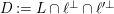 $D:=L\cap \ell ^{\bot }\cap {\ell ^{\prime }}^{\bot }$
. Equipped with the restriction of
$D:=L\cap \ell ^{\bot }\cap {\ell ^{\prime }}^{\bot }$
. Equipped with the restriction of
 $\langle \cdot ,\cdot \rangle$
,
$\langle \cdot ,\cdot \rangle$
,
 $D$
is a definite Hermitian lattice of signature
$D$
is a definite Hermitian lattice of signature
 $(0,n)$
. Denote by
$(0,n)$
. Denote by
 $W=W_{\mathbf{k}}$
the subspace
$W=W_{\mathbf{k}}$
the subspace
 $D\otimes _{{\mathcal{O}}_{\mathbf{k}}}\mathbf{k}$
, and let
$D\otimes _{{\mathcal{O}}_{\mathbf{k}}}\mathbf{k}$
, and let
 $W_{\mathbb{C}}=W\otimes _{\mathbf{k}}\mathbb{C}$
.
$W_{\mathbb{C}}=W\otimes _{\mathbf{k}}\mathbb{C}$
.
Now, an affine model for
 $\mathbb{D}$
, called the Siegel domain model, is given by the following generalized upper-half-plane:
$\mathbb{D}$
, called the Siegel domain model, is given by the following generalized upper-half-plane:
 $$\begin{eqnarray}{\mathcal{H}}_{\ell ,\ell ^{\prime }}=\{(\unicode[STIX]{x1D70F},\unicode[STIX]{x1D70E})\in \mathbb{C}\times W_{\mathbb{C}};2\Im (\unicode[STIX]{x1D70F})|\unicode[STIX]{x1D6FF}_{\mathbf{k}}||\langle \ell ,\ell ^{\prime }\rangle |^{2}>-\langle \unicode[STIX]{x1D70E},\unicode[STIX]{x1D70E}\rangle \}.\end{eqnarray}$$
For
 $(\unicode[STIX]{x1D70F},\unicode[STIX]{x1D70E})\in {\mathcal{H}}_{\ell ,\ell ^{\prime }}$
, we set
$(\unicode[STIX]{x1D70F},\unicode[STIX]{x1D70E})\in {\mathcal{H}}_{\ell ,\ell ^{\prime }}$
, we set
 $$\begin{eqnarray}z=z(\unicode[STIX]{x1D70F},\unicode[STIX]{x1D70E}):=\ell ^{\prime }-\unicode[STIX]{x1D6FF}_{\boldsymbol{ k}}\unicode[STIX]{x1D70F}\langle \ell ^{\prime },\ell \rangle \ell +\unicode[STIX]{x1D70E}.\end{eqnarray}$$
Clearly, under the canonical projection
 $\unicode[STIX]{x1D70B}_{V}:V_{\mathbb{C}}\rightarrow \mathbb{P}V_{\mathbb{C}}$
, we have
$\unicode[STIX]{x1D70B}_{V}:V_{\mathbb{C}}\rightarrow \mathbb{P}V_{\mathbb{C}}$
, we have
 $\unicode[STIX]{x1D70B}_{V}(z)\in {\mathcal{C}}$
for all
$\unicode[STIX]{x1D70B}_{V}(z)\in {\mathcal{C}}$
for all
 $(\unicode[STIX]{x1D70F},\unicode[STIX]{x1D70E})\in {\mathcal{H}}_{\ell ,\ell ^{\prime }}$
. Conversely, every
$(\unicode[STIX]{x1D70F},\unicode[STIX]{x1D70E})\in {\mathcal{H}}_{\ell ,\ell ^{\prime }}$
. Conversely, every
 $[v]\in {\mathcal{C}}$
contains a representative of the form
$[v]\in {\mathcal{C}}$
contains a representative of the form
 $z(\unicode[STIX]{x1D70F},\unicode[STIX]{x1D70E})$
for some pair
$z(\unicode[STIX]{x1D70F},\unicode[STIX]{x1D70E})$
for some pair
 $(\unicode[STIX]{x1D70F},\unicode[STIX]{x1D70E})\in {\mathcal{H}}_{\ell ,\ell ^{\prime }}$
. Usually, in the following, since
$(\unicode[STIX]{x1D70F},\unicode[STIX]{x1D70E})\in {\mathcal{H}}_{\ell ,\ell ^{\prime }}$
. Usually, in the following, since
 $\ell$
and
$\ell$
and
 $\ell ^{\prime }$
are fixed, we shall simply write
$\ell ^{\prime }$
are fixed, we shall simply write
 ${\mathcal{H}}={\mathcal{H}}_{\ell ,\ell ^{\prime }}$
.
${\mathcal{H}}={\mathcal{H}}_{\ell ,\ell ^{\prime }}$
.
The isotropic line
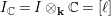 $I_{\mathbb{C}}=I\otimes _{\mathbf{k}}\mathbb{C}=[\ell ]$
corresponds to the cusp at infinity of
$I_{\mathbb{C}}=I\otimes _{\mathbf{k}}\mathbb{C}=[\ell ]$
corresponds to the cusp at infinity of
 ${\mathcal{H}}$
.
${\mathcal{H}}$
.
2.3 Stabilizer of the cusp
Next, we describe the stabilizer in
 $\unicode[STIX]{x1D6E4}$
of the cusp
$\unicode[STIX]{x1D6E4}$
of the cusp
 $[\ell ]$
. Consider the following transformations corresponding to elements of
$[\ell ]$
. Consider the following transformations corresponding to elements of
 $\text{SU}(V)$
:
$\text{SU}(V)$
:
 $$\begin{eqnarray}\displaystyle & \displaystyle [h,0]:v\mapsto v-\langle v,\ell \rangle \unicode[STIX]{x1D6FF}_{\mathbf{k}}h\ell \quad \text{for }h\in \mathbb{Q}, & \displaystyle\end{eqnarray}$$
 $$\begin{eqnarray}\displaystyle & \displaystyle [0,t]:v\mapsto v+\langle v,\ell \rangle t-\langle v,t\rangle \ell -{\textstyle \frac{1}{2}}\langle v,\ell \rangle \langle t,t\rangle \ell \quad \text{for }t\in W. & \displaystyle\end{eqnarray}$$
Clearly, these transformations stabilize the isotropic subspace
 $\mathbf{k}\ell$
. Their action on
$\mathbf{k}\ell$
. Their action on
 ${\mathcal{H}}$
is given as follows:
${\mathcal{H}}$
is given as follows:
 $$\begin{eqnarray}\displaystyle & \displaystyle [h,0]:(\unicode[STIX]{x1D70F},\unicode[STIX]{x1D70E})\mapsto (\unicode[STIX]{x1D70F}+h,\unicode[STIX]{x1D70E}), & \displaystyle \nonumber\\ \displaystyle & \displaystyle \hspace{0.0pt}[0,t]:(\unicode[STIX]{x1D70F},\unicode[STIX]{x1D70E})\mapsto \biggl(\unicode[STIX]{x1D70F}+\frac{\langle \unicode[STIX]{x1D70E},t\rangle }{\unicode[STIX]{x1D6FF}_{\mathbf{k}}\langle \ell ^{\prime },\ell \rangle }+\frac{1}{2}\frac{\langle t,t\rangle }{\unicode[STIX]{x1D6FF}_{\mathbf{k}}},\unicode[STIX]{x1D70E}+\langle \ell ^{\prime },\ell \rangle t\biggr). & \displaystyle \nonumber\end{eqnarray}$$
The Heisenberg group attached to
 $\ell$
, denoted
$\ell$
, denoted
 $\text{Heis}_{\ell }$
, is the set of pairs
$\text{Heis}_{\ell }$
, is the set of pairs
 $[h,t]$
with group law given by
$[h,t]$
with group law given by
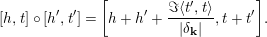 $$\begin{eqnarray}[h,t]\circ [h^{\prime },t^{\prime }]=\biggl[h+h^{\prime }+\frac{\Im \langle t^{\prime },t\rangle }{|\unicode[STIX]{x1D6FF}_{\mathbf{k}}|},t+t^{\prime }\biggr].\end{eqnarray}$$
Here, we follow the convention that
 $([h,t]\circ [h^{\prime },t^{\prime }])v=[h,t]([h^{\prime },t^{\prime }]\,v)$
for
$([h,t]\circ [h^{\prime },t^{\prime }])v=[h,t]([h^{\prime },t^{\prime }]\,v)$
for
 $v\in V_{\mathbf{k}}$
. The center of the Heisenberg group consists of transformations of type (2).
$v\in V_{\mathbf{k}}$
. The center of the Heisenberg group consists of transformations of type (2).
We denote by
 $\unicode[STIX]{x1D6E4}_{\ell }$
the subgroup of
$\unicode[STIX]{x1D6E4}_{\ell }$
the subgroup of
 $\unicode[STIX]{x1D6E4}$
given by the intersection
$\unicode[STIX]{x1D6E4}$
given by the intersection
 $\unicode[STIX]{x1D6E4}\cap \text{Heis}_{\ell }$
, its center we denote by
$\unicode[STIX]{x1D6E4}\cap \text{Heis}_{\ell }$
, its center we denote by
 $\unicode[STIX]{x1D6E4}_{\ell ,T}$
. The full stabilizer of the cusp in
$\unicode[STIX]{x1D6E4}_{\ell ,T}$
. The full stabilizer of the cusp in
 $\unicode[STIX]{x1D6E4}$
is given by the semidirect product
$\unicode[STIX]{x1D6E4}$
is given by the semidirect product
 $$\begin{eqnarray}\unicode[STIX]{x1D6E4}_{\ell }\ltimes (\text{U}(W)\cap \unicode[STIX]{x1D6E4})=\operatorname{Stab}_{\unicode[STIX]{x1D6E4}}(\ell ).\end{eqnarray}$$
Note that
 $\unicode[STIX]{x1D6E4}_{\ell }$
has finite index in the stabilizer. The elements of
$\unicode[STIX]{x1D6E4}_{\ell }$
has finite index in the stabilizer. The elements of
 $\unicode[STIX]{x1D6E4}_{\ell }$
can be described as follows (this is well-known):
$\unicode[STIX]{x1D6E4}_{\ell }$
can be described as follows (this is well-known):
Remark 2.1. Suppose
 $\unicode[STIX]{x1D6E4}$
is a unitary modular group and let
$\unicode[STIX]{x1D6E4}$
is a unitary modular group and let
 $\unicode[STIX]{x1D6E4}_{\ell }=\unicode[STIX]{x1D6E4}\cap \text{Heis}_{\ell }$
. Then there exist a positive rational number
$\unicode[STIX]{x1D6E4}_{\ell }=\unicode[STIX]{x1D6E4}\cap \text{Heis}_{\ell }$
. Then there exist a positive rational number
 $N_{\ell ,\unicode[STIX]{x1D6E4}}$
and a lattice
$N_{\ell ,\unicode[STIX]{x1D6E4}}$
and a lattice
 $D_{\ell ,\unicode[STIX]{x1D6E4}}$
of finite index in
$D_{\ell ,\unicode[STIX]{x1D6E4}}$
of finite index in
 $D$
, such that
$D$
, such that
 $[h,t]\in \unicode[STIX]{x1D6E4}_{\ell }$
for all
$[h,t]\in \unicode[STIX]{x1D6E4}_{\ell }$
for all
 $h\in N_{\ell ,\unicode[STIX]{x1D6E4}}\mathbb{Z}$
,
$h\in N_{\ell ,\unicode[STIX]{x1D6E4}}\mathbb{Z}$
,
 $t\in D_{\ell ,\unicode[STIX]{x1D6E4}}$
, and that
$t\in D_{\ell ,\unicode[STIX]{x1D6E4}}$
, and that
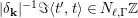 $|\unicode[STIX]{x1D6FF}_{\mathbf{k}}|^{-1}\Im \langle t^{\prime },t\rangle \in N_{\ell ,\unicode[STIX]{x1D6E4}}\mathbb{Z}$
for all
$|\unicode[STIX]{x1D6FF}_{\mathbf{k}}|^{-1}\Im \langle t^{\prime },t\rangle \in N_{\ell ,\unicode[STIX]{x1D6E4}}\mathbb{Z}$
for all
 $t,t^{\prime }\in D_{\ell ,\unicode[STIX]{x1D6E4}}$
.
$t,t^{\prime }\in D_{\ell ,\unicode[STIX]{x1D6E4}}$
.
2.4 Boundary components
The modular variety
 $X_{\unicode[STIX]{x1D6E4}}$
is given by the quotient
$X_{\unicode[STIX]{x1D6E4}}$
is given by the quotient
 $$\begin{eqnarray}\unicode[STIX]{x1D6E4}\backslash \mathbb{D}\simeq \unicode[STIX]{x1D6E4}\backslash \text{U}(V)(\mathbb{R})/{\mathcal{K}}\simeq \unicode[STIX]{x1D6E4}\backslash {\mathcal{H}}.\end{eqnarray}$$
Note that
 $X_{\unicode[STIX]{x1D6E4}}$
is noncompact. The usual Baily–Borel compactification
$X_{\unicode[STIX]{x1D6E4}}$
is noncompact. The usual Baily–Borel compactification
 $X_{\unicode[STIX]{x1D6E4},BB}^{\ast }$
is obtained by introducing a topology and a complex structure on the quotient
$X_{\unicode[STIX]{x1D6E4},BB}^{\ast }$
is obtained by introducing a topology and a complex structure on the quotient
 $$\begin{eqnarray}\unicode[STIX]{x1D6E4}\backslash ({\mathcal{H}}\cup \{I_{\mathbb{R}};I\in \text{Iso}(V)\}).\end{eqnarray}$$
We sketch this for the cusp at infinity, defined by
 $[\ell ]$
. The following sets constitute a system of neighborhoods of the cusp
$[\ell ]$
. The following sets constitute a system of neighborhoods of the cusp
 $$\begin{eqnarray}U_{\unicode[STIX]{x1D716}}(\ell )=\left\{[z]\in {\mathcal{C}};\frac{\langle z,z\rangle }{|\langle z,\ell \rangle |^{2}}|\langle \ell ^{\prime },\ell \rangle |^{2}>\frac{1}{\unicode[STIX]{x1D716}}\right\}\quad (\unicode[STIX]{x1D716}>0).\end{eqnarray}$$
A subset
 $V$
of
$V$
of
 ${\mathcal{C}}\cup \{[\ell ]\}$
is called open if
${\mathcal{C}}\cup \{[\ell ]\}$
is called open if
 $V\cap {\mathcal{C}}$
is open in the usual sense and further if
$V\cap {\mathcal{C}}$
is open in the usual sense and further if
 $[\ell ]\in V$
implies
$[\ell ]\in V$
implies
 $U_{\unicode[STIX]{x1D716}}(\ell )\subset V$
for some
$U_{\unicode[STIX]{x1D716}}(\ell )\subset V$
for some
 $\unicode[STIX]{x1D716}>0$
.
$\unicode[STIX]{x1D716}>0$
.
Through the quotient topology, this construction yields a topology on
 $\unicode[STIX]{x1D6E4}\backslash ({\mathcal{C}}\cup \{[\ell ]\})$
. The complex structure is defined though the pullback under the canonical projection
$\unicode[STIX]{x1D6E4}\backslash ({\mathcal{C}}\cup \{[\ell ]\})$
. The complex structure is defined though the pullback under the canonical projection
 ${\mathcal{C}}\cap \{I_{\mathbb{R}};I\in \text{Iso}(V)\}\rightarrow X_{\unicode[STIX]{x1D6E4},BB}^{\ast }$
, locally for each cusp, see [Reference Hofmann8] for details. This way, one gets the structure of a normal complex space on
${\mathcal{C}}\cap \{I_{\mathbb{R}};I\in \text{Iso}(V)\}\rightarrow X_{\unicode[STIX]{x1D6E4},BB}^{\ast }$
, locally for each cusp, see [Reference Hofmann8] for details. This way, one gets the structure of a normal complex space on
 $X_{\unicode[STIX]{x1D6E4},BB}^{\ast }$
. In general, however, there are still singularities at the boundary points.
$X_{\unicode[STIX]{x1D6E4},BB}^{\ast }$
. In general, however, there are still singularities at the boundary points.
This difficulty can be avoided by using a toroidal compactification, instead. We recall the construction briefly; see [Reference Hofmann8, Chapter 1.1.5] and, in particular [Reference Bruinier, Howard and Yang5, Section 4.3] for more details. In the following, identify the sets
 $U_{\unicode[STIX]{x1D716}}(\ell )\subset {\mathcal{C}}$
with the corresponding sets of representatives in
$U_{\unicode[STIX]{x1D716}}(\ell )\subset {\mathcal{C}}$
with the corresponding sets of representatives in
 ${\mathcal{H}}_{\ell ,\ell ^{\prime }}$
. Clearly, the Heisenberg group
${\mathcal{H}}_{\ell ,\ell ^{\prime }}$
. Clearly, the Heisenberg group
 $\unicode[STIX]{x1D6E4}_{\ell }$
operates on
$\unicode[STIX]{x1D6E4}_{\ell }$
operates on
 $U_{\unicode[STIX]{x1D716}}(\ell )$
. For sufficiently small
$U_{\unicode[STIX]{x1D716}}(\ell )$
. For sufficiently small
 $\unicode[STIX]{x1D716}$
, there is an open immersion
$\unicode[STIX]{x1D716}$
, there is an open immersion
 $$\begin{eqnarray}\unicode[STIX]{x1D6E4}_{\ell }\backslash U_{\unicode[STIX]{x1D716}}(\ell )\rightarrow X_{\unicode[STIX]{x1D6E4}}.\end{eqnarray}$$
Recall that for the center
 $C(\unicode[STIX]{x1D6E4}_{\ell })=\unicode[STIX]{x1D6E4}_{\ell ,T}$
, we have
$C(\unicode[STIX]{x1D6E4}_{\ell })=\unicode[STIX]{x1D6E4}_{\ell ,T}$
, we have
 $\unicode[STIX]{x1D6E4}_{\ell ,T}\simeq \mathbb{Z}N_{\ell ,\unicode[STIX]{x1D6E4}}$
. We set
$\unicode[STIX]{x1D6E4}_{\ell ,T}\simeq \mathbb{Z}N_{\ell ,\unicode[STIX]{x1D6E4}}$
. We set
 $q_{\ell }:=\exp (2\unicode[STIX]{x1D70B}i\unicode[STIX]{x1D70F}/N_{\ell ,\unicode[STIX]{x1D6E4}})$
. The quotient
$q_{\ell }:=\exp (2\unicode[STIX]{x1D70B}i\unicode[STIX]{x1D70F}/N_{\ell ,\unicode[STIX]{x1D6E4}})$
. The quotient
 $\unicode[STIX]{x1D6E4}_{\ell ,T}\backslash U_{\unicode[STIX]{x1D716}}(\ell )$
can now be viewed as bundle of punctured disks over
$\unicode[STIX]{x1D6E4}_{\ell ,T}\backslash U_{\unicode[STIX]{x1D716}}(\ell )$
can now be viewed as bundle of punctured disks over
 $W_{\mathbb{C}}$
:
$W_{\mathbb{C}}$
:
 $$\begin{eqnarray}V_{\unicode[STIX]{x1D716}}(\ell ):=\unicode[STIX]{x1D6E4}_{\ell ,T}\backslash U_{\unicode[STIX]{x1D716}}(\ell )\simeq \left\{(q_{\ell },\unicode[STIX]{x1D70E});0<|q_{\ell }|<\exp \biggl(\frac{\unicode[STIX]{x1D70B}\langle \unicode[STIX]{x1D70E},\unicode[STIX]{x1D70E}\rangle +\unicode[STIX]{x1D716}^{-1}}{|\unicode[STIX]{x1D6FF}_{\mathbf{k}}|^{2}|\langle \ell ^{\prime },\ell \rangle |^{2}}\biggr)\right\}.\end{eqnarray}$$
Adding the center to each disk, we get the disk bundle
 $$\begin{eqnarray}\widetilde{V_{\unicode[STIX]{x1D716}}}(\ell ):=\left\{(q_{\ell },\unicode[STIX]{x1D70E});|q_{\ell }|<\exp \biggl(\frac{\unicode[STIX]{x1D70B}\langle \unicode[STIX]{x1D70E},\unicode[STIX]{x1D70E}\rangle +\unicode[STIX]{x1D716}^{-1}}{|\unicode[STIX]{x1D6FF}_{\mathbf{k}}|^{2}|\langle \ell ^{\prime },\ell \rangle |^{2}}\biggr)\right\}.\end{eqnarray}$$
The action of
 $\unicode[STIX]{x1D6E4}_{\ell }$
is well-defined at each center, leaving the divisor
$\unicode[STIX]{x1D6E4}_{\ell }$
is well-defined at each center, leaving the divisor
 $q=0$
fixed. Also, if
$q=0$
fixed. Also, if
 $\unicode[STIX]{x1D6E4}$
is sufficiently small, the operation is free, hence we get an open immersion
$\unicode[STIX]{x1D6E4}$
is sufficiently small, the operation is free, hence we get an open immersion
 $$\begin{eqnarray}\unicode[STIX]{x1D6E4}_{\ell }\backslash U_{\unicode[STIX]{x1D716}}(\ell )\rightarrow (\unicode[STIX]{x1D6E4}_{\ell }/\unicode[STIX]{x1D6E4}_{\ell ,T})\backslash \widetilde{V_{\unicode[STIX]{x1D716}}}(\ell ),\end{eqnarray}$$
by which the right-hand side can be glued to
 $X_{\unicode[STIX]{x1D6E4}}$
, yielding a partial compactification. For a point
$X_{\unicode[STIX]{x1D6E4}}$
, yielding a partial compactification. For a point
 $(0,\unicode[STIX]{x1D70E}_{0})\in \widetilde{V_{\unicode[STIX]{x1D716}}}(\ell )$
, we define a system of open sets
$(0,\unicode[STIX]{x1D70E}_{0})\in \widetilde{V_{\unicode[STIX]{x1D716}}}(\ell )$
, we define a system of open sets
 $$\begin{eqnarray}B_{\unicode[STIX]{x1D6FF}}(0,\unicode[STIX]{x1D70E}_{0})=\{(q_{\ell },\unicode[STIX]{x1D70E})\in \widetilde{V_{\unicode[STIX]{x1D716}}}(\ell );\langle \unicode[STIX]{x1D70E}-\unicode[STIX]{x1D70E}_{0},\unicode[STIX]{x1D70E}-\unicode[STIX]{x1D70E}_{0}\rangle <\unicode[STIX]{x1D6FF},|q_{\ell }|<\unicode[STIX]{x1D6FF}\}\quad (\unicode[STIX]{x1D6FF}>0).\end{eqnarray}$$
Under the immersion (6) the images of these sets form a system of open neighborhoods for the boundary point at
 $(0,\unicode[STIX]{x1D70E}_{0})$
.
$(0,\unicode[STIX]{x1D70E}_{0})$
.
Repeating this construction and the gluing procedure for every
 $I\in \unicode[STIX]{x1D6E4}\backslash \text{Iso}(V)$
yields a compactification of
$I\in \unicode[STIX]{x1D6E4}\backslash \text{Iso}(V)$
yields a compactification of
 $X_{\unicode[STIX]{x1D6E4}}$
, which we denote
$X_{\unicode[STIX]{x1D6E4}}$
, which we denote
 $X_{\unicode[STIX]{x1D6E4},\text{tor}}^{\ast }$
.
$X_{\unicode[STIX]{x1D6E4},\text{tor}}^{\ast }$
.
3 The local cohomology group
In the following, let
 $\unicode[STIX]{x1D6E4}$
be a unitary modular group and let
$\unicode[STIX]{x1D6E4}$
be a unitary modular group and let
 $\unicode[STIX]{x1D6E4}_{\ell }\subset \unicode[STIX]{x1D6E4}$
be a Heisenberg group of the form
$\unicode[STIX]{x1D6E4}_{\ell }\subset \unicode[STIX]{x1D6E4}$
be a Heisenberg group of the form
 $\unicode[STIX]{x1D6E4}_{\ell }=N_{\ell ,\unicode[STIX]{x1D6E4}}\mathbb{Z}\rtimes D_{\ell ,\unicode[STIX]{x1D6E4}}$
with
$\unicode[STIX]{x1D6E4}_{\ell }=N_{\ell ,\unicode[STIX]{x1D6E4}}\mathbb{Z}\rtimes D_{\ell ,\unicode[STIX]{x1D6E4}}$
with
 $N_{\ell ,\unicode[STIX]{x1D6E4}}\in \mathbb{Q}_{{>}0}$
and
$N_{\ell ,\unicode[STIX]{x1D6E4}}\in \mathbb{Q}_{{>}0}$
and
 $D_{\ell ,\unicode[STIX]{x1D6E4}}\subseteq D$
as introduced in Remark 2.1. We are interested in the cohomology of
$D_{\ell ,\unicode[STIX]{x1D6E4}}\subseteq D$
as introduced in Remark 2.1. We are interested in the cohomology of
 $\unicode[STIX]{x1D6E4}_{\ell }$
, more specifically the second cohomology group
$\unicode[STIX]{x1D6E4}_{\ell }$
, more specifically the second cohomology group
 $\text{H}^{2}(\unicode[STIX]{x1D6E4}_{\ell },\mathbb{Z})$
.
$\text{H}^{2}(\unicode[STIX]{x1D6E4}_{\ell },\mathbb{Z})$
.
As usual, if
 $G$
is a group acting on an abelian group
$G$
is a group acting on an abelian group
 $A$
, the
$A$
, the
 $n$
th cohomology group is defined as the quotient
$n$
th cohomology group is defined as the quotient
 $$\begin{eqnarray}\text{H}^{n}(G,A)=\frac{\operatorname{ker}(\text{C}^{n}(G,A)\xrightarrow[{}]{\unicode[STIX]{x2202}}\text{C}^{n+1}(G,A))}{\operatorname{im}(\text{C}^{n-1}(G,A)\xrightarrow[{}]{\unicode[STIX]{x2202}}\text{C}^{n}(G,A))},\end{eqnarray}$$
wherein
 $\text{C}^{n}$
is the set of
$\text{C}^{n}$
is the set of
 $n$
-cocycles, consisting of all functions
$n$
-cocycles, consisting of all functions
 $f:G^{n}\rightarrow A$
, and
$f:G^{n}\rightarrow A$
, and
 $\unicode[STIX]{x2202}$
is the coboundary operator. In the present setting,
$\unicode[STIX]{x2202}$
is the coboundary operator. In the present setting,
 $G=\unicode[STIX]{x1D6E4}_{\ell }$
,
$G=\unicode[STIX]{x1D6E4}_{\ell }$
,
 $A=\mathbb{Z}$
and the action of
$A=\mathbb{Z}$
and the action of
 $G$
is trivial.
$G$
is trivial.
Let
 $U_{\unicode[STIX]{x1D716}}(\ell )$
be a neighborhood of the cusp of infinity, as defined in (5) above, with
$U_{\unicode[STIX]{x1D716}}(\ell )$
be a neighborhood of the cusp of infinity, as defined in (5) above, with
 $\unicode[STIX]{x1D716}$
sufficiently small, so that the map in (6) is indeed an open immersion. Further, denote by
$\unicode[STIX]{x1D716}$
sufficiently small, so that the map in (6) is indeed an open immersion. Further, denote by
 ${\mathcal{O}}_{\unicode[STIX]{x1D716}}={\mathcal{O}}_{\unicode[STIX]{x1D716}}(U_{\unicode[STIX]{x1D716}}(\ell ))$
the sheaf of holomorphic functions on
${\mathcal{O}}_{\unicode[STIX]{x1D716}}={\mathcal{O}}_{\unicode[STIX]{x1D716}}(U_{\unicode[STIX]{x1D716}}(\ell ))$
the sheaf of holomorphic functions on
 $U_{\unicode[STIX]{x1D716}}(\ell )$
and by
$U_{\unicode[STIX]{x1D716}}(\ell )$
and by
 ${\mathcal{O}}_{\unicode[STIX]{x1D716}}^{\ast }={\mathcal{O}}_{\unicode[STIX]{x1D716}}(U_{\unicode[STIX]{x1D716}}(\ell ))^{\ast }$
the sheaf of invertible holomorphic functions. The action of
${\mathcal{O}}_{\unicode[STIX]{x1D716}}^{\ast }={\mathcal{O}}_{\unicode[STIX]{x1D716}}(U_{\unicode[STIX]{x1D716}}(\ell ))^{\ast }$
the sheaf of invertible holomorphic functions. The action of
 $\unicode[STIX]{x1D6E4}_{\ell }$
on
$\unicode[STIX]{x1D6E4}_{\ell }$
on
 $U_{\unicode[STIX]{x1D716}}(\ell )$
naturally induces an action on
$U_{\unicode[STIX]{x1D716}}(\ell )$
naturally induces an action on
 ${\mathcal{O}}_{\unicode[STIX]{x1D716}}$
and
${\mathcal{O}}_{\unicode[STIX]{x1D716}}$
and
 ${\mathcal{O}}_{\unicode[STIX]{x1D716}}^{\ast }$
. The exact sequence
${\mathcal{O}}_{\unicode[STIX]{x1D716}}^{\ast }$
. The exact sequence

thus induces an exact sequence of cohomology groups:

The Picard group of
 $\unicode[STIX]{x1D6E4}_{\ell }\backslash U_{\unicode[STIX]{x1D716}}(\ell )$
is given by
$\unicode[STIX]{x1D6E4}_{\ell }\backslash U_{\unicode[STIX]{x1D716}}(\ell )$
is given by
 $\text{H}^{1}(\unicode[STIX]{x1D6E4}_{\ell }\backslash U_{\unicode[STIX]{x1D716}}(\ell ),{\mathcal{O}}_{\unicode[STIX]{x1D716}}^{\ast })$
. Since the open neighborhoods
$\text{H}^{1}(\unicode[STIX]{x1D6E4}_{\ell }\backslash U_{\unicode[STIX]{x1D716}}(\ell ),{\mathcal{O}}_{\unicode[STIX]{x1D716}}^{\ast })$
. Since the open neighborhoods
 $U_{\unicode[STIX]{x1D716}}(\ell )$
are contractible, all analytic line bundles on
$U_{\unicode[STIX]{x1D716}}(\ell )$
are contractible, all analytic line bundles on
 $U_{\unicode[STIX]{x1D716}}(\ell )$
are trivial. Therefore,
$U_{\unicode[STIX]{x1D716}}(\ell )$
are trivial. Therefore,
 $$\begin{eqnarray}\text{Pic}(\unicode[STIX]{x1D6E4}_{\ell }\backslash U_{\unicode[STIX]{x1D716}}(\ell ))=\text{H}^{1}(\unicode[STIX]{x1D6E4}_{\ell },{\mathcal{O}}_{\unicode[STIX]{x1D716}}^{\ast }).\end{eqnarray}$$
Further, let
 ${\mathcal{P}}_{\unicode[STIX]{x1D716}}$
denote the functions in
${\mathcal{P}}_{\unicode[STIX]{x1D716}}$
denote the functions in
 ${\mathcal{O}}_{\unicode[STIX]{x1D716}}$
which are periodic for the action of
${\mathcal{O}}_{\unicode[STIX]{x1D716}}$
which are periodic for the action of
 $N_{\ell ,\unicode[STIX]{x1D6E4}}\mathbb{Z}$
. As
$N_{\ell ,\unicode[STIX]{x1D6E4}}\mathbb{Z}$
. As
 $N_{\ell ,\unicode[STIX]{x1D6E4}}\mathbb{Z}=\unicode[STIX]{x1D6E4}_{\ell ,T}$
is a normal subgroup with
$N_{\ell ,\unicode[STIX]{x1D6E4}}\mathbb{Z}=\unicode[STIX]{x1D6E4}_{\ell ,T}$
is a normal subgroup with
 $\unicode[STIX]{x1D6E4}_{\ell }/N_{\ell ,\unicode[STIX]{x1D6E4}}\mathbb{Z}=D_{\ell ,\unicode[STIX]{x1D6E4}}$
, and since
$\unicode[STIX]{x1D6E4}_{\ell }/N_{\ell ,\unicode[STIX]{x1D6E4}}\mathbb{Z}=D_{\ell ,\unicode[STIX]{x1D6E4}}$
, and since
 $N_{\ell ,\unicode[STIX]{x1D6E4}}\mathbb{Z}\backslash U_{\unicode[STIX]{x1D716}}(\ell )$
is contractible, we have
$N_{\ell ,\unicode[STIX]{x1D6E4}}\mathbb{Z}\backslash U_{\unicode[STIX]{x1D716}}(\ell )$
is contractible, we have
 $\text{H}^{p}(\unicode[STIX]{x1D6E4}_{\ell },{\mathcal{O}}_{\unicode[STIX]{x1D716}})=\text{H}^{p}(D_{\ell ,\unicode[STIX]{x1D6E4}},{\mathcal{P}}_{\unicode[STIX]{x1D716}})$
 $(p=1,2,\ldots )$
. Thus, from the exact sequences in (7) and (8), we get the exact sequence
$(p=1,2,\ldots )$
. Thus, from the exact sequences in (7) and (8), we get the exact sequence
Further, since
 $D_{\ell ,\unicode[STIX]{x1D6E4}}$
is a free group, the following sequence is exact:
$D_{\ell ,\unicode[STIX]{x1D6E4}}$
is a free group, the following sequence is exact:
Whence, from (9) we find the exact sequence
Thus, to study
 $\text{Pic}(\unicode[STIX]{x1D6E4}_{\ell }\backslash U_{\unicode[STIX]{x1D716}}(\ell ))$
we want to examine the structure of
$\text{Pic}(\unicode[STIX]{x1D6E4}_{\ell }\backslash U_{\unicode[STIX]{x1D716}}(\ell ))$
we want to examine the structure of
 $\text{H}^{2}(\unicode[STIX]{x1D6E4}_{\ell },\mathbb{Z})$
.
$\text{H}^{2}(\unicode[STIX]{x1D6E4}_{\ell },\mathbb{Z})$
.
3.1 Bilinear forms in the cohomology
In this subsection, we examine the image of certain bilinear forms in the cohomology. All calculations are carried out using the standard inhomogeneous complex of group cohomology (cf. [Reference Shimura10, Chapter 8]).
Definition 3.1. Consider the set of bilinear forms
 $B:W_{\mathbb{C}}\otimes W_{\mathbb{C}}\rightarrow \mathbb{R}$
, for which there is either a Hermitian form
$B:W_{\mathbb{C}}\otimes W_{\mathbb{C}}\rightarrow \mathbb{R}$
, for which there is either a Hermitian form
 $H$
or a symmetric complex bilinear form
$H$
or a symmetric complex bilinear form
 $G$
such that
$G$
such that
 $B=\Im H$
or
$B=\Im H$
or
 $B=\Im G$
, respectively. Such forms generate a vector space of real bilinear forms on
$B=\Im G$
, respectively. Such forms generate a vector space of real bilinear forms on
 $W_{\mathbb{C}}$
, which we denote
$W_{\mathbb{C}}$
, which we denote
 $\mathsf{BIL}$
. Further, let
$\mathsf{BIL}$
. Further, let
 $\mathsf{BIL}_{\mathbb{Z}}$
denote the set of forms in
$\mathsf{BIL}_{\mathbb{Z}}$
denote the set of forms in
 $\mathsf{BIL}$
which are
$\mathsf{BIL}$
which are
 $\mathbb{Z}$
-valued on the lattice
$\mathbb{Z}$
-valued on the lattice
 $D_{\ell ,\unicode[STIX]{x1D6E4}}$
.
$D_{\ell ,\unicode[STIX]{x1D6E4}}$
.
To a bilinear form in
 $\mathsf{BIL}$
we can associate an element of
$\mathsf{BIL}$
we can associate an element of
 $\text{H}^{2}(\unicode[STIX]{x1D6E4}_{\ell },{\mathcal{O}}_{\unicode[STIX]{x1D716}})$
. Define the two-cocycle in
$\text{H}^{2}(\unicode[STIX]{x1D6E4}_{\ell },{\mathcal{O}}_{\unicode[STIX]{x1D716}})$
. Define the two-cocycle in
 $C^{2}(\unicode[STIX]{x1D6E4}_{\ell },{\mathcal{O}}_{\unicode[STIX]{x1D716}})$
by setting
$C^{2}(\unicode[STIX]{x1D6E4}_{\ell },{\mathcal{O}}_{\unicode[STIX]{x1D716}})$
by setting
 $$\begin{eqnarray}B([h,t],[h^{\prime },t^{\prime }]):=B(t,t^{\prime })\quad ([h,t],[h^{\prime },t^{\prime }]\in \unicode[STIX]{x1D6E4}_{\ell }).\end{eqnarray}$$
The class
 $[B]$
of this cocycle is the image of
$[B]$
of this cocycle is the image of
 $B$
in the cohomology. For
$B$
in the cohomology. For
 $B\in \mathsf{BIL}_{\mathbb{Z}}$
we also define a two-cocycle in
$B\in \mathsf{BIL}_{\mathbb{Z}}$
we also define a two-cocycle in
 $\text{C}^{2}(\unicode[STIX]{x1D6E4}_{\ell },\mathbb{Z})$
and the attached element in
$\text{C}^{2}(\unicode[STIX]{x1D6E4}_{\ell },\mathbb{Z})$
and the attached element in
 $\text{H}^{2}(\unicode[STIX]{x1D6E4}_{\ell },\mathbb{Z})$
. Thus, composing with the natural map
$\text{H}^{2}(\unicode[STIX]{x1D6E4}_{\ell },\mathbb{Z})$
. Thus, composing with the natural map
 $\text{H}^{2}(\unicode[STIX]{x1D6E4}_{\ell },\mathbb{Z})\rightarrow \text{H}^{2}(\unicode[STIX]{x1D6E4}_{\ell },{\mathcal{O}}_{\unicode[STIX]{x1D716}})$
from (7) we have a sequence
$\text{H}^{2}(\unicode[STIX]{x1D6E4}_{\ell },\mathbb{Z})\rightarrow \text{H}^{2}(\unicode[STIX]{x1D6E4}_{\ell },{\mathcal{O}}_{\unicode[STIX]{x1D716}})$
from (7) we have a sequence

The composition of the two maps in (12) is just the restriction to
 $\mathsf{BIL}_{\mathbb{Z}}$
of the map
$\mathsf{BIL}_{\mathbb{Z}}$
of the map
 $\mathsf{BIL}\rightarrow \text{H}^{2}(\unicode[STIX]{x1D6E4}_{\ell },{\mathcal{O}}_{\unicode[STIX]{x1D716}})$
defined by (11). It turns out that the sequence is exact:
$\mathsf{BIL}\rightarrow \text{H}^{2}(\unicode[STIX]{x1D6E4}_{\ell },{\mathcal{O}}_{\unicode[STIX]{x1D716}})$
defined by (11). It turns out that the sequence is exact:
Proposition 3.1. The image of
 $\mathsf{BIL}$
in
$\mathsf{BIL}$
in
 $\text{H}^{2}(\unicode[STIX]{x1D6E4}_{\ell },{\mathcal{O}}_{\unicode[STIX]{x1D716}})$
vanishes.
$\text{H}^{2}(\unicode[STIX]{x1D6E4}_{\ell },{\mathcal{O}}_{\unicode[STIX]{x1D716}})$
vanishes.
Proof. In the following, let
 $B$
denote an element of
$B$
denote an element of
 $\mathsf{BIL}$
. Clearly, it suffices to consider the following two cases: either
$\mathsf{BIL}$
. Clearly, it suffices to consider the following two cases: either
 $B$
arises from a Hermitian form or
$B$
arises from a Hermitian form or
 $B$
arises from a bilinear form.
$B$
arises from a bilinear form.
(1) Let
 $H:W_{\mathbb{C}}\times W_{\mathbb{C}}\longrightarrow \mathbb{C}$
be a Hermitian form. Consider the following one-cocycle in
$\text{C}^{1}(\unicode[STIX]{x1D6E4}_{\ell },{\mathcal{O}}_{\unicode[STIX]{x1D716}})$
: Its image under the coboundary map it given by$$\begin{eqnarray}u([h,t],z)=\frac{1}{2i}\biggl[\frac{2}{\langle \ell ^{\prime },\ell \rangle }H(\unicode[STIX]{x1D70E},t)+H(t,t)\biggr].\end{eqnarray}$$
Thus, we see that$$\begin{eqnarray}\displaystyle \unicode[STIX]{x2202}u([h,t],[h^{\prime },t^{\prime }],z) & = & \displaystyle [h,t]u([h^{\prime },t^{\prime }],z)-u([h,t][h^{\prime },t^{\prime }],z)+u([h,t])\nonumber\\ \displaystyle & = & \displaystyle \frac{1}{2i}(2H(t,t^{\prime })-H(t,t^{\prime })-H(t^{\prime },t)).\nonumber\end{eqnarray}$$
$B=\Im H$
is indeed trivialized by a cochain. Hence, its image
$\text{H}^{2}(\unicode[STIX]{x1D6E4}_{\ell },{\mathcal{O}}_{\unicode[STIX]{x1D716}})$
vanishes
$H:W_{\mathbb{C}}\times W_{\mathbb{C}}\longrightarrow \mathbb{C}$
be a Hermitian form. Consider the following one-cocycle in
$\text{C}^{1}(\unicode[STIX]{x1D6E4}_{\ell },{\mathcal{O}}_{\unicode[STIX]{x1D716}})$
: Its image under the coboundary map it given by$$\begin{eqnarray}u([h,t],z)=\frac{1}{2i}\biggl[\frac{2}{\langle \ell ^{\prime },\ell \rangle }H(\unicode[STIX]{x1D70E},t)+H(t,t)\biggr].\end{eqnarray}$$
Thus, we see that$$\begin{eqnarray}\displaystyle \unicode[STIX]{x2202}u([h,t],[h^{\prime },t^{\prime }],z) & = & \displaystyle [h,t]u([h^{\prime },t^{\prime }],z)-u([h,t][h^{\prime },t^{\prime }],z)+u([h,t])\nonumber\\ \displaystyle & = & \displaystyle \frac{1}{2i}(2H(t,t^{\prime })-H(t,t^{\prime })-H(t^{\prime },t)).\nonumber\end{eqnarray}$$
$B=\Im H$
is indeed trivialized by a cochain. Hence, its image
$\text{H}^{2}(\unicode[STIX]{x1D6E4}_{\ell },{\mathcal{O}}_{\unicode[STIX]{x1D716}})$
vanishes(2) Let
$G:W_{\mathbb{C}}\times W_{\mathbb{C}}\longrightarrow \mathbb{C}$
be a symmetric complex bilinear form. We consider the following one-cocycle valued in
${\mathcal{O}}_{\unicode[STIX]{x1D716}}$
: Its image under the coboundary map is given by$$\begin{eqnarray}u([h,t],z)=\frac{i}{2}\biggl(\frac{1}{\langle \ell ^{\prime },\ell \rangle }G(\unicode[STIX]{x1D70E},t)+\frac{1}{2}\overline{G(t,t)}\biggr).\end{eqnarray}$$
Thus$$\begin{eqnarray}\displaystyle \unicode[STIX]{x2202}u([h,t],[h^{\prime },t^{\prime }],z) & = & \displaystyle \frac{1}{2i}\biggl(G(t^{\prime },t)-\frac{1}{2}\overline{G(t,t^{\prime })}-\frac{1}{2}\overline{G(t^{\prime },t)}\biggr)\nonumber\\ \displaystyle & = & \displaystyle \frac{1}{2i}(G(t^{\prime },t)-\overline{G(t^{\prime },t)}).\nonumber\end{eqnarray}$$
$B=\Im G$
is trivialized by a cochain, and
$[B]=0$
in
$\text{H}^{2}(\unicode[STIX]{x1D6E4}_{\ell },{\mathcal{O}}_{\unicode[STIX]{x1D716}})$
. ◻


Remark 3.1. We note that under a map of the type defined in (11), the real parts of sesquilinear forms have vanishing image in
 $\text{H}^{2}(\unicode[STIX]{x1D6E4}_{\ell },{\mathcal{O}}_{\unicode[STIX]{x1D716}})$
, too. The proof is quite similar.
$\text{H}^{2}(\unicode[STIX]{x1D6E4}_{\ell },{\mathcal{O}}_{\unicode[STIX]{x1D716}})$
, too. The proof is quite similar.
Now that we know the sequence (12) to be exact, we study the first map
 $\mathsf{BIL}_{\mathbb{Z}}\rightarrow \text{H}^{2}(\unicode[STIX]{x1D6E4}_{\ell },\mathbb{Z})$
. It is far from being injective. The following lemma and its proof are essentially due to Freitag, a sketch is contained in (E. Freitag, personal communication, 2007).
$\mathsf{BIL}_{\mathbb{Z}}\rightarrow \text{H}^{2}(\unicode[STIX]{x1D6E4}_{\ell },\mathbb{Z})$
. It is far from being injective. The following lemma and its proof are essentially due to Freitag, a sketch is contained in (E. Freitag, personal communication, 2007).
Lemma 3.1. The kernel of the map
 $\mathsf{BIL}_{\mathbb{Z}}\rightarrow \text{H}^{2}(\unicode[STIX]{x1D6E4}_{\ell },\mathbb{Z})$
is the cyclic group generated by the antisymmetric bilinear form
$\mathsf{BIL}_{\mathbb{Z}}\rightarrow \text{H}^{2}(\unicode[STIX]{x1D6E4}_{\ell },\mathbb{Z})$
is the cyclic group generated by the antisymmetric bilinear form
 $$\begin{eqnarray}\frac{1}{N_{\ell ,\unicode[STIX]{x1D6E4}}}\frac{\Im \langle \cdot ,\cdot \rangle }{|\unicode[STIX]{x1D6FF}_{\mathbf{k}}|}.\end{eqnarray}$$
In particular, the image of an element
 $B\in \mathsf{BIL}_{\mathbb{Z}}$
is a torsion element in
$B\in \mathsf{BIL}_{\mathbb{Z}}$
is a torsion element in
 $\text{H}^{2}(\unicode[STIX]{x1D6E4}_{\ell },\mathbb{Z})$
if and if
$\text{H}^{2}(\unicode[STIX]{x1D6E4}_{\ell },\mathbb{Z})$
if and if
 $B$
and
$B$
and
 $|\unicode[STIX]{x1D6FF}_{\mathbf{k}}|^{-1}\Im \langle \cdot ,\cdot \rangle$
are linear dependent over
$|\unicode[STIX]{x1D6FF}_{\mathbf{k}}|^{-1}\Im \langle \cdot ,\cdot \rangle$
are linear dependent over
 $\mathbb{Z}$
.
$\mathbb{Z}$
.
Proof. The proof uses a transgression map, which we introduce next. First note that, since the action of
 $\mathbb{Z}$
is trivial, the map
$\mathbb{Z}$
is trivial, the map
 $\mathsf{BIL}_{\mathbb{Z}}\rightarrow \text{H}^{2}(\unicode[STIX]{x1D6E4}_{\ell },\mathbb{Z})$
factors over
$\mathsf{BIL}_{\mathbb{Z}}\rightarrow \text{H}^{2}(\unicode[STIX]{x1D6E4}_{\ell },\mathbb{Z})$
factors over
 $\text{H}^{2}(D_{\ell ,\unicode[STIX]{x1D6E4}},\mathbb{Z})=\text{H}^{2}((\unicode[STIX]{x1D6E4}_{\ell }/N_{\ell ,\unicode[STIX]{x1D6E4}}\mathbb{Z}),\mathbb{Z})$
. With Proposition 3.1 we have:
$\text{H}^{2}(D_{\ell ,\unicode[STIX]{x1D6E4}},\mathbb{Z})=\text{H}^{2}((\unicode[STIX]{x1D6E4}_{\ell }/N_{\ell ,\unicode[STIX]{x1D6E4}}\mathbb{Z}),\mathbb{Z})$
. With Proposition 3.1 we have:

Now, the transgression
 $\operatorname{tg}$
is defined as the map for which the sequence
$\operatorname{tg}$
is defined as the map for which the sequence

becomes exact. Thus, the kernel of the map into
 $\text{H}^{2}(\unicode[STIX]{x1D6E4}_{\ell },\mathbb{Z})$
is generated by the image of the identity map
$\text{H}^{2}(\unicode[STIX]{x1D6E4}_{\ell },\mathbb{Z})$
is generated by the image of the identity map
 $\mathbf{1}:\mathbb{Z}\rightarrow \mathbb{Z}$
under
$\mathbf{1}:\mathbb{Z}\rightarrow \mathbb{Z}$
under
 $\operatorname{tg}$
. The image
$\operatorname{tg}$
. The image
 $\operatorname{tg}(\mathbf{1})$
is represented by a coboundary
$\operatorname{tg}(\mathbf{1})$
is represented by a coboundary
 $(t,t^{\prime })\mapsto (\unicode[STIX]{x2202}u)([\cdot ,t],[\cdot ,t^{\prime }])$
, with a one-cochain
$(t,t^{\prime })\mapsto (\unicode[STIX]{x2202}u)([\cdot ,t],[\cdot ,t^{\prime }])$
, with a one-cochain
 $u:\unicode[STIX]{x1D6E4}_{\ell }\rightarrow \mathbb{Z}$
, which has to satisfy two conditions:
$u:\unicode[STIX]{x1D6E4}_{\ell }\rightarrow \mathbb{Z}$
, which has to satisfy two conditions:
(1)
$u([N_{\ell ,\unicode[STIX]{x1D6E4}}\,h,0])=h$
for all
$h\in \mathbb{Z}$
and(2)
$(\unicode[STIX]{x2202}u)([h,t],[h^{\prime },t^{\prime }])$
does not depend on
$h$
or
$h^{\prime }$
.


A suitable
 $u$
is obtained by setting
$u$
is obtained by setting
 $u([N_{\ell ,\unicode[STIX]{x1D6E4}}h,t]):=h$
. We get
$u([N_{\ell ,\unicode[STIX]{x1D6E4}}h,t]):=h$
. We get
 $$\begin{eqnarray}\displaystyle (\unicode[STIX]{x2202}u)([h,t],[h^{\prime },t^{\prime }]) & = & \displaystyle [h,t]u([h^{\prime },t^{\prime }])-u([h,t][h^{\prime },t^{\prime }])+u([h,t])\nonumber\\ \displaystyle & = & \displaystyle -\frac{1}{N_{\ell ,\unicode[STIX]{x1D6E4}}}\frac{\Im \langle t^{\prime },t\rangle }{|\unicode[STIX]{x1D6FF}_{\mathbf{k}}|}.\nonumber\end{eqnarray}$$
Hence,
 $\operatorname{tg}(\mathbf{1})$
is represented by the cocycle
$\operatorname{tg}(\mathbf{1})$
is represented by the cocycle
 $$\begin{eqnarray}(t,t^{\prime })\longmapsto \frac{1}{N_{\ell ,\unicode[STIX]{x1D6E4}}}\frac{\Im \langle t,t^{\prime }\rangle }{|\unicode[STIX]{x1D6FF}_{\mathbf{k}}|},\end{eqnarray}$$
any integer multiple of which is then contained in the kernel. Thus, for any
 $B\in \mathsf{BIL}_{\mathbb{Z}}$
the image
$B\in \mathsf{BIL}_{\mathbb{Z}}$
the image
 $[B]$
is a torsion element precisely if it is linear dependent to
$[B]$
is a torsion element precisely if it is linear dependent to
 $\operatorname{tg}(\mathbf{1})$
over
$\operatorname{tg}(\mathbf{1})$
over
 $\mathbb{Z}$
.◻
$\mathbb{Z}$
.◻
The linear dependence condition in the lemma can more conveniently be formulated thus: if
 $B\in \mathsf{BIL}_{\mathbb{Z}}$
, the image is a torsion element if and only if there is a rational number
$B\in \mathsf{BIL}_{\mathbb{Z}}$
, the image is a torsion element if and only if there is a rational number
 $Q$
, such that for all
$Q$
, such that for all
 $t,t^{\prime }\in D_{\ell ,\unicode[STIX]{x1D6E4}}$
, the following equation holds:
$t,t^{\prime }\in D_{\ell ,\unicode[STIX]{x1D6E4}}$
, the following equation holds:
 $$\begin{eqnarray}B(t,t^{\prime })-Q\frac{\Im \langle t,t^{\prime }\rangle }{|\unicode[STIX]{x1D6FF}_{\mathbf{k}}|}=0.\end{eqnarray}$$
Since
 $D_{\ell ,\unicode[STIX]{x1D6E4}}$
has full rank in
$D_{\ell ,\unicode[STIX]{x1D6E4}}$
has full rank in
 $W_{\mathbf{k}}$
, by linear extension, equivalently, the equation holds for all
$W_{\mathbf{k}}$
, by linear extension, equivalently, the equation holds for all
 $t,t^{\prime }\in W$
; similarly for all
$t,t^{\prime }\in W$
; similarly for all
 $t,t^{\prime }\in W_{\mathbb{C}}$
. As an example for this, we give an application to Hermitian forms.
$t,t^{\prime }\in W_{\mathbb{C}}$
. As an example for this, we give an application to Hermitian forms.
Remark 3.2. Let
 $H$
be a
$H$
be a
 $\mathbf{k}$
-valued Hermitian form on
$\mathbf{k}$
-valued Hermitian form on
 $W_{\mathbf{k}}$
, and assume that
$W_{\mathbf{k}}$
, and assume that
 ${|\unicode[STIX]{x1D6FF}_{\mathbf{k}}|}^{-1}\Im H\in \mathsf{BIL}_{\mathbb{Z}}$
. Further assume that
${|\unicode[STIX]{x1D6FF}_{\mathbf{k}}|}^{-1}\Im H\in \mathsf{BIL}_{\mathbb{Z}}$
. Further assume that
 $H$
is linear in its left argument (otherwise, invert the sign in the equation below).
$H$
is linear in its left argument (otherwise, invert the sign in the equation below).
Then, the map
 $H\mapsto {|\unicode[STIX]{x1D6FF}_{\mathbf{k}}|}^{-1}\Im H$
defines a torsion element in
$H\mapsto {|\unicode[STIX]{x1D6FF}_{\mathbf{k}}|}^{-1}\Im H$
defines a torsion element in
 $\text{H}^{2}(\unicode[STIX]{x1D6E4}_{\ell },\mathbb{Z})$
if and only if the following equation holds for all
$\text{H}^{2}(\unicode[STIX]{x1D6E4}_{\ell },\mathbb{Z})$
if and only if the following equation holds for all
 $t,t^{\prime }\in D_{\ell ,\unicode[STIX]{x1D6E4}}$
:
$t,t^{\prime }\in D_{\ell ,\unicode[STIX]{x1D6E4}}$
:
 $$\begin{eqnarray}H(t,t^{\prime })+\frac{\operatorname{Tr}H}{n}\Im \langle t,t^{\prime }\rangle =0,\end{eqnarray}$$
where the trace
 $\operatorname{Tr}$
is taken over a normalized orthogonal basis for
$\operatorname{Tr}$
is taken over a normalized orthogonal basis for
 $\langle \cdot ,\cdot \rangle$
.
$\langle \cdot ,\cdot \rangle$
.
Proof. Taking the imaginary part of (15), we see that indeed, if the equation holds,
 $\Im H$
is a rational multiple of
$\Im H$
is a rational multiple of
 $\Im \langle \cdot ,\cdot \rangle$
and thus
$\Im \langle \cdot ,\cdot \rangle$
and thus
 ${|\unicode[STIX]{x1D6FF}_{\mathbf{k}}|}^{-1}\Im H$
defines a torsion element by the lemma.
${|\unicode[STIX]{x1D6FF}_{\mathbf{k}}|}^{-1}\Im H$
defines a torsion element by the lemma.
Conversely, assume that the image is a torsion element in
 $\text{H}^{2}(\unicode[STIX]{x1D6E4}_{\ell },\mathbb{Z})$
. Then, by the lemma, the form has to be linear dependent to
$\text{H}^{2}(\unicode[STIX]{x1D6E4}_{\ell },\mathbb{Z})$
. Then, by the lemma, the form has to be linear dependent to
 ${|\unicode[STIX]{x1D6FF}_{\mathbf{k}}|}^{-1}\Im \langle \cdot ,\cdot \rangle$
and satisfies an equation of the form (14). Since by linear extension, the equation holds for all
${|\unicode[STIX]{x1D6FF}_{\mathbf{k}}|}^{-1}\Im \langle \cdot ,\cdot \rangle$
and satisfies an equation of the form (14). Since by linear extension, the equation holds for all
 $t,t^{\prime }\in W_{\mathbb{C}}$
, we may replace
$t,t^{\prime }\in W_{\mathbb{C}}$
, we may replace
 $t$
by a purely imaginary multiple. The resulting equation, equivalent to the first, is the following:
$t$
by a purely imaginary multiple. The resulting equation, equivalent to the first, is the following:
 $$\begin{eqnarray}\Re H(t,t^{\prime })-Q\cdot \Re \langle t,t^{\prime }\rangle =0,\end{eqnarray}$$
valid for all
 $t,t^{\prime }\in W_{\mathbb{C}}$
. Whence by linear combination of the two equations, we find
$t,t^{\prime }\in W_{\mathbb{C}}$
. Whence by linear combination of the two equations, we find
 $H(t,t^{\prime })=Q\langle t,t^{\prime }\rangle$
for all
$H(t,t^{\prime })=Q\langle t,t^{\prime }\rangle$
for all
 $t,t^{\prime }\in W_{\mathbb{C}}$
. To determine the factor of proportionality
$t,t^{\prime }\in W_{\mathbb{C}}$
. To determine the factor of proportionality
 $Q$
, we take the trace. We have
$Q$
, we take the trace. We have
 $\operatorname{Tr}\langle \cdot ,\cdot \rangle \mid _{W_{\mathbb{C}}}=-n$
, and get
$\operatorname{Tr}\langle \cdot ,\cdot \rangle \mid _{W_{\mathbb{C}}}=-n$
, and get
 $Q=-(1/n)\operatorname{Tr}H$
.◻
$Q=-(1/n)\operatorname{Tr}H$
.◻
4 Local Heegner divisors and Borcherds products
Our main interest here is to study the contribution of Heegner divisors to the local Picard group. For this purpose, we introduce local Borcherds products and, with their help, calculate the Chern classes of local Heegner divisors in
 $\text{H}^{2}(\unicode[STIX]{x1D6E4}_{\ell },\mathbb{Z})$
. Then, we apply the cohomological results from Section 3.
$\text{H}^{2}(\unicode[STIX]{x1D6E4}_{\ell },\mathbb{Z})$
. Then, we apply the cohomological results from Section 3.
The local Picard group
 $\text{Pic}(X_{\unicode[STIX]{x1D6E4}},\ell )$
is defined as the direct limit of the Picard groups on the regular loci (in the Baily–Borel compactification
$\text{Pic}(X_{\unicode[STIX]{x1D6E4}},\ell )$
is defined as the direct limit of the Picard groups on the regular loci (in the Baily–Borel compactification
 $X_{\unicode[STIX]{x1D6E4},BB}^{\ast }$
) of the open neighborhoods
$X_{\unicode[STIX]{x1D6E4},BB}^{\ast }$
) of the open neighborhoods
 $U_{\unicode[STIX]{x1D716}}(\ell )$
of the cusp attached to
$U_{\unicode[STIX]{x1D716}}(\ell )$
of the cusp attached to
 $\ell$
:
$\ell$
:
 $$\begin{eqnarray}\text{Pic}(X_{\unicode[STIX]{x1D6E4}},\ell )=\varinjlim \text{Pic}(U_{\unicode[STIX]{x1D716}}^{\text{reg}}).\end{eqnarray}$$
Up to torsion, we can describe this local Picard group through the direct system
 $\text{Pic}(\unicode[STIX]{x1D6E4}_{\ell }\backslash U_{\unicode[STIX]{x1D716}}(\ell ))$
, as
$\text{Pic}(\unicode[STIX]{x1D6E4}_{\ell }\backslash U_{\unicode[STIX]{x1D716}}(\ell ))$
, as
 $\unicode[STIX]{x1D6E4}_{\ell }$
has finite index in the stabilizer of the cusp,
$\unicode[STIX]{x1D6E4}_{\ell }$
has finite index in the stabilizer of the cusp,
 $\operatorname{Stab}_{\unicode[STIX]{x1D6E4}}(\ell )$
. As the quotient
$\operatorname{Stab}_{\unicode[STIX]{x1D6E4}}(\ell )$
. As the quotient
 $\operatorname{Stab}_{\unicode[STIX]{x1D6E4}}(\ell )/\unicode[STIX]{x1D6E4}_{\ell }$
operates on the direct limit
$\operatorname{Stab}_{\unicode[STIX]{x1D6E4}}(\ell )/\unicode[STIX]{x1D6E4}_{\ell }$
operates on the direct limit
 $\varinjlim \text{Pic}(\unicode[STIX]{x1D6E4}_{\ell }\backslash U_{\unicode[STIX]{x1D716}}(\ell ))$
, for the invariant part, one has
$\varinjlim \text{Pic}(\unicode[STIX]{x1D6E4}_{\ell }\backslash U_{\unicode[STIX]{x1D716}}(\ell ))$
, for the invariant part, one has
 $$\begin{eqnarray}\text{Pic}(X_{\unicode[STIX]{x1D6E4}},\ell )\otimes \mathbb{Q}=(\varinjlim \text{Pic}(\unicode[STIX]{x1D6E4}_{\ell }\backslash U_{\unicode[STIX]{x1D716}}(\ell ))\otimes \mathbb{Q})^{\operatorname{Stab}_{\unicode[STIX]{x1D6E4}}(\ell )/\unicode[STIX]{x1D6E4}_{\ell }}.\end{eqnarray}$$
Thus, to describe the position of a local divisor up to torsion, it suffices to work with the Picard group
 $\text{Pic}(\unicode[STIX]{x1D6E4}_{\ell }\backslash U_{\unicode[STIX]{x1D716}}(\ell ))$
for a fixed (sufficiently small)
$\text{Pic}(\unicode[STIX]{x1D6E4}_{\ell }\backslash U_{\unicode[STIX]{x1D716}}(\ell ))$
for a fixed (sufficiently small)
 $\unicode[STIX]{x1D716}>0$
.
$\unicode[STIX]{x1D716}>0$
.
Remark 4.1. Replacing the Baily–Borel compactification
 $X_{\unicode[STIX]{x1D6E4},BB}^{\ast }$
with the toroidal compactification
$X_{\unicode[STIX]{x1D6E4},BB}^{\ast }$
with the toroidal compactification
 $X_{\unicode[STIX]{x1D6E4},\text{tor}}^{\ast }$
, the system of open neighborhoods
$X_{\unicode[STIX]{x1D6E4},\text{tor}}^{\ast }$
, the system of open neighborhoods
 $U_{\unicode[STIX]{x1D716}}$
is replaced by the system of open neighborhoods
$U_{\unicode[STIX]{x1D716}}$
is replaced by the system of open neighborhoods
 $\widetilde{V_{\unicode[STIX]{x1D716}}}(\ell )$
with the operation of
$\widetilde{V_{\unicode[STIX]{x1D716}}}(\ell )$
with the operation of
 $\unicode[STIX]{x1D6E4}_{\ell }/\unicode[STIX]{x1D6E4}_{\ell ,T}$
, and one can look at the Picard groups
$\unicode[STIX]{x1D6E4}_{\ell }/\unicode[STIX]{x1D6E4}_{\ell ,T}$
, and one can look at the Picard groups
 $\text{Pic}(\unicode[STIX]{x1D6E4}_{\ell }/\unicode[STIX]{x1D6E4}_{\ell ,T}\backslash \widetilde{V_{\unicode[STIX]{x1D716}}}(\ell ))$
. The main difference here is, that now, the divisor of
$\text{Pic}(\unicode[STIX]{x1D6E4}_{\ell }/\unicode[STIX]{x1D6E4}_{\ell ,T}\backslash \widetilde{V_{\unicode[STIX]{x1D716}}}(\ell ))$
. The main difference here is, that now, the divisor of
 $\{q_{\ell }=0\}$
is a nontrivial element of the Picard group. A function with this divisor is
$\{q_{\ell }=0\}$
is a nontrivial element of the Picard group. A function with this divisor is
 $q_{\ell }=e(N_{\ell ,\unicode[STIX]{x1D6E4}}^{-1}\unicode[STIX]{x1D70F})$
. Note that the Chern class of
$q_{\ell }=e(N_{\ell ,\unicode[STIX]{x1D6E4}}^{-1}\unicode[STIX]{x1D70F})$
. Note that the Chern class of
 $\{q_{\ell }=0\}$
is precisely
$\{q_{\ell }=0\}$
is precisely
 $(N_{\ell ,\unicode[STIX]{x1D6E4}}|\unicode[STIX]{x1D6FF}_{\mathbf{k}}|)^{-1}\Im \langle t,t^{\prime }\rangle$
.
$(N_{\ell ,\unicode[STIX]{x1D6E4}}|\unicode[STIX]{x1D6FF}_{\mathbf{k}}|)^{-1}\Im \langle t,t^{\prime }\rangle$
.
4.1 Local Heegner divisors
First, we recall the usual definition of Heegner divisors on
 ${\mathcal{H}}$
(cf. [Reference Hofmann9, Section 6]), and introduce local Heegner divisors in the neighborhoods
${\mathcal{H}}$
(cf. [Reference Hofmann9, Section 6]), and introduce local Heegner divisors in the neighborhoods
 $U_{\unicode[STIX]{x1D716}}(\ell )$
of the cusp
$U_{\unicode[STIX]{x1D716}}(\ell )$
of the cusp
 $[\ell ]$
.
$[\ell ]$
.
Let
 $\unicode[STIX]{x1D706}\in L^{\prime }$
be a lattice vector of negative norm, that is
$\unicode[STIX]{x1D706}\in L^{\prime }$
be a lattice vector of negative norm, that is
 $\langle \unicode[STIX]{x1D706},\unicode[STIX]{x1D706}\rangle <0$
. The (primitive) Heegner divisor
$\langle \unicode[STIX]{x1D706},\unicode[STIX]{x1D706}\rangle <0$
. The (primitive) Heegner divisor
 $\mathbf{H}(\unicode[STIX]{x1D706})$
attached to
$\mathbf{H}(\unicode[STIX]{x1D706})$
attached to
 $\unicode[STIX]{x1D706}$
is a divisor on
$\unicode[STIX]{x1D706}$
is a divisor on
 ${\mathcal{H}}$
given by
${\mathcal{H}}$
given by
 $$\begin{eqnarray}\mathbf{H}(\unicode[STIX]{x1D706}):=\{(\unicode[STIX]{x1D70F},\unicode[STIX]{x1D70E})\in {\mathcal{H}};\langle \unicode[STIX]{x1D706},z(\unicode[STIX]{x1D70F},\unicode[STIX]{x1D70E})\rangle =0\},\end{eqnarray}$$
with
 $z(\unicode[STIX]{x1D70F},\unicode[STIX]{x1D70E})=\ell ^{\prime }-\unicode[STIX]{x1D70F}\unicode[STIX]{x1D6FF}_{\mathbf{k}}\langle \ell ,\ell ^{\prime }\rangle \ell +\unicode[STIX]{x1D70E}$
(see Section 2.2). Clearly, the divisor
$z(\unicode[STIX]{x1D70F},\unicode[STIX]{x1D70E})=\ell ^{\prime }-\unicode[STIX]{x1D70F}\unicode[STIX]{x1D6FF}_{\mathbf{k}}\langle \ell ,\ell ^{\prime }\rangle \ell +\unicode[STIX]{x1D70E}$
(see Section 2.2). Clearly, the divisor
 $\mathbf{H}(\unicode[STIX]{x1D706})$
intersects
$\mathbf{H}(\unicode[STIX]{x1D706})$
intersects
 $U_{\unicode[STIX]{x1D716}}(\ell )$
for every
$U_{\unicode[STIX]{x1D716}}(\ell )$
for every
 $\unicode[STIX]{x1D716}>0$
, if and only if
$\unicode[STIX]{x1D716}>0$
, if and only if
 $\langle \unicode[STIX]{x1D706},\ell \rangle =0$
. In the following, we denote by
$\langle \unicode[STIX]{x1D706},\ell \rangle =0$
. In the following, we denote by
 $\ell ^{\bot }$
the (orthogonal) complement of
$\ell ^{\bot }$
the (orthogonal) complement of
 $\ell$
with respect to
$\ell$
with respect to
 $\langle \cdot ,\cdot \rangle$
.
$\langle \cdot ,\cdot \rangle$
.
Thus, let
 $\unicode[STIX]{x1D706}\in L^{\prime }\cap \ell ^{\bot }$
. Then,
$\unicode[STIX]{x1D706}\in L^{\prime }\cap \ell ^{\bot }$
. Then,
 $\unicode[STIX]{x1D706}=\unicode[STIX]{x1D706}_{\ell }\ell +\unicode[STIX]{x1D706}_{D}$
with
$\unicode[STIX]{x1D706}=\unicode[STIX]{x1D706}_{\ell }\ell +\unicode[STIX]{x1D706}_{D}$
with
 $\unicode[STIX]{x1D706}_{D}\in W_{\mathbf{k}}$
and
$\unicode[STIX]{x1D706}_{D}\in W_{\mathbf{k}}$
and
 $\mathbf{H}(\unicode[STIX]{x1D706})$
is given by an equation of the form
$\mathbf{H}(\unicode[STIX]{x1D706})$
is given by an equation of the form
 $$\begin{eqnarray}\unicode[STIX]{x1D706}_{\ell }\langle \ell ,\ell ^{\prime }\rangle +\langle \unicode[STIX]{x1D706}_{D},\unicode[STIX]{x1D70E}\rangle =0.\end{eqnarray}$$
Consider the orbit of
 $\unicode[STIX]{x1D706}$
under
$\unicode[STIX]{x1D706}$
under
 $\unicode[STIX]{x1D6E4}_{\ell }$
. Since
$\unicode[STIX]{x1D6E4}_{\ell }$
. Since
 $\unicode[STIX]{x1D6E4}$
is a modular group, the Heisenberg group
$\unicode[STIX]{x1D6E4}$
is a modular group, the Heisenberg group
 $\unicode[STIX]{x1D6E4}_{\ell }$
operates trivially on the discriminant group
$\unicode[STIX]{x1D6E4}_{\ell }$
operates trivially on the discriminant group
 $L^{\prime }/L$
and thus
$L^{\prime }/L$
and thus
 $[h,t]\unicode[STIX]{x1D706}\equiv \unicode[STIX]{x1D706}\hspace{0.6em}({\rm mod}\hspace{0.2em}L)$
for all
$[h,t]\unicode[STIX]{x1D706}\equiv \unicode[STIX]{x1D706}\hspace{0.6em}({\rm mod}\hspace{0.2em}L)$
for all
 $[h,t]\in \unicode[STIX]{x1D6E4}_{\ell }$
. Also, since
$[h,t]\in \unicode[STIX]{x1D6E4}_{\ell }$
. Also, since
 $\unicode[STIX]{x1D706}\in \ell ^{\bot }$
, it remains fixed under
$\unicode[STIX]{x1D706}\in \ell ^{\bot }$
, it remains fixed under
 $[h,0]$
for all
$[h,0]$
for all
 $h\in N_{\ell ,\unicode[STIX]{x1D6E4}}\mathbb{Z}$
, and
$h\in N_{\ell ,\unicode[STIX]{x1D6E4}}\mathbb{Z}$
, and
 $\unicode[STIX]{x1D6E4}_{\ell ,T}$
acts trivially.
$\unicode[STIX]{x1D6E4}_{\ell ,T}$
acts trivially.
For an Eichler element
 $[0,t]$
with
$[0,t]$
with
 $t\in D_{\ell ,\unicode[STIX]{x1D6E4}}$
, we have
$t\in D_{\ell ,\unicode[STIX]{x1D6E4}}$
, we have
 $$\begin{eqnarray}[0,t]\unicode[STIX]{x1D706}=\unicode[STIX]{x1D706}-\langle \unicode[STIX]{x1D706}_{D},t\rangle \ell =(\unicode[STIX]{x1D706}_{\ell }-\langle \unicode[STIX]{x1D706}_{D},t\rangle )\ell +\unicode[STIX]{x1D706}_{D}.\end{eqnarray}$$
Thus, the orbit of
 $\unicode[STIX]{x1D706}$
under
$\unicode[STIX]{x1D706}$
under
 $\unicode[STIX]{x1D6E4}_{\ell }/\unicode[STIX]{x1D6E4}_{\ell ,T}\simeq D_{\ell ,\unicode[STIX]{x1D6E4}}$
is given by
$\unicode[STIX]{x1D6E4}_{\ell }/\unicode[STIX]{x1D6E4}_{\ell ,T}\simeq D_{\ell ,\unicode[STIX]{x1D6E4}}$
is given by
 $\unicode[STIX]{x1D706}-\mathfrak{T}\ell$
, where
$\unicode[STIX]{x1D706}-\mathfrak{T}\ell$
, where
 $\mathfrak{T}$
denotes the set
$\mathfrak{T}$
denotes the set
 $$\begin{eqnarray}\mathfrak{T}=\mathfrak{T}(\unicode[STIX]{x1D706}):=\{\langle \unicode[STIX]{x1D706},t\rangle ;t\in D_{\ell ,\unicode[STIX]{x1D6E4}}\}.\end{eqnarray}$$
Note that
 $\mathfrak{T}\subseteq \mathfrak{d}_{\mathbf{k}}^{-1}$
(as a fractional ideal), since
$\mathfrak{T}\subseteq \mathfrak{d}_{\mathbf{k}}^{-1}$
(as a fractional ideal), since
 $D_{\ell ,\unicode[STIX]{x1D6E4}}\subseteq D$
.
$D_{\ell ,\unicode[STIX]{x1D6E4}}\subseteq D$
.
Hence, the group
 $\unicode[STIX]{x1D6E4}_{\ell }$
operates on the set
$\unicode[STIX]{x1D6E4}_{\ell }$
operates on the set
 $\unicode[STIX]{x1D706}+\mathfrak{d}_{\mathbf{k}}^{-1}\ell$
with only finitely many orbits and thus, the divisor
$\unicode[STIX]{x1D706}+\mathfrak{d}_{\mathbf{k}}^{-1}\ell$
with only finitely many orbits and thus, the divisor
 $$\begin{eqnarray}\mathbf{H}_{\infty }(\unicode[STIX]{x1D706}):=\mathop{\sum }_{\unicode[STIX]{x1D6FC}\in \mathfrak{d}_{\mathbf{k}}^{-1}}\mathbf{H}(\unicode[STIX]{x1D706}+\unicode[STIX]{x1D6FC}\ell )\end{eqnarray}$$
is invariant under
 $\unicode[STIX]{x1D6E4}_{\ell }$
and defines an element of
$\unicode[STIX]{x1D6E4}_{\ell }$
and defines an element of
 $\operatorname{Div}(\unicode[STIX]{x1D6E4}_{\ell }\backslash U_{\unicode[STIX]{x1D716}}(\ell ))$
.
$\operatorname{Div}(\unicode[STIX]{x1D6E4}_{\ell }\backslash U_{\unicode[STIX]{x1D716}}(\ell ))$
.
Heegner divisors with index
Now, let
 $\unicode[STIX]{x1D6FD}\in L^{\prime }/L$
be an element of the discriminant group and
$\unicode[STIX]{x1D6FD}\in L^{\prime }/L$
be an element of the discriminant group and
 $m$
a negative integer. Then, the Heegner divisor of index
$m$
a negative integer. Then, the Heegner divisor of index
 $(\unicode[STIX]{x1D6FD},m)$
, defined as the (locally finite) sum
$(\unicode[STIX]{x1D6FD},m)$
, defined as the (locally finite) sum
 $$\begin{eqnarray}\mathbf{H}(\unicode[STIX]{x1D6FD},m)=\mathop{\sum }_{\substack{ \unicode[STIX]{x1D706}\in L^{\prime } \\ q(\unicode[STIX]{x1D706})=m \\ \unicode[STIX]{x1D706}+L=\unicode[STIX]{x1D6FD}}}\mathbf{H}(\unicode[STIX]{x1D706}),\end{eqnarray}$$
is a
 $\unicode[STIX]{x1D6E4}$
-invariant divisor on
$\unicode[STIX]{x1D6E4}$
-invariant divisor on
 ${\mathcal{H}}$
. Under the canonical projection
${\mathcal{H}}$
. Under the canonical projection
 $\mathbf{H}(\unicode[STIX]{x1D6FD},m)$
is the inverse image of a divisor on
$\mathbf{H}(\unicode[STIX]{x1D6FD},m)$
is the inverse image of a divisor on
 $X_{\unicode[STIX]{x1D6E4}}$
. Also note that
$X_{\unicode[STIX]{x1D6E4}}$
. Also note that
 $\mathbf{H}(\unicode[STIX]{x1D6FD},m)=\mathbf{H}(-\unicode[STIX]{x1D6FD},m)$
.
$\mathbf{H}(\unicode[STIX]{x1D6FD},m)=\mathbf{H}(-\unicode[STIX]{x1D6FD},m)$
.
Through the open immersion
 $\unicode[STIX]{x1D6E4}_{\ell }\backslash U_{\unicode[STIX]{x1D716}}(\ell ){\hookrightarrow}\unicode[STIX]{x1D6E4}\backslash {\mathcal{H}}=X_{\unicode[STIX]{x1D6E4}}$
from Section 2.4, the inclusion
$\unicode[STIX]{x1D6E4}_{\ell }\backslash U_{\unicode[STIX]{x1D716}}(\ell ){\hookrightarrow}\unicode[STIX]{x1D6E4}\backslash {\mathcal{H}}=X_{\unicode[STIX]{x1D6E4}}$
from Section 2.4, the inclusion
 $U_{\unicode[STIX]{x1D716}}(\ell )\subset {\mathcal{H}}$
and the projection maps, we get a commutative diagram
$U_{\unicode[STIX]{x1D716}}(\ell )\subset {\mathcal{H}}$
and the projection maps, we get a commutative diagram

We denote by
 $\mathbf{H}_{\ell }(\unicode[STIX]{x1D6FD},m)$
the image in
$\mathbf{H}_{\ell }(\unicode[STIX]{x1D6FD},m)$
the image in
 $\operatorname{Div}(\unicode[STIX]{x1D6E4}_{\ell }\backslash U_{\unicode[STIX]{x1D716}}(\ell ))$
of the divisor
$\operatorname{Div}(\unicode[STIX]{x1D6E4}_{\ell }\backslash U_{\unicode[STIX]{x1D716}}(\ell ))$
of the divisor
 $\mathbf{H}(\unicode[STIX]{x1D6FD},m)\in \operatorname{Div}(X_{\unicode[STIX]{x1D6E4}})$
. The corresponding
$\mathbf{H}(\unicode[STIX]{x1D6FD},m)\in \operatorname{Div}(X_{\unicode[STIX]{x1D6E4}})$
. The corresponding
 $\unicode[STIX]{x1D6E4}_{\ell }$
-invariant divisor in
$\unicode[STIX]{x1D6E4}_{\ell }$
-invariant divisor in
 $\operatorname{Div}(U_{\unicode[STIX]{x1D716}}(\ell ))$
is also denoted by
$\operatorname{Div}(U_{\unicode[STIX]{x1D716}}(\ell ))$
is also denoted by
 $\mathbf{H}_{\ell }(\unicode[STIX]{x1D6FD},m)$
.
$\mathbf{H}_{\ell }(\unicode[STIX]{x1D6FD},m)$
.
For sufficiently small
 $\unicode[STIX]{x1D716}$
, the divisor
$\unicode[STIX]{x1D716}$
, the divisor
 $\mathbf{H}_{\ell }(\unicode[STIX]{x1D6FD},m)$
is given by the restriction to
$\mathbf{H}_{\ell }(\unicode[STIX]{x1D6FD},m)$
is given by the restriction to
 $U_{\unicode[STIX]{x1D716}}(\ell )$
of the sum on the right-hand side of (19). Then, only
$U_{\unicode[STIX]{x1D716}}(\ell )$
of the sum on the right-hand side of (19). Then, only
 $\unicode[STIX]{x1D706}$
’s perpendicular to
$\unicode[STIX]{x1D706}$
’s perpendicular to
 $\ell$
contribute. In particular, if
$\ell$
contribute. In particular, if
 $\mathbf{H}_{\ell }(\unicode[STIX]{x1D6FD},m)$
is nonzero, then
$\mathbf{H}_{\ell }(\unicode[STIX]{x1D6FD},m)$
is nonzero, then
 $\unicode[STIX]{x1D6FD}$
is contained in the subgroup
$\unicode[STIX]{x1D6FD}$
is contained in the subgroup
 $$\begin{eqnarray}\displaystyle {\mathcal{L}} & := & \displaystyle \{\!\unicode[STIX]{x1D6FE}\in L^{\prime }/L;2\Re \langle \unicode[STIX]{x1D6FE},\ell \rangle \equiv 0\hspace{0.2em}{\rm mod}\hspace{0.2em}M_{1}\nonumber\\ \displaystyle & & \displaystyle \quad \text{and }|\unicode[STIX]{x1D6FF}_{\mathbf{k}}|\Im \langle \unicode[STIX]{x1D6FE},\ell \rangle \equiv 0\hspace{0.2em}{\rm mod}\hspace{0.2em}M_{2}\!\}\subseteq L^{\prime }/L,\nonumber\end{eqnarray}$$
where
 $M_{1}$
,
$M_{1}$
,
 $M_{2}$
are the unique integers given by
$M_{2}$
are the unique integers given by
 $2\Re \langle L,\ell \rangle =M_{1}\mathbb{Z}$
and by
$2\Re \langle L,\ell \rangle =M_{1}\mathbb{Z}$
and by
 $|\unicode[STIX]{x1D6FF}_{\mathbf{k}}|\Im \langle L,\ell \rangle =M_{2}\mathbb{Z}$
.
$|\unicode[STIX]{x1D6FF}_{\mathbf{k}}|\Im \langle L,\ell \rangle =M_{2}\mathbb{Z}$
.
With
 $\unicode[STIX]{x1D6FD}\in {\mathcal{L}}$
the local divisor
$\unicode[STIX]{x1D6FD}\in {\mathcal{L}}$
the local divisor
 $\mathbf{H}_{\ell }(\unicode[STIX]{x1D6FD},m)$
can be written in the form
$\mathbf{H}_{\ell }(\unicode[STIX]{x1D6FD},m)$
can be written in the form
 $$\begin{eqnarray}\mathbf{H}_{\ell }(\unicode[STIX]{x1D6FD},m)=\mathop{\sum }_{\substack{ \unicode[STIX]{x1D705}\in D \\ q(\unicode[STIX]{x1D705}+\dot{\unicode[STIX]{x1D6FD}})=m}}\mathbf{H}_{\infty }(\unicode[STIX]{x1D705}+\dot{\unicode[STIX]{x1D6FD}}).\end{eqnarray}$$
Here, we adopt the notation of [Reference Bruinier and Freitag4, Section 4], by which
 $\dot{\unicode[STIX]{x1D6FD}}$
denotes a representative of
$\dot{\unicode[STIX]{x1D6FD}}$
denotes a representative of
 $\unicode[STIX]{x1D6FD}$
with
$\unicode[STIX]{x1D6FD}$
with
 $\dot{\unicode[STIX]{x1D6FD}}\in L^{\prime }\cap \ell ^{\bot }$
, fixed once and for all for every
$\dot{\unicode[STIX]{x1D6FD}}\in L^{\prime }\cap \ell ^{\bot }$
, fixed once and for all for every
 $\unicode[STIX]{x1D6FD}\in {\mathcal{L}}$
. Note that a surjective homomorphism is given by
$\unicode[STIX]{x1D6FD}\in {\mathcal{L}}$
. Note that a surjective homomorphism is given by
 $$\begin{eqnarray}\unicode[STIX]{x1D70B}:{\mathcal{L}}\longrightarrow D^{\prime }/D,\qquad \unicode[STIX]{x1D6FD}\longmapsto \dot{\unicode[STIX]{x1D6FD}}_{D},\end{eqnarray}$$
where
 $\dot{\unicode[STIX]{x1D6FD}}_{D}$
denotes the definite part of
$\dot{\unicode[STIX]{x1D6FD}}_{D}$
denotes the definite part of
 $\dot{\unicode[STIX]{x1D6FD}}$
.
$\dot{\unicode[STIX]{x1D6FD}}$
.
4.2 Local Borcherds products
In this section, our aim is to use local Borcherds products to describe the position of Heegner divisors in the cohomology. Given a lattice vector
 $\unicode[STIX]{x1D706}$
of negative norm with
$\unicode[STIX]{x1D706}$
of negative norm with
 $\unicode[STIX]{x1D706}\in L^{\prime }\cap \ell ^{\bot }$
we can realize the local Heegner divisor attached to
$\unicode[STIX]{x1D706}\in L^{\prime }\cap \ell ^{\bot }$
we can realize the local Heegner divisor attached to
 $\unicode[STIX]{x1D706}$
through an infinite product with factors of the form
$\unicode[STIX]{x1D706}$
through an infinite product with factors of the form
 $(1-e(\langle z,[0,t]\unicode[STIX]{x1D706}\rangle ))$
with
$(1-e(\langle z,[0,t]\unicode[STIX]{x1D706}\rangle ))$
with
 $[0,t]\in \unicode[STIX]{x1D6E4}_{\ell ,T}$
.
$[0,t]\in \unicode[STIX]{x1D6E4}_{\ell ,T}$
.
If for the Heegner divisor
 $\mathbf{H}_{\infty }(\unicode[STIX]{x1D706})$
as in (18), we set
$\mathbf{H}_{\infty }(\unicode[STIX]{x1D706})$
as in (18), we set
 $$\begin{eqnarray}\mathop{\prod }_{\unicode[STIX]{x1D6FD}\in \mathfrak{d}_{\mathbf{k}}^{-1}}[1-e(\unicode[STIX]{x1D70E}(\unicode[STIX]{x1D6FD})\langle z,\unicode[STIX]{x1D706}-\unicode[STIX]{x1D6FD}\ell \rangle )],\quad \text{with }\unicode[STIX]{x1D70E}(\unicode[STIX]{x1D6FD})\in \{\pm 1\},\end{eqnarray}$$
we get an infinite product with (zero-)divisor
 $\mathbf{H}(\infty )$
. For
$\mathbf{H}(\infty )$
. For
 $\unicode[STIX]{x1D70E}(\unicode[STIX]{x1D6FD})\equiv 1$
the product would be
$\unicode[STIX]{x1D70E}(\unicode[STIX]{x1D6FD})\equiv 1$
the product would be
 $\unicode[STIX]{x1D6E4}_{\ell }$
-invariant. However, to assure absolute convergence, we must define the sign
$\unicode[STIX]{x1D6E4}_{\ell }$
-invariant. However, to assure absolute convergence, we must define the sign
 $\unicode[STIX]{x1D70E}(\unicode[STIX]{x1D6FD})$
depending on
$\unicode[STIX]{x1D70E}(\unicode[STIX]{x1D6FD})$
depending on
 $\Im \unicode[STIX]{x1D6FD}$
. Then, the product is no longer fully invariant. Instead, the operation of Eichler transformations gives rise to a nontrivial automorphy factor, which we use to determine the position of
$\Im \unicode[STIX]{x1D6FD}$
. Then, the product is no longer fully invariant. Instead, the operation of Eichler transformations gives rise to a nontrivial automorphy factor, which we use to determine the position of
 $\mathbf{H}_{\infty }(\unicode[STIX]{x1D706})$
in the local Picard group.
$\mathbf{H}_{\infty }(\unicode[STIX]{x1D706})$
in the local Picard group.
Assumption.
From here on, we shall require that
 $\langle \ell ,\ell ^{\prime }\rangle =\unicode[STIX]{x1D6FF}_{\mathbf{k}}^{-1}$
.
$\langle \ell ,\ell ^{\prime }\rangle =\unicode[STIX]{x1D6FF}_{\mathbf{k}}^{-1}$
.
We remark that this is not a particularly serious restriction, as under the assumptions concerning
 $\ell$
and
$\ell$
and
 $\ell ^{\prime }$
from Section 2.1, it is always possible to choose
$\ell ^{\prime }$
from Section 2.1, it is always possible to choose
 $\ell ^{\prime }$
suitably.
$\ell ^{\prime }$
suitably.
Now, keeping in mind that
 $\mathfrak{d}_{\mathbf{k}}=\unicode[STIX]{x1D6FF}_{\mathbf{k}}^{-1}{\mathcal{O}}_{\mathbf{k}}$
and
$\mathfrak{d}_{\mathbf{k}}=\unicode[STIX]{x1D6FF}_{\mathbf{k}}^{-1}{\mathcal{O}}_{\mathbf{k}}$
and
 $\overline{{\mathcal{O}}}_{\mathbf{k}}={\mathcal{O}}_{\mathbf{k}}=-{\mathcal{O}}_{\mathbf{k}}$
, we define the local Borcherds products as follows:
$\overline{{\mathcal{O}}}_{\mathbf{k}}={\mathcal{O}}_{\mathbf{k}}=-{\mathcal{O}}_{\mathbf{k}}$
, we define the local Borcherds products as follows:
Definition 4.1. Let
 $\unicode[STIX]{x1D706}\in L^{\prime }$
be a negative-norm lattice vector in the orthogonal complement of
$\unicode[STIX]{x1D706}\in L^{\prime }$
be a negative-norm lattice vector in the orthogonal complement of
 $\ell$
. The local Borcherds product
$\ell$
. The local Borcherds product
 $\unicode[STIX]{x1D6F9}_{\unicode[STIX]{x1D706}}(z)$
attached to
$\unicode[STIX]{x1D6F9}_{\unicode[STIX]{x1D706}}(z)$
attached to
 $\mathbf{H}_{\infty }(\unicode[STIX]{x1D706})$
is defined as
$\mathbf{H}_{\infty }(\unicode[STIX]{x1D706})$
is defined as
 $$\begin{eqnarray}\unicode[STIX]{x1D6F9}_{\unicode[STIX]{x1D706}}(z):=\mathop{\prod }_{\unicode[STIX]{x1D6FC}\in {\mathcal{O}}_{\mathbf{k}}}\biggl[1-e\biggl(\unicode[STIX]{x1D70E}(\Im \unicode[STIX]{x1D6FC})\biggl(\langle z,\unicode[STIX]{x1D706}\rangle +\frac{\unicode[STIX]{x1D6FC}}{|D_{\mathbf{k}}|}\biggr)\biggr)\biggr],\end{eqnarray}$$
with a sign
 $\unicode[STIX]{x1D70E}(\Im \unicode[STIX]{x1D6FC})$
defined as follows:
$\unicode[STIX]{x1D70E}(\Im \unicode[STIX]{x1D6FC})$
defined as follows:
 $$\begin{eqnarray}\unicode[STIX]{x1D70E}(\Im \unicode[STIX]{x1D6FC})=\left\{\begin{array}{@{}ll@{}}1\quad & \text{if }\Im \unicode[STIX]{x1D6FC}\geqslant 0,\\ -1\quad & \text{otherwise.}\end{array}\right.\end{eqnarray}$$
Clearly,
 $\unicode[STIX]{x1D6F9}_{\unicode[STIX]{x1D706}}(z)$
is an absolutely convergent infinite product with divisor
$\unicode[STIX]{x1D6F9}_{\unicode[STIX]{x1D706}}(z)$
is an absolutely convergent infinite product with divisor
 $\mathbf{H}_{\infty }(\unicode[STIX]{x1D706})$
. With
$\mathbf{H}_{\infty }(\unicode[STIX]{x1D706})$
. With
 $\mathfrak{d}_{\mathbf{k}}^{-1}=\unicode[STIX]{x1D6FF}_{\mathbf{k}}^{-1}(\mathbb{Z}+\unicode[STIX]{x1D701}\mathbb{Z})$
, where
$\mathfrak{d}_{\mathbf{k}}^{-1}=\unicode[STIX]{x1D6FF}_{\mathbf{k}}^{-1}(\mathbb{Z}+\unicode[STIX]{x1D701}\mathbb{Z})$
, where
 $\Im \unicode[STIX]{x1D701}=\frac{1}{2}\unicode[STIX]{x1D6FF}_{\mathbf{k}}$
and
$\Im \unicode[STIX]{x1D701}=\frac{1}{2}\unicode[STIX]{x1D6FF}_{\mathbf{k}}$
and
 $2\Re \unicode[STIX]{x1D701}\equiv D_{\mathbf{k}}\hspace{0.6em}({\rm mod}\hspace{0.2em}4)$
, we can write
$2\Re \unicode[STIX]{x1D701}\equiv D_{\mathbf{k}}\hspace{0.6em}({\rm mod}\hspace{0.2em}4)$
, we can write
 $\unicode[STIX]{x1D6F9}_{\unicode[STIX]{x1D706}}(z)$
in the following form
$\unicode[STIX]{x1D6F9}_{\unicode[STIX]{x1D706}}(z)$
in the following form
 $$\begin{eqnarray}\unicode[STIX]{x1D6F9}_{\unicode[STIX]{x1D706}}(z)=\mathop{\prod }_{\substack{ p\hspace{0.2em}{\rm mod}\hspace{0.2em}|D_{\boldsymbol{ k}}| \\ q\in \mathbb{Z}}}\biggl[1-e\biggl(\unicode[STIX]{x1D70E}(q)\biggl(\langle z,\unicode[STIX]{x1D706}\rangle +\frac{1}{|D_{\mathbf{k}}|}(p+\unicode[STIX]{x1D701}q)\biggr)\biggr)\biggr],\end{eqnarray}$$
with
 $\unicode[STIX]{x1D70E}(q)=\operatorname{sign}(q)$
if
$\unicode[STIX]{x1D70E}(q)=\operatorname{sign}(q)$
if
 $q\neq 0$
and
$q\neq 0$
and
 $\unicode[STIX]{x1D70E}(0)=+1$
.
$\unicode[STIX]{x1D70E}(0)=+1$
.
Note that
 $\unicode[STIX]{x1D6F9}_{\unicode[STIX]{x1D706}}$
is invariant under translations in
$\unicode[STIX]{x1D6F9}_{\unicode[STIX]{x1D706}}$
is invariant under translations in
 $\unicode[STIX]{x1D6E4}_{\ell ,T}$
, while the operation of Eichler transformations,
$\unicode[STIX]{x1D6E4}_{\ell ,T}$
, while the operation of Eichler transformations,
 $[0,t]$
with
$[0,t]$
with
 $t\in D_{\ell ,\unicode[STIX]{x1D6E4}}$
, gives rise to the (nontrivial) automorphy factor
$t\in D_{\ell ,\unicode[STIX]{x1D6E4}}$
, gives rise to the (nontrivial) automorphy factor
 $$\begin{eqnarray}J_{\unicode[STIX]{x1D706}}([h,t],z)=\frac{\unicode[STIX]{x1D6F9}_{\unicode[STIX]{x1D706}}([0,t]z)}{\unicode[STIX]{x1D6F9}_{\unicode[STIX]{x1D706}}(z)}\quad ([h,t]\in \unicode[STIX]{x1D6E4}_{\ell }).\end{eqnarray}$$
Proposition 4.1. The automorphy factor
 $J_{\unicode[STIX]{x1D706}}$
attached to
$J_{\unicode[STIX]{x1D706}}$
attached to
 $\mathbf{H}_{\infty }(\unicode[STIX]{x1D706})$
takes the form
$\mathbf{H}_{\infty }(\unicode[STIX]{x1D706})$
takes the form
 $$\begin{eqnarray}J_{\unicode[STIX]{x1D706}}([h,t],z)=e(-2|D_{\mathbf{k}}|\langle z,\unicode[STIX]{x1D706}\rangle \Re \langle t,\unicode[STIX]{x1D706}\rangle -2(\Re \langle t,\unicode[STIX]{x1D706}\rangle )^{2}\unicode[STIX]{x1D701}+\Re \langle t,\unicode[STIX]{x1D706}\rangle (\unicode[STIX]{x1D701}+1)),\end{eqnarray}$$
with
 $\unicode[STIX]{x1D701}$
such that
$\unicode[STIX]{x1D701}$
such that
 ${\mathcal{O}}_{\mathbf{k}}=Z+\unicode[STIX]{x1D701}\mathbb{Z}$
. Note that
${\mathcal{O}}_{\mathbf{k}}=Z+\unicode[STIX]{x1D701}\mathbb{Z}$
. Note that
 $J_{\unicode[STIX]{x1D706}}$
is independent of the choice of
$J_{\unicode[STIX]{x1D706}}$
is independent of the choice of
 $\unicode[STIX]{x1D701}$
.
$\unicode[STIX]{x1D701}$
.
Proof. Since
 $\langle \ell ^{\prime },\ell \rangle =-{\unicode[STIX]{x1D6FF}_{\mathbf{k}}}^{-1}$
, by (3) we have
$\langle \ell ^{\prime },\ell \rangle =-{\unicode[STIX]{x1D6FF}_{\mathbf{k}}}^{-1}$
, by (3) we have
 $\langle [0,t]z,\unicode[STIX]{x1D706}\rangle =\langle z,\unicode[STIX]{x1D706}\rangle -{\unicode[STIX]{x1D6FF}_{\mathbf{k}}}^{-1}\langle t,\unicode[STIX]{x1D706}\rangle$
. Since
$\langle [0,t]z,\unicode[STIX]{x1D706}\rangle =\langle z,\unicode[STIX]{x1D706}\rangle -{\unicode[STIX]{x1D6FF}_{\mathbf{k}}}^{-1}\langle t,\unicode[STIX]{x1D706}\rangle$
. Since
 $\langle t,\unicode[STIX]{x1D706}\rangle =\langle t,\unicode[STIX]{x1D706}_{D}\rangle \in \mathfrak{d}_{\mathbf{k}}^{-1}$
we can write
$\langle t,\unicode[STIX]{x1D706}\rangle =\langle t,\unicode[STIX]{x1D706}_{D}\rangle \in \mathfrak{d}_{\mathbf{k}}^{-1}$
we can write
 $$\begin{eqnarray}\langle [0,t]z,\unicode[STIX]{x1D706}\rangle =\langle z,\unicode[STIX]{x1D706}\rangle +\frac{1}{|D_{\mathbf{k}}|}(r+\unicode[STIX]{x1D701}s),\quad \text{with }r,s\in \mathbb{Z}.\end{eqnarray}$$
We note that
 $s=2\Re \langle t,\unicode[STIX]{x1D706}\rangle$
. Now, after permuting representatives modulo
$s=2\Re \langle t,\unicode[STIX]{x1D706}\rangle$
. Now, after permuting representatives modulo
 $|D_{\mathbf{k}}|$
and a shift in the index
$|D_{\mathbf{k}}|$
and a shift in the index
 $q$
, the automorphy factor from (21) takes the form
$q$
, the automorphy factor from (21) takes the form
 $$\begin{eqnarray}J_{\unicode[STIX]{x1D706}}([h,t],z)=\mathop{\prod }_{p\hspace{0.2em}{\rm mod}\hspace{0.2em}|D_{\mathbf{k}}|}\mathop{\prod }_{q\in \mathbb{Z}}\frac{1-e(\unicode[STIX]{x1D70E}(q-s)(\langle z,\unicode[STIX]{x1D706}\rangle +|D_{\mathbf{k}}|^{-1}(p+q\unicode[STIX]{x1D701})))}{1-e(\unicode[STIX]{x1D70E}(q)(\langle z,\unicode[STIX]{x1D706}\rangle +|D_{\mathbf{k}}|^{-1}(p+q\unicode[STIX]{x1D701})))}.\end{eqnarray}$$
Only factors with
 $\unicode[STIX]{x1D70E}(q-s)\neq \unicode[STIX]{x1D70E}(q)$
contribute to the product. There are two cases: either we have
$\unicode[STIX]{x1D70E}(q-s)\neq \unicode[STIX]{x1D70E}(q)$
contribute to the product. There are two cases: either we have
 $s>q\geqslant 0$
, or
$s>q\geqslant 0$
, or
 $s\leqslant q<0$
. We examine the first case. By applying the elementary identity
$s\leqslant q<0$
. We examine the first case. By applying the elementary identity
 $$\begin{eqnarray}\frac{1-e(-z)}{1-e(z)}=-e(-z).\end{eqnarray}$$
we get
 $$\begin{eqnarray}\displaystyle J_{\unicode[STIX]{x1D706}}([h,t],z) & = & \displaystyle \mathop{\prod }_{p\hspace{0.2em}{\rm mod}\hspace{0.2em}|D_{\mathbf{k}}|}\mathop{\prod }_{0\leqslant q<s}-e\biggl(-\langle z,\unicode[STIX]{x1D706}\rangle -\frac{1}{|D_{\mathbf{k}}|}(p+q\unicode[STIX]{x1D701})\biggr)\nonumber\\ \displaystyle & = & \displaystyle \mathop{\prod }_{p\hspace{0.2em}{\rm mod}\hspace{0.2em}|D_{\mathbf{k}}|}(-1)^{s}e\biggl(-s\langle z,\unicode[STIX]{x1D706}\rangle -\frac{s}{|D_{\mathbf{k}}|}\biggl(p+\frac{s-1}{2}\unicode[STIX]{x1D701}\biggr)\biggr)\nonumber\\ \displaystyle & = & \displaystyle e\biggl(-s|D_{\mathbf{k}}|\langle z,\unicode[STIX]{x1D706}\rangle -\frac{s(s-1)}{2}\unicode[STIX]{x1D701}-\frac{s(|D_{\mathbf{k}}|-1)}{2}+\frac{s|D_{\mathbf{k}}|}{2}\biggr)\nonumber\\ \displaystyle & = & \displaystyle e\biggl(-s|D_{\mathbf{k}}|\langle z,\unicode[STIX]{x1D706}\rangle -\frac{s^{2}}{2}\unicode[STIX]{x1D701}+\frac{s}{2}\unicode[STIX]{x1D701}+\frac{s}{2}\biggr)\nonumber\end{eqnarray}$$
Hence, recalling that
 $s=2\Re \langle t,\unicode[STIX]{x1D706}\rangle$
, we have
$s=2\Re \langle t,\unicode[STIX]{x1D706}\rangle$
, we have
 $$\begin{eqnarray}\displaystyle J_{\unicode[STIX]{x1D706}}([h,t],z) & = & \displaystyle e(\!-2|D_{\mathbf{k}}|\langle z,\unicode[STIX]{x1D706}\rangle \Re \langle t,\unicode[STIX]{x1D706}\rangle \nonumber\\ \displaystyle & & \displaystyle -\,2(\Re \langle t,\unicode[STIX]{x1D706}\rangle )^{2}\unicode[STIX]{x1D701}+\Re \langle t,\unicode[STIX]{x1D706}\rangle \unicode[STIX]{x1D701}+\Re \langle t,\unicode[STIX]{x1D706}\rangle ).\end{eqnarray}$$
We remark that the last term is determined only up to sign, since
 $2\Re \langle t,\unicode[STIX]{x1D706}\rangle \in \mathbb{Z}$
. Finally, we note that as the second term in (23) is a quarter-integer while
$2\Re \langle t,\unicode[STIX]{x1D706}\rangle \in \mathbb{Z}$
. Finally, we note that as the second term in (23) is a quarter-integer while
 $2\Re \unicode[STIX]{x1D701}$
is only determined modulo
$2\Re \unicode[STIX]{x1D701}$
is only determined modulo
 $4$
, the automorphy factor is independent of the choice for
$4$
, the automorphy factor is independent of the choice for
 $\Re \unicode[STIX]{x1D701}$
.
$\Re \unicode[STIX]{x1D701}$
.
The second case (
 $s\leqslant q<0$
) can be treated similarly, yielding the same result for the automorphy factor
$s\leqslant q<0$
) can be treated similarly, yielding the same result for the automorphy factor
 $J_{\unicode[STIX]{x1D706}}([h,t],z)$
.◻
$J_{\unicode[STIX]{x1D706}}([h,t],z)$
.◻
4.3 The Chern class of a Heegner divisor
$\mathbf{H}_{\infty }(\unicode[STIX]{x1D706})$

From the automorphy factor
 $J_{\unicode[STIX]{x1D706}}$
we now determine a two-cocycle representing the Chern class of the Heegner divisor
$J_{\unicode[STIX]{x1D706}}$
we now determine a two-cocycle representing the Chern class of the Heegner divisor
 $\mathbf{H}_{\infty }(\unicode[STIX]{x1D706})$
.
$\mathbf{H}_{\infty }(\unicode[STIX]{x1D706})$
.
Proposition 4.2. The Chern class
 $\unicode[STIX]{x1D6FF}(\mathbf{H}_{\infty }(\unicode[STIX]{x1D706}))$
of the local Heegner divisor
$\unicode[STIX]{x1D6FF}(\mathbf{H}_{\infty }(\unicode[STIX]{x1D706}))$
of the local Heegner divisor
 $\mathbf{H}_{\infty }(\unicode[STIX]{x1D706})$
in
$\mathbf{H}_{\infty }(\unicode[STIX]{x1D706})$
in
 $\text{H}^{2}(\unicode[STIX]{x1D6E4}_{\ell },\mathbb{Z})$
is determined by the cocycle
$\text{H}^{2}(\unicode[STIX]{x1D6E4}_{\ell },\mathbb{Z})$
is determined by the cocycle
 $$\begin{eqnarray}[c_{\unicode[STIX]{x1D706}}]:([h,t][h^{\prime },t^{\prime }])\longmapsto -2|\unicode[STIX]{x1D6FF}_{\boldsymbol{ k}}|\Re \langle t,\unicode[STIX]{x1D706}\rangle \Im \langle t^{\prime },\unicode[STIX]{x1D706}\rangle =\Im (-|\unicode[STIX]{x1D6FF}_{\boldsymbol{ k}}|F_{\unicode[STIX]{x1D706}}(t,t^{\prime })),\end{eqnarray}$$
where
 $F_{\unicode[STIX]{x1D706}}(t,t^{\prime }):=2\Re \langle t,\unicode[STIX]{x1D706}\rangle \langle t^{\prime },\unicode[STIX]{x1D706}\rangle$
.
$F_{\unicode[STIX]{x1D706}}(t,t^{\prime }):=2\Re \langle t,\unicode[STIX]{x1D706}\rangle \langle t^{\prime },\unicode[STIX]{x1D706}\rangle$
.
Proof. To calculate the Chern class, we must realize the connecting homomorphism
 $\unicode[STIX]{x1D6FF}:\text{H}^{1}(\unicode[STIX]{x1D6E4}_{\ell },{\mathcal{O}}_{\unicode[STIX]{x1D716}}^{\ast })\rightarrow \text{H}^{2}(\unicode[STIX]{x1D6E4}_{\ell },\mathbb{Z})$
. Thus, let
$\unicode[STIX]{x1D6FF}:\text{H}^{1}(\unicode[STIX]{x1D6E4}_{\ell },{\mathcal{O}}_{\unicode[STIX]{x1D716}}^{\ast })\rightarrow \text{H}^{2}(\unicode[STIX]{x1D6E4}_{\ell },\mathbb{Z})$
. Thus, let
 $A(g,z)$
be a holomorphic function satisfying
$A(g,z)$
be a holomorphic function satisfying
 $J_{\unicode[STIX]{x1D706}}(g,z)=e(A(g,z))$
and set
$J_{\unicode[STIX]{x1D706}}(g,z)=e(A(g,z))$
and set
 $$\begin{eqnarray}c(g,g^{\prime })=A(gg^{\prime },z)-A(g,g^{\prime }z)-A(g^{\prime },z)\quad \text{for all }g,g^{\prime }\in \unicode[STIX]{x1D6E4}_{\ell }.\end{eqnarray}$$
Then, the two-cocycle defined by the map
 $(g,g)\mapsto c(g,g^{\prime })$
is a representative for the Chern class in
$(g,g)\mapsto c(g,g^{\prime })$
is a representative for the Chern class in
 $\text{H}^{2}(\unicode[STIX]{x1D6E4}_{\ell },\mathbb{Z})$
. Note that while
$\text{H}^{2}(\unicode[STIX]{x1D6E4}_{\ell },\mathbb{Z})$
. Note that while
 $A(g,g^{\prime })$
is not uniquely determined,
$A(g,g^{\prime })$
is not uniquely determined,
 $c(g,g^{\prime })$
is independent of this choice; also, multiplying
$c(g,g^{\prime })$
is independent of this choice; also, multiplying
 $J_{\unicode[STIX]{x1D706}}$
with a trivial automorphy factor changes
$J_{\unicode[STIX]{x1D706}}$
with a trivial automorphy factor changes
 $c(g,g^{\prime })$
only by a coboundary.
$c(g,g^{\prime })$
only by a coboundary.
Clearly, it suffices to calculate
 $c(g,g^{\prime })$
for Eichler transformations
$c(g,g^{\prime })$
for Eichler transformations
 $g=[0,t]$
and
$g=[0,t]$
and
 $g^{\prime }=[0,t^{\prime }]$
. From (24) we see that the last two terms in (23), being linear in
$g^{\prime }=[0,t^{\prime }]$
. From (24) we see that the last two terms in (23), being linear in
 $t$
, cancel. We calculate
$t$
, cancel. We calculate
 $$\begin{eqnarray}\displaystyle & & \displaystyle A([0,t+t^{\prime }],z)-A([0,t],[0,t^{\prime }]z)-A([0,t^{\prime }],z)\nonumber\\ \displaystyle & & \displaystyle \quad =2|D_{\mathbf{k}}|\langle [0,t^{\prime }]z-z,\unicode[STIX]{x1D706}\rangle \Re \langle t,\unicode[STIX]{x1D706}\rangle -4\Re \langle t,\unicode[STIX]{x1D706}\rangle \Re \langle t^{\prime },\unicode[STIX]{x1D706}\rangle \unicode[STIX]{x1D701}\nonumber\\ \displaystyle & & \displaystyle \quad =2\unicode[STIX]{x1D6FF}_{\mathbf{k}}\Re \langle t,\unicode[STIX]{x1D706}\rangle \langle t^{\prime },\unicode[STIX]{x1D706}\rangle -2\Re \langle t,\unicode[STIX]{x1D706}\rangle \Re \langle t^{\prime },\unicode[STIX]{x1D706}\rangle \unicode[STIX]{x1D6FF}_{\mathbf{k}}-4\Re \langle t,\unicode[STIX]{x1D706}\rangle \Re \langle t^{\prime },\unicode[STIX]{x1D706}\rangle \Re \unicode[STIX]{x1D701}\nonumber\\ \displaystyle & & \displaystyle \quad =-2|\unicode[STIX]{x1D6FF}_{\mathbf{k}}|\Re \langle t,\unicode[STIX]{x1D706}\rangle \Im \langle t^{\prime },\unicode[STIX]{x1D706}\rangle -4\Re \langle t,\unicode[STIX]{x1D706}\rangle \Re \langle t^{\prime },\unicode[STIX]{x1D706}\rangle \Re \unicode[STIX]{x1D701},\nonumber\end{eqnarray}$$
since
 $\Im \unicode[STIX]{x1D701}=\frac{1}{2}|\unicode[STIX]{x1D6FF}_{\mathbf{k}}|$
. Now, consider the second term. We know
$\Im \unicode[STIX]{x1D701}=\frac{1}{2}|\unicode[STIX]{x1D6FF}_{\mathbf{k}}|$
. Now, consider the second term. We know
 $J_{\unicode[STIX]{x1D706}}$
does not depend on the choice of
$J_{\unicode[STIX]{x1D706}}$
does not depend on the choice of
 $\Re \unicode[STIX]{x1D701}$
, thus this term contributes at most a torsion element in the cohomology or vanishes entirely. It can hence be ignored.
$\Re \unicode[STIX]{x1D701}$
, thus this term contributes at most a torsion element in the cohomology or vanishes entirely. It can hence be ignored.
Note also that the remaining first term is an integer for all
 $[0,t]$
,
$[0,t]$
,
 $[0,t^{\prime }]$
in
$[0,t^{\prime }]$
in
 $\unicode[STIX]{x1D6E4}_{\ell ,T}$
.◻
$\unicode[STIX]{x1D6E4}_{\ell ,T}$
.◻
It is worth noting that the bilinear form
 $F_{\unicode[STIX]{x1D706}}(\cdot ,\cdot )$
introduced in Proposition 4.2 can be written in the form
$F_{\unicode[STIX]{x1D706}}(\cdot ,\cdot )$
introduced in Proposition 4.2 can be written in the form
 $$\begin{eqnarray}F_{\unicode[STIX]{x1D706}}(a,b)=\Re \langle a,\unicode[STIX]{x1D706}\rangle \langle b,\unicode[STIX]{x1D706}\rangle =\langle b,\unicode[STIX]{x1D706}\rangle \langle a,\unicode[STIX]{x1D706}\rangle +\langle b,\unicode[STIX]{x1D706}\rangle \langle \unicode[STIX]{x1D706},a\rangle \quad (a,b\in W_{\mathbf{k}}).\end{eqnarray}$$
Clearly, the first term is a complex bilinear form, while the second term is a Hermitian form, we denote them by
 $B_{\unicode[STIX]{x1D706}}(a,b)$
and
$B_{\unicode[STIX]{x1D706}}(a,b)$
and
 $H_{\unicode[STIX]{x1D706}}(a,b)$
, respectively. Note that
$H_{\unicode[STIX]{x1D706}}(a,b)$
, respectively. Note that
 $H_{\unicode[STIX]{x1D706}}(a,b)$
is linear in its second argument. Further, we remark that
$H_{\unicode[STIX]{x1D706}}(a,b)$
is linear in its second argument. Further, we remark that
 $F_{\unicode[STIX]{x1D706}}(a,b)=F_{\unicode[STIX]{x1D706}_{D}}(a,b)$
for all
$F_{\unicode[STIX]{x1D706}}(a,b)=F_{\unicode[STIX]{x1D706}_{D}}(a,b)$
for all
 $a,b\in W_{\mathbf{k}}$
.
$a,b\in W_{\mathbf{k}}$
.
4.4 Torsion criteria for Heegner divisors
Up to here, we have only worked on Heegner divisors attached to individual lattice vectors, that is
 $\mathbf{H}_{\infty }(\unicode[STIX]{x1D706})$
, for
$\mathbf{H}_{\infty }(\unicode[STIX]{x1D706})$
, for
 $\unicode[STIX]{x1D706}\in L^{\prime }$
with
$\unicode[STIX]{x1D706}\in L^{\prime }$
with
 $q(\unicode[STIX]{x1D706})<0$
. Next, we consider linear combinations of Heegner divisors. We will be mainly interested in the Heegner divisors
$q(\unicode[STIX]{x1D706})<0$
. Next, we consider linear combinations of Heegner divisors. We will be mainly interested in the Heegner divisors
 $\mathbf{H}_{\ell }(\unicode[STIX]{x1D6FD},m)$
.
$\mathbf{H}_{\ell }(\unicode[STIX]{x1D6FD},m)$
.
For general linear combinations of Heegner divisors, we have the following lemma:
Lemma 4.1. Let
 $\mathbf{H}$
be a finite linear combination of Heegner divisors of the form
$\mathbf{H}$
be a finite linear combination of Heegner divisors of the form
 $$\begin{eqnarray}\mathbf{H}=\mathop{\sum }_{\substack{ \unicode[STIX]{x1D706}\in L^{\prime }\cap \ell ^{\bot } \\ q(\unicode[STIX]{x1D706})<0}}a(\unicode[STIX]{x1D706})\mathbf{H}_{\infty }(\unicode[STIX]{x1D706}),\quad (a(\unicode[STIX]{x1D706})\in \mathbb{Z}\text{ for every }\unicode[STIX]{x1D706}).\end{eqnarray}$$
Then, the Chern class
 $\unicode[STIX]{x1D6FF}(\mathbf{H})$
of
$\unicode[STIX]{x1D6FF}(\mathbf{H})$
of
 $\mathbf{H}$
is a torsion element in
$\mathbf{H}$
is a torsion element in
 $\text{H}^{2}(\unicode[STIX]{x1D6E4}_{\ell },\mathbb{Z})$
if and only if for all
$\text{H}^{2}(\unicode[STIX]{x1D6E4}_{\ell },\mathbb{Z})$
if and only if for all
 $t,t^{\prime }\in D_{\ell ,\unicode[STIX]{x1D6E4}}$
the following equation holds
$t,t^{\prime }\in D_{\ell ,\unicode[STIX]{x1D6E4}}$
the following equation holds
 $$\begin{eqnarray}\mathop{\sum }_{\substack{ \unicode[STIX]{x1D706}\in L^{\prime }\cap \ell ^{\bot } \\ q(\unicode[STIX]{x1D706})<0}}a(\unicode[STIX]{x1D706})\biggl[F_{\unicode[STIX]{x1D706}}(t,t^{\prime })-\frac{\langle \unicode[STIX]{x1D706},\unicode[STIX]{x1D706}\rangle }{n}\langle t^{\prime },t\rangle \biggr]=0.\end{eqnarray}$$
From the proof of this lemma we also get the following necessary condition (where we use the same notation as in the lemma):
Corollary 4.1. If
 $\unicode[STIX]{x1D6FF}(\mathbf{H})$
is a torsion element, then for the bilinear form
$\unicode[STIX]{x1D6FF}(\mathbf{H})$
is a torsion element, then for the bilinear form
 $B_{\unicode[STIX]{x1D706}}(a,b)=\langle a,\unicode[STIX]{x1D706}\rangle \langle b,\unicode[STIX]{x1D706}\rangle$
we have
$B_{\unicode[STIX]{x1D706}}(a,b)=\langle a,\unicode[STIX]{x1D706}\rangle \langle b,\unicode[STIX]{x1D706}\rangle$
we have
 $$\begin{eqnarray}\mathop{\sum }_{\substack{ \unicode[STIX]{x1D706}\in L^{\prime }\cap \ell ^{\bot } \\ q(\unicode[STIX]{x1D706})<0}}a(\unicode[STIX]{x1D706})\operatorname{Tr}B_{\unicode[STIX]{x1D706}}=0,\end{eqnarray}$$
where the trace is taken over a normal orthogonal basis with respect to
 $\langle \cdot ,\cdot \rangle$
.
$\langle \cdot ,\cdot \rangle$
.
Proof. The Chern class
 $\unicode[STIX]{x1D6FF}(\mathbf{H})$
is given by a linear combination of cocycles
$\unicode[STIX]{x1D6FF}(\mathbf{H})$
is given by a linear combination of cocycles
 $[c_{\unicode[STIX]{x1D706}}]$
in
$[c_{\unicode[STIX]{x1D706}}]$
in
 $\text{H}^{2}(\unicode[STIX]{x1D6E4}_{\ell },\mathbb{Z})$
. By Proposition 4.2, each
$\text{H}^{2}(\unicode[STIX]{x1D6E4}_{\ell },\mathbb{Z})$
. By Proposition 4.2, each
 $[c_{\unicode[STIX]{x1D706}}]$
is represented by the two-cocycle
$[c_{\unicode[STIX]{x1D706}}]$
is represented by the two-cocycle
 $$\begin{eqnarray}(t,t^{\prime })\mapsto -\Im [|\unicode[STIX]{x1D6FF}_{\boldsymbol{ k}}|F_{\unicode[STIX]{x1D706}}(t,t^{\prime })].\end{eqnarray}$$
Through (8) and the exactness of the sequence in (7), the image of
 $[c_{\unicode[STIX]{x1D706}}]$
in
$[c_{\unicode[STIX]{x1D706}}]$
in
 $\text{H}^{2}(\unicode[STIX]{x1D6E4}_{\ell },{\mathcal{O}}_{\unicode[STIX]{x1D716}})$
vanishes. By the results of Section 3,
$\text{H}^{2}(\unicode[STIX]{x1D6E4}_{\ell },{\mathcal{O}}_{\unicode[STIX]{x1D716}})$
vanishes. By the results of Section 3,
 $\unicode[STIX]{x1D6FF}(\mathbf{H})$
is a torsion element in
$\unicode[STIX]{x1D6FF}(\mathbf{H})$
is a torsion element in
 $\text{H}^{2}(\unicode[STIX]{x1D6E4}_{\ell },\mathbb{Z})$
if and only if there is a rational number
$\text{H}^{2}(\unicode[STIX]{x1D6E4}_{\ell },\mathbb{Z})$
if and only if there is a rational number
 $Q$
such that the equation
$Q$
such that the equation
 $$\begin{eqnarray}\mathop{\sum }_{\substack{ \unicode[STIX]{x1D706}\in L^{\prime }\cap \ell ^{\bot } \\ q(\unicode[STIX]{x1D706})<0}}a(\unicode[STIX]{x1D706})|\unicode[STIX]{x1D6FF}_{\mathbf{k}}|\cdot \Im F_{\unicode[STIX]{x1D706}}(t,t^{\prime })=Q\frac{\Im \langle t^{\prime },t\rangle }{|\unicode[STIX]{x1D6FF}_{\mathbf{k}}|}\end{eqnarray}$$
holds for all
 $t,t^{\prime }\in D_{\ell ,\unicode[STIX]{x1D6E4}}$
. Since
$t,t^{\prime }\in D_{\ell ,\unicode[STIX]{x1D6E4}}$
. Since
 $D_{\ell ,\unicode[STIX]{x1D6E4}}$
has full rank in
$D_{\ell ,\unicode[STIX]{x1D6E4}}$
has full rank in
 $W_{\mathbf{k}}$
, by extension of scalars, the equation holds for all pairs of vectors in
$W_{\mathbf{k}}$
, by extension of scalars, the equation holds for all pairs of vectors in
 $W_{\mathbf{k}}$
. Both sides of the equation are linear in
$W_{\mathbf{k}}$
. Both sides of the equation are linear in
 $t^{\prime }$
. Thus replacing
$t^{\prime }$
. Thus replacing
 $t^{\prime }$
with a purely imaginary multiple gives a second, equivalent equation:
$t^{\prime }$
with a purely imaginary multiple gives a second, equivalent equation:
 $$\begin{eqnarray}\mathop{\sum }_{\substack{ \unicode[STIX]{x1D706}\in L^{\prime }\cap \ell ^{\bot } \\ q(\unicode[STIX]{x1D706})<0}}a(\unicode[STIX]{x1D706})|\unicode[STIX]{x1D6FF}_{\mathbf{k}}|\cdot \Re F_{\unicode[STIX]{x1D706}}(t,t^{\prime })=Q\frac{\Re \langle t^{\prime },t\rangle }{|\unicode[STIX]{x1D6FF}_{\mathbf{k}}|}.\end{eqnarray}$$
By linear combination of the two equations, we get
 $$\begin{eqnarray}\mathop{\sum }_{\substack{ \unicode[STIX]{x1D706}\in L^{\prime }\cap \ell ^{\bot } \\ q(\unicode[STIX]{x1D706})<0}}a(\unicode[STIX]{x1D706})|\unicode[STIX]{x1D6FF}_{\mathbf{k}}|F_{\unicode[STIX]{x1D706}}(t,t^{\prime })=Q\frac{\langle t^{\prime },t\rangle }{|\unicode[STIX]{x1D6FF}_{\mathbf{k}}|}.\end{eqnarray}$$
To determine
 $Q$
, we take the trace of both sides of (26), using an orthogonal basis of
$Q$
, we take the trace of both sides of (26), using an orthogonal basis of
 $W_{\mathbb{C}}$
with respect to
$W_{\mathbb{C}}$
with respect to
 $\langle \cdot ,\cdot \rangle$
, say
$\langle \cdot ,\cdot \rangle$
, say
 $\{{e_{l}\}}_{l=1,\ldots ,n}$
with
$\{{e_{l}\}}_{l=1,\ldots ,n}$
with
 $\langle e_{l},e_{m}\rangle =-\unicode[STIX]{x1D6FF}_{l,m}$
. Now,
$\langle e_{l},e_{m}\rangle =-\unicode[STIX]{x1D6FF}_{l,m}$
. Now,
 $\operatorname{Tr}\langle \cdot ,\cdot \rangle =-n$
and the trace of
$\operatorname{Tr}\langle \cdot ,\cdot \rangle =-n$
and the trace of
 $H_{\unicode[STIX]{x1D706}}$
is
$H_{\unicode[STIX]{x1D706}}$
is
 $-\langle \unicode[STIX]{x1D706},\unicode[STIX]{x1D706}\rangle$
, hence
$-\langle \unicode[STIX]{x1D706},\unicode[STIX]{x1D706}\rangle$
, hence
 $$\begin{eqnarray}Q(-n)=\mathop{\sum }_{\substack{ \unicode[STIX]{x1D706}\in L^{\prime }\cap \ell ^{\bot } \\ q(\unicode[STIX]{x1D706})<0}}a(\unicode[STIX]{x1D706})|D_{\mathbf{k}}|(-\langle \unicode[STIX]{x1D706},\unicode[STIX]{x1D706}\rangle +\operatorname{Tr}_{\{e_{l}\}}B_{\unicode[STIX]{x1D706}}).\end{eqnarray}$$
It turns out the trace of
 $B_{\unicode[STIX]{x1D706}}$
does not contribute to
$B_{\unicode[STIX]{x1D706}}$
does not contribute to
 $Q$
. Indeed, if we take the trace of (26) over an orthogonal basis of
$Q$
. Indeed, if we take the trace of (26) over an orthogonal basis of
 $W_{\mathbb{C}}$
obtained from
$W_{\mathbb{C}}$
obtained from
 $\{e_{l}\}$
by rescaling with the complex unit
$\{e_{l}\}$
by rescaling with the complex unit
 $i$
, that is
$i$
, that is
 $\{i{e_{l}\}}_{l=1,\ldots ,n}$
, the traces of the Hermitian forms
$\{i{e_{l}\}}_{l=1,\ldots ,n}$
, the traces of the Hermitian forms
 $\langle \cdot ,\cdot \rangle$
and
$\langle \cdot ,\cdot \rangle$
and
 $H_{\unicode[STIX]{x1D706}}$
remain unchanged while that of
$H_{\unicode[STIX]{x1D706}}$
remain unchanged while that of
 $B_{\unicode[STIX]{x1D706}}$
switches sign. Comparing this result with (27), we obtain
$B_{\unicode[STIX]{x1D706}}$
switches sign. Comparing this result with (27), we obtain
 $$\begin{eqnarray}Q=\mathop{\sum }_{\substack{ \unicode[STIX]{x1D706}\in L^{\prime }\cap \ell ^{\bot } \\ q(\unicode[STIX]{x1D706})<0}}a(\unicode[STIX]{x1D706})\cdot Q_{\unicode[STIX]{x1D706}}\quad \text{with }Q_{\unicode[STIX]{x1D706}}:=|D_{\mathbf{k}}|\frac{\langle \unicode[STIX]{x1D706},\unicode[STIX]{x1D706}\rangle }{n}.\end{eqnarray}$$
Together with (26) the statement follows. Further, since the contribution of
 $B_{\unicode[STIX]{x1D706}}$
to the trace vanishes, we get the necessary condition
$B_{\unicode[STIX]{x1D706}}$
to the trace vanishes, we get the necessary condition
 $$\begin{eqnarray}\mathop{\sum }_{\substack{ \unicode[STIX]{x1D706}\in L^{\prime }\cap \ell ^{\bot } \\ q(\unicode[STIX]{x1D706})<0}}a(\unicode[STIX]{x1D706})\operatorname{Tr}B_{\unicode[STIX]{x1D706}}=0.\end{eqnarray}$$
This proves the corollary, as well. ◻
4.5 The main result
We can now turn to the object of our main interest, Heegner divisors of the form
 $\mathbf{H}_{\ell }(\unicode[STIX]{x1D6FD},m)$
. We want to describe their position in the local Picard group. Recall that by (20) the divisors
$\mathbf{H}_{\ell }(\unicode[STIX]{x1D6FD},m)$
. We want to describe their position in the local Picard group. Recall that by (20) the divisors
 $\mathbf{H}_{\ell }(\unicode[STIX]{x1D6FD},m)$
can be written using divisors of the type
$\mathbf{H}_{\ell }(\unicode[STIX]{x1D6FD},m)$
can be written using divisors of the type
 $\mathbf{H}_{\infty }(\unicode[STIX]{x1D706})$
. Thus, any finite linear combination
$\mathbf{H}_{\infty }(\unicode[STIX]{x1D706})$
. Thus, any finite linear combination
 $\mathbf{H}$
of Heegner divisors
$\mathbf{H}$
of Heegner divisors
 $\mathbf{H}_{\ell }(\unicode[STIX]{x1D6FD},m)$
, can be written as a locally finite sum of Heegner divisors
$\mathbf{H}_{\ell }(\unicode[STIX]{x1D6FD},m)$
, can be written as a locally finite sum of Heegner divisors
 $\mathbf{H}_{\infty }(\unicode[STIX]{x1D706})$
. Also, note that for a divisor of this type, the Chern class
$\mathbf{H}_{\infty }(\unicode[STIX]{x1D706})$
. Also, note that for a divisor of this type, the Chern class
 $\unicode[STIX]{x1D6FF}(\mathbf{H}_{\infty }(\unicode[STIX]{x1D706}))$
depends only on the projection
$\unicode[STIX]{x1D6FF}(\mathbf{H}_{\infty }(\unicode[STIX]{x1D706}))$
depends only on the projection
 $\unicode[STIX]{x1D706}_{D}$
. With this notation, we formulate the following theorem.
$\unicode[STIX]{x1D706}_{D}$
. With this notation, we formulate the following theorem.
Theorem 4.1. Consider a finite linear combination of local Heegner divisors of the form
 $$\begin{eqnarray}\mathbf{H}=\frac{1}{2}\mathop{\sum }_{\unicode[STIX]{x1D6FD}\in {\mathcal{L}}}\mathop{\sum }_{\substack{ m\in \mathbb{Z}+q(\unicode[STIX]{x1D6FD}) \\ m<0}}c(\unicode[STIX]{x1D6FD},m)\mathbf{H}_{\ell }(\unicode[STIX]{x1D6FD},m),\end{eqnarray}$$
with integral coefficients
 $c(\unicode[STIX]{x1D6FD},m)$
, satisfying
$c(\unicode[STIX]{x1D6FD},m)$
, satisfying
 $c(\unicode[STIX]{x1D6FD},m)=c(-\unicode[STIX]{x1D6FD},m)$
.
$c(\unicode[STIX]{x1D6FD},m)=c(-\unicode[STIX]{x1D6FD},m)$
.
Then,
 $\mathbf{H}$
is torsion element in the Picard group
$\mathbf{H}$
is torsion element in the Picard group
 $\text{Pic}(\unicode[STIX]{x1D6E4}_{\ell }\backslash U_{\unicode[STIX]{x1D716}}(\ell ))$
if and only if for all
$\text{Pic}(\unicode[STIX]{x1D6E4}_{\ell }\backslash U_{\unicode[STIX]{x1D716}}(\ell ))$
if and only if for all
 $t,t^{\prime }\in D_{\ell ,\unicode[STIX]{x1D6E4}}$
the following equation holds
$t,t^{\prime }\in D_{\ell ,\unicode[STIX]{x1D6E4}}$
the following equation holds
 $$\begin{eqnarray}\mathop{\sum }_{\unicode[STIX]{x1D6FD}\in {\mathcal{L}}}\;\mathop{\sum }_{\substack{ m\in \mathbb{Z}+q(\unicode[STIX]{x1D6FD}) \\ m<0}}c(\unicode[STIX]{x1D6FD},m)\mathop{\sum }_{\substack{ \unicode[STIX]{x1D706}\in D^{\prime } \\ \unicode[STIX]{x1D706}+D\equiv \unicode[STIX]{x1D70B}(\unicode[STIX]{x1D6FD}) \\ q(\unicode[STIX]{x1D706})=m}}\biggl[F_{\unicode[STIX]{x1D706}}(t,t^{\prime })-\frac{\langle \unicode[STIX]{x1D706},\unicode[STIX]{x1D706}\rangle }{n}\langle t^{\prime },t\rangle \biggr]=0.\end{eqnarray}$$
Further, a necessary conditions for this to be the case is that the following identity holds, with
 $B_{\unicode[STIX]{x1D706}}(x,y)=\langle x,\unicode[STIX]{x1D706}\rangle \langle y,\unicode[STIX]{x1D706}\rangle$
:
$B_{\unicode[STIX]{x1D706}}(x,y)=\langle x,\unicode[STIX]{x1D706}\rangle \langle y,\unicode[STIX]{x1D706}\rangle$
:
 $$\begin{eqnarray}\mathop{\sum }_{\unicode[STIX]{x1D6FD}\in {\mathcal{L}}}\;\mathop{\sum }_{\substack{ m\in \mathbb{Z}+q(\unicode[STIX]{x1D6FD}) \\ m<0}}c(\unicode[STIX]{x1D6FD},m)\mathop{\sum }_{\substack{ \unicode[STIX]{x1D706}\in D^{\prime } \\ \unicode[STIX]{x1D706}+D\equiv \unicode[STIX]{x1D70B}(\unicode[STIX]{x1D6FD}) \\ q(\unicode[STIX]{x1D706})=m}}\operatorname{Tr}B_{\unicode[STIX]{x1D706}}=0.\end{eqnarray}$$
Here, the trace is taken over an orthogonal basis with respect to
 $\langle \cdot ,\cdot \rangle$
.
$\langle \cdot ,\cdot \rangle$
.
We note that by (17) a linear combination of Heegner divisors
 $\mathbf{H}$
is a torsion element in
$\mathbf{H}$
is a torsion element in
 $\text{Pic}(\unicode[STIX]{x1D6E4}_{\ell }\backslash U_{\unicode[STIX]{x1D716}}(\ell ))$
if and only if it is a torsion element in the local Picard group
$\text{Pic}(\unicode[STIX]{x1D6E4}_{\ell }\backslash U_{\unicode[STIX]{x1D716}}(\ell ))$
if and only if it is a torsion element in the local Picard group
 $\text{Pic}(X_{\unicode[STIX]{x1D6E4}},\ell )$
.
$\text{Pic}(X_{\unicode[STIX]{x1D6E4}},\ell )$
.
Proof.
If
 $H$
is a torsion element, the equation (29) follows from Lemma 4.1. Also, from the proof of that lemma and Corollary 4.1, it is clear that in this case, the identity (30) holds.
$H$
is a torsion element, the equation (29) follows from Lemma 4.1. Also, from the proof of that lemma and Corollary 4.1, it is clear that in this case, the identity (30) holds.
For the converse, assume that (29) holds for all
 $t,t^{\prime }\in D_{\ell ,\unicode[STIX]{x1D6E4}}$
. We show that
$t,t^{\prime }\in D_{\ell ,\unicode[STIX]{x1D6E4}}$
. We show that
 $\mathbf{H}$
is a torsion element in the Picard group. By extension of scalars, the equation remains valid for all
$\mathbf{H}$
is a torsion element in the Picard group. By extension of scalars, the equation remains valid for all
 $t,t^{\prime }\in W_{\mathbb{C}}$
. Using (23), an automorphy factor describing
$t,t^{\prime }\in W_{\mathbb{C}}$
. Using (23), an automorphy factor describing
 $\mathbf{H}$
in
$\mathbf{H}$
in
 $\text{Pic}(\unicode[STIX]{x1D6E4}_{\ell }\backslash U_{\unicode[STIX]{x1D716}}(\ell ))$
is given by the following (finite) product (for
$\text{Pic}(\unicode[STIX]{x1D6E4}_{\ell }\backslash U_{\unicode[STIX]{x1D716}}(\ell ))$
is given by the following (finite) product (for
 $g=[h,t]\in \unicode[STIX]{x1D6E4}_{\ell }$
,
$g=[h,t]\in \unicode[STIX]{x1D6E4}_{\ell }$
,
 $z\in U_{\unicode[STIX]{x1D716}}=U_{\unicode[STIX]{x1D716}}(\ell )$
):
$z\in U_{\unicode[STIX]{x1D716}}=U_{\unicode[STIX]{x1D716}}(\ell )$
):
 $$\begin{eqnarray}\displaystyle J_{\mathbf{H}}(g,z) & = & \displaystyle \mathop{\prod }_{\substack{ \unicode[STIX]{x1D6FD}\in {\mathcal{L}} \\ m\in \mathbb{Z}+q(\unicode[STIX]{x1D6FD}) \\ m<0}}\mathop{\prod }_{\substack{ \unicode[STIX]{x1D705}\in D \\ q(\unicode[STIX]{x1D705}+\dot{\unicode[STIX]{x1D6FD}})=m}}J_{\unicode[STIX]{x1D705}+\dot{\unicode[STIX]{x1D6FD}}}(g,z)^{c(\unicode[STIX]{x1D6FD},m)/2}\nonumber\\ \displaystyle & = & \displaystyle \mathop{\prod }_{\unicode[STIX]{x1D6FD},m}\mathop{\prod }_{\unicode[STIX]{x1D705}}e(\!-2|D_{\mathbf{k}}|\langle z,\unicode[STIX]{x1D705}+\dot{\unicode[STIX]{x1D6FD}}\rangle \Re \langle t,\unicode[STIX]{x1D705}+\dot{\unicode[STIX]{x1D6FD}}_{D}\rangle \nonumber\\ \displaystyle & & \displaystyle -\,2\unicode[STIX]{x1D701}(\Re \langle t,\unicode[STIX]{x1D705}+\dot{\unicode[STIX]{x1D6FD}}_{D}\rangle )^{2}+\Re \langle t,\unicode[STIX]{x1D705}+\dot{\unicode[STIX]{x1D6FD}}_{D}\rangle (\unicode[STIX]{x1D701}+1))\!^{c(\unicode[STIX]{x1D6FD},m)/2}.\end{eqnarray}$$
Since
 $c(\unicode[STIX]{x1D6FD},m)=c(-\unicode[STIX]{x1D6FD},m)$
, terms which are linear in the
$c(\unicode[STIX]{x1D6FD},m)=c(-\unicode[STIX]{x1D6FD},m)$
, terms which are linear in the
 $\unicode[STIX]{x1D705}+\dot{\unicode[STIX]{x1D6FD}}_{D}$
cancel. The remaining factors are of the form
$\unicode[STIX]{x1D705}+\dot{\unicode[STIX]{x1D6FD}}_{D}$
cancel. The remaining factors are of the form
 $$\begin{eqnarray}e(-2|D_{\mathbf{k}}|\langle z,\unicode[STIX]{x1D705}+\dot{\unicode[STIX]{x1D6FD}}\rangle \Re \langle t,\unicode[STIX]{x1D705}+\dot{\unicode[STIX]{x1D6FD}}_{D}\rangle -2\unicode[STIX]{x1D701}(\Re \langle t,\unicode[STIX]{x1D705}+\dot{\unicode[STIX]{x1D6FD}}_{D}\rangle )^{2})^{c(\unicode[STIX]{x1D6FD},m)/2}.\end{eqnarray}$$
Now, we write
 $\langle z,\unicode[STIX]{x1D705}+\dot{\unicode[STIX]{x1D6FD}}\rangle =\langle z,\unicode[STIX]{x1D705}+\dot{\unicode[STIX]{x1D6FD}}_{D}\rangle +\langle z,\dot{\unicode[STIX]{x1D6FD}}-\dot{\unicode[STIX]{x1D6FD}}_{D}\rangle$
. Since
$\langle z,\unicode[STIX]{x1D705}+\dot{\unicode[STIX]{x1D6FD}}\rangle =\langle z,\unicode[STIX]{x1D705}+\dot{\unicode[STIX]{x1D6FD}}_{D}\rangle +\langle z,\dot{\unicode[STIX]{x1D6FD}}-\dot{\unicode[STIX]{x1D6FD}}_{D}\rangle$
. Since
 $\langle \dot{\unicode[STIX]{x1D6FD}},\ell \rangle =0$
, the second part depends only on the constant
$\langle \dot{\unicode[STIX]{x1D6FD}},\ell \rangle =0$
, the second part depends only on the constant
 $\ell ^{\prime }$
-component of
$\ell ^{\prime }$
-component of
 $z$
. We get
$z$
. We get
 $$\begin{eqnarray}\displaystyle & & \displaystyle \left[e\left(-2\unicode[STIX]{x1D6FF}_{\mathbf{k}}\overline{\dot{\unicode[STIX]{x1D6FD}}_{\ell }}\Re \langle t,\unicode[STIX]{x1D706}_{D}\rangle \right)\right.\nonumber\\ \displaystyle & & \displaystyle \quad \left.\cdot \,e\left(-2|D_{\mathbf{k}}|\langle \unicode[STIX]{x1D70E},\unicode[STIX]{x1D705}+\dot{\unicode[STIX]{x1D6FD}}_{D}\rangle \Re \langle t,\unicode[STIX]{x1D705}+\dot{\unicode[STIX]{x1D6FD}}_{D}\rangle -2\unicode[STIX]{x1D701}(\Re \langle t,\unicode[STIX]{x1D705}+\dot{\unicode[STIX]{x1D6FD}}_{D}\rangle )^{2}\right)\right]^{c(\unicode[STIX]{x1D6FD},m)/2}.\nonumber\end{eqnarray}$$
We ignore the first factor for the time being and examine the second factor. There, the first term in the exponential is
 $-2|D_{\mathbf{k}}|F_{\unicode[STIX]{x1D705}+\dot{\unicode[STIX]{x1D6FD}}_{D}}(t,\unicode[STIX]{x1D70E})$
while the second term is equal to
$-2|D_{\mathbf{k}}|F_{\unicode[STIX]{x1D705}+\dot{\unicode[STIX]{x1D6FD}}_{D}}(t,\unicode[STIX]{x1D70E})$
while the second term is equal to
 $-2\unicode[STIX]{x1D701}\Re F_{\unicode[STIX]{x1D705}+\dot{\unicode[STIX]{x1D6FD}}_{D}}(t,t)$
. We apply (29) to both terms, and can rewrite this factor in the form
$-2\unicode[STIX]{x1D701}\Re F_{\unicode[STIX]{x1D705}+\dot{\unicode[STIX]{x1D6FD}}_{D}}(t,t)$
. We apply (29) to both terms, and can rewrite this factor in the form
 $$\begin{eqnarray}\displaystyle & & \displaystyle e\biggl(2D_{\mathbf{k}}\frac{\langle \unicode[STIX]{x1D705}+\dot{\unicode[STIX]{x1D6FD}}_{D},\unicode[STIX]{x1D705}+\dot{\unicode[STIX]{x1D6FD}}_{D}\rangle }{n}\biggl[\langle \unicode[STIX]{x1D70E},t\rangle -\frac{\unicode[STIX]{x1D701}}{D_{\mathbf{k}}}\langle t,t\rangle \biggr]\biggr)\nonumber\\ \displaystyle & & \displaystyle \quad =e\biggl(2D_{\mathbf{k}}\frac{q(\unicode[STIX]{x1D705}+\dot{\unicode[STIX]{x1D6FD}}_{D})}{n}\biggl[\langle \unicode[STIX]{x1D70E},t\rangle -\frac{1}{2\unicode[STIX]{x1D6FF}_{\mathbf{k}}}q(t)\biggr]\biggr)e\biggl(-2\Re \unicode[STIX]{x1D701}\cdot \frac{q(\unicode[STIX]{x1D706})}{n}q(t)\biggr).\end{eqnarray}$$
Clearly, the last factor in (32) has finite order and is a torsion element in
 $\text{Pic}(\unicode[STIX]{x1D6E4}_{\ell }\backslash U_{\unicode[STIX]{x1D716}})$
. Now, we claim that the first factor is actually a trivial automorphy factor. To see this, consider the invertible function
$\text{Pic}(\unicode[STIX]{x1D6E4}_{\ell }\backslash U_{\unicode[STIX]{x1D716}})$
. Now, we claim that the first factor is actually a trivial automorphy factor. To see this, consider the invertible function
 $f(z)=e(c\unicode[STIX]{x1D70F})$
with
$f(z)=e(c\unicode[STIX]{x1D70F})$
with
 $c\in \mathbb{Q}^{\times }$
; under the operation of
$c\in \mathbb{Q}^{\times }$
; under the operation of
 $\unicode[STIX]{x1D6E4}_{\ell ,T}$
, it gives rise to the following trivial automorphy factor
$\unicode[STIX]{x1D6E4}_{\ell ,T}$
, it gives rise to the following trivial automorphy factor
 $$\begin{eqnarray}j_{1}([0,t],z)=\frac{f([h,t]z)}{f(z)}=e\biggl(c\biggl(-\langle \unicode[STIX]{x1D70E},t\rangle +\frac{1}{2\unicode[STIX]{x1D6FF}_{\mathbf{k}}}\langle t,t\rangle \biggr)\biggr).\end{eqnarray}$$
Hence the first factor in (32) is indeed trivial. Now, we return to the previously excluded factor
 $$\begin{eqnarray}e(-2\unicode[STIX]{x1D6FF}_{\mathbf{k}}\overline{\dot{\unicode[STIX]{x1D6FD}}_{\ell }}\Re \langle t,\unicode[STIX]{x1D705}+\dot{\unicode[STIX]{x1D6FD}}_{D}\rangle )=e(-(|\unicode[STIX]{x1D6FF}_{\mathbf{k}}|\Im \dot{\unicode[STIX]{x1D6FD}}_{\ell }+\unicode[STIX]{x1D6FF}_{\mathbf{k}}\Re \dot{\unicode[STIX]{x1D6FD}}_{\ell })2\Re \langle t,\unicode[STIX]{x1D705}+\dot{\unicode[STIX]{x1D6FD}}_{D}\rangle ).\end{eqnarray}$$
Since
 $|\unicode[STIX]{x1D6FF}_{\mathbf{k}}|\Im \dot{\unicode[STIX]{x1D6FD}}_{\ell }$
is rational (actually, half-integer), this term contributes only a torsion element in the Picard group. Consider the invertible function
$|\unicode[STIX]{x1D6FF}_{\mathbf{k}}|\Im \dot{\unicode[STIX]{x1D6FD}}_{\ell }$
is rational (actually, half-integer), this term contributes only a torsion element in the Picard group. Consider the invertible function
 $g(z)=e(\langle \unicode[STIX]{x1D70E},\unicode[STIX]{x1D707}\rangle )$
with
$g(z)=e(\langle \unicode[STIX]{x1D70E},\unicode[STIX]{x1D707}\rangle )$
with
 $\unicode[STIX]{x1D707}\in W_{\mathbf{k}}$
from which we get the trivial automorphy factor
$\unicode[STIX]{x1D707}\in W_{\mathbf{k}}$
from which we get the trivial automorphy factor
 $$\begin{eqnarray}j_{2}(z,[0,t])=e(\unicode[STIX]{x1D6FF}_{\mathbf{k}}^{-1}\langle t,\unicode[STIX]{x1D707}\rangle ).\end{eqnarray}$$
Setting
 $\unicode[STIX]{x1D707}=\unicode[STIX]{x1D705}+\dot{\unicode[STIX]{x1D6FD}}_{D}$
, we multiply (33) with a suitable power of
$\unicode[STIX]{x1D707}=\unicode[STIX]{x1D705}+\dot{\unicode[STIX]{x1D6FD}}_{D}$
, we multiply (33) with a suitable power of
 $j_{2}$
to kill the term in
$j_{2}$
to kill the term in
 $\Re \langle t,\unicode[STIX]{x1D705}+\dot{\unicode[STIX]{x1D6FD}}_{D}\rangle$
. Then, only torsion elements remain, as
$\Re \langle t,\unicode[STIX]{x1D705}+\dot{\unicode[STIX]{x1D6FD}}_{D}\rangle$
. Then, only torsion elements remain, as
 $|\unicode[STIX]{x1D6FF}_{\mathbf{k}}|\Im \langle t,\unicode[STIX]{x1D705}+\dot{\unicode[STIX]{x1D6FD}}_{D}\rangle$
and
$|\unicode[STIX]{x1D6FF}_{\mathbf{k}}|\Im \langle t,\unicode[STIX]{x1D705}+\dot{\unicode[STIX]{x1D6FD}}_{D}\rangle$
and
 $\Re \dot{\unicode[STIX]{x1D6FD}}_{\ell }$
are rational numbers.
$\Re \dot{\unicode[STIX]{x1D6FD}}_{\ell }$
are rational numbers.
Thus, we find that each of the finitely may factors of
 $J_{\mathbf{H}}$
from (31) can be expressed through suitable powers of trivial automorphy factors of the types
$J_{\mathbf{H}}$
from (31) can be expressed through suitable powers of trivial automorphy factors of the types
 $j_{1}$
and
$j_{1}$
and
 $j_{2}$
and factors of finite order. Hence, it follows that
$j_{2}$
and factors of finite order. Hence, it follows that
 $\mathbf{H}$
is a torsion element in
$\mathbf{H}$
is a torsion element in
 $\text{Pic}(\unicode[STIX]{x1D6E4}_{\ell }\backslash U_{\unicode[STIX]{x1D716}})$
.◻
$\text{Pic}(\unicode[STIX]{x1D6E4}_{\ell }\backslash U_{\unicode[STIX]{x1D716}})$
.◻
Remark 4.2. As in Remark 4.1, if one looks at the neighborhoods
 $\widetilde{V_{\unicode[STIX]{x1D716}}}(\ell )$
from Section 2.4 rather than
$\widetilde{V_{\unicode[STIX]{x1D716}}}(\ell )$
from Section 2.4 rather than
 $U_{\unicode[STIX]{x1D716}}(\ell )$
, in the proof, the function
$U_{\unicode[STIX]{x1D716}}(\ell )$
, in the proof, the function
 $f$
is no longer invertible and the automorphy factor
$f$
is no longer invertible and the automorphy factor
 $j_{1}$
becomes nontrivial, since
$j_{1}$
becomes nontrivial, since
 $f$
vanishes on the disk center
$f$
vanishes on the disk center
 $\{q_{\ell }=0\}$
. As mentioned before, the Chern class is given by
$\{q_{\ell }=0\}$
. As mentioned before, the Chern class is given by
 $(t,t^{\prime })\mapsto (N_{\ell ,\unicode[STIX]{x1D6E4}}|\unicode[STIX]{x1D6FF}_{\mathbf{k}}|)^{-1}\Im \langle t,t^{\prime }\rangle$
.
$(t,t^{\prime })\mapsto (N_{\ell ,\unicode[STIX]{x1D6E4}}|\unicode[STIX]{x1D6FF}_{\mathbf{k}}|)^{-1}\Im \langle t,t^{\prime }\rangle$
.
Thus, in the theorem one would have to replace “torsion element in
 $\text{Pic}(\unicode[STIX]{x1D6E4}_{\ell }\backslash U_{\unicode[STIX]{x1D716}}(\ell ))$
” by “equivalent (up to torsion) to the divisor of
$\text{Pic}(\unicode[STIX]{x1D6E4}_{\ell }\backslash U_{\unicode[STIX]{x1D716}}(\ell ))$
” by “equivalent (up to torsion) to the divisor of
 $\{q_{\ell }=0\}$
in
$\{q_{\ell }=0\}$
in
 $\text{Pic}(\unicode[STIX]{x1D6E4}_{\ell }/\unicode[STIX]{x1D6E4}_{\ell ,T}\backslash \widetilde{V_{\unicode[STIX]{x1D716}}}(\ell ))$
”. This kind of statement also carries over to the direct limit and describes the position (up to torsion) of
$\text{Pic}(\unicode[STIX]{x1D6E4}_{\ell }/\unicode[STIX]{x1D6E4}_{\ell ,T}\backslash \widetilde{V_{\unicode[STIX]{x1D716}}}(\ell ))$
”. This kind of statement also carries over to the direct limit and describes the position (up to torsion) of
 $\mathbf{H}$
in
$\mathbf{H}$
in
 $\varinjlim \text{Pic}(\widetilde{V_{\unicode[STIX]{x1D716}}}(\ell ))$
, which in analogy to (16) may be considered as a local Picard group for the cusp
$\varinjlim \text{Pic}(\widetilde{V_{\unicode[STIX]{x1D716}}}(\ell ))$
, which in analogy to (16) may be considered as a local Picard group for the cusp
 $[\ell ]$
on
$[\ell ]$
on
 $X_{\unicode[STIX]{x1D6E4},\text{tor}}^{\ast }$
.
$X_{\unicode[STIX]{x1D6E4},\text{tor}}^{\ast }$
.
Remark 4.3. Recall how the rational space
 $V_{\mathbb{Q}}$
underlying
$V_{\mathbb{Q}}$
underlying
 $V_{\mathbf{k}}$
has the structure of a quadratic space of signature
$V_{\mathbf{k}}$
has the structure of a quadratic space of signature
 $(2,2n+2)$
. Let
$(2,2n+2)$
. Let
 $\text{O}(V)$
be the orthogonal group of
$\text{O}(V)$
be the orthogonal group of
 $V_{\mathbb{Q}}$
and
$V_{\mathbb{Q}}$
and
 $\text{O}(V)(\mathbb{R})$
its set of real points. In [Reference Bruinier and Freitag4], Bruinier and Freitag study local Heegner divisors at generic boundary components of the symmetric domain for such indefinite orthogonal groups. The local Heegner divisors we consider here can be described as the restriction of their local Heegner divisors.
$\text{O}(V)(\mathbb{R})$
its set of real points. In [Reference Bruinier and Freitag4], Bruinier and Freitag study local Heegner divisors at generic boundary components of the symmetric domain for such indefinite orthogonal groups. The local Heegner divisors we consider here can be described as the restriction of their local Heegner divisors.
For
 $\unicode[STIX]{x1D706}\in D^{\prime }$
,
$\unicode[STIX]{x1D706}\in D^{\prime }$
,
 $\mathbf{H}_{\infty }(\unicode[STIX]{x1D706})$
is the restriction of a local Heegner divisor attached to
$\mathbf{H}_{\infty }(\unicode[STIX]{x1D706})$
is the restriction of a local Heegner divisor attached to
 $\unicode[STIX]{x1D706}$
and, similarly,
$\unicode[STIX]{x1D706}$
and, similarly,
 $\mathbf{H}_{\ell }(\unicode[STIX]{x1D6FD},m)$
is the restriction of a composite local Heegner divisor, in the local Picard group for a generic boundary component of the symmetric domain, defined by
$\mathbf{H}_{\ell }(\unicode[STIX]{x1D6FD},m)$
is the restriction of a composite local Heegner divisor, in the local Picard group for a generic boundary component of the symmetric domain, defined by
 $\mathbf{k}\ell$
as a two-dimensional isotropic subspace over
$\mathbf{k}\ell$
as a two-dimensional isotropic subspace over
 $\mathbb{Q}$
. This follows from the embedding theory developed by the author in [Reference Hofmann8, Reference Hofmann9].
$\mathbb{Q}$
. This follows from the embedding theory developed by the author in [Reference Hofmann8, Reference Hofmann9].
The relationship between Theorem 4.1 and the results in [Reference Bruinier and Freitag4] is the following: By taking the real part of both sides of (29), one gets precisely the torsion condition from [Reference Bruinier and Freitag4, Theorem 4.5]. It follows that, under these assumptions, if a local Heegner divisor
 $\mathbf{H}$
as in Theorem 4.1 is a torsion element in
$\mathbf{H}$
as in Theorem 4.1 is a torsion element in
 $\text{Pic}(\unicode[STIX]{x1D6E4}_{\ell }\backslash U_{\unicode[STIX]{x1D716}}(\ell ))$
, there is a pre-image under restriction which satisfies the torsion criterion in [Reference Bruinier and Freitag4] and hence is a torsion element in the local Picard group for a generic boundary component of the orthogonal modular variety. Conversely, for every local Heegner divisor there which restricts to
$\text{Pic}(\unicode[STIX]{x1D6E4}_{\ell }\backslash U_{\unicode[STIX]{x1D716}}(\ell ))$
, there is a pre-image under restriction which satisfies the torsion criterion in [Reference Bruinier and Freitag4] and hence is a torsion element in the local Picard group for a generic boundary component of the orthogonal modular variety. Conversely, for every local Heegner divisor there which restricts to
 $\mathbf{H}$
, the criterion of [Reference Bruinier and Freitag4] implies that (29) holds for
$\mathbf{H}$
, the criterion of [Reference Bruinier and Freitag4] implies that (29) holds for
 $\mathbf{H}$
.
$\mathbf{H}$
.
5 Application to modular forms
In this section as an application of Theorem 4.1 we derive a statement describing obstructions to local Borcherds products through certain vector-valued cusp forms. Our results are closely related to those obtained by Bruinier and Freitag in the context of orthogonal groups (see [Reference Bruinier and Freitag4, Section 5]).
Let us briefly recall some standard facts about the Weil representation and definition of vector-valued modular forms. The rational space
 $W_{\mathbb{Q}}$
underlying
$W_{\mathbb{Q}}$
underlying
 $W_{\mathbf{k}}$
, equipped with the quadratic form
$W_{\mathbf{k}}$
, equipped with the quadratic form
 $q(\cdot )$
, is negative-definite with dimension
$q(\cdot )$
, is negative-definite with dimension
 $2n$
, and the definite lattice
$2n$
, and the definite lattice
 $D$
it contains has even
$D$
it contains has even
 $\mathbb{Z}$
-rank
$\mathbb{Z}$
-rank
 $2n$
. Hence, the Weil representation of the metaplectic group
$2n$
. Hence, the Weil representation of the metaplectic group
 $\text{Mp}_{2}(\mathbb{Z})$
, defined as the pre-image of
$\text{Mp}_{2}(\mathbb{Z})$
, defined as the pre-image of
 $\text{SL}_{2}(\mathbb{Z})$
under the double covering map
$\text{SL}_{2}(\mathbb{Z})$
under the double covering map
 $\text{Mp}_{2}(\mathbb{R}){\twoheadrightarrow}\text{SL}_{2}(\mathbb{R})$
, factors over
$\text{Mp}_{2}(\mathbb{R}){\twoheadrightarrow}\text{SL}_{2}(\mathbb{R})$
, factors over
 $\text{SL}_{2}(\mathbb{Z})$
.
$\text{SL}_{2}(\mathbb{Z})$
.
Thus, there is a unitary representation of
 $\text{SL}_{2}(\mathbb{Z})$
on the group algebra
$\text{SL}_{2}(\mathbb{Z})$
on the group algebra
 $\mathbb{C}[D^{\prime }/D]$
, denoted
$\mathbb{C}[D^{\prime }/D]$
, denoted
 $\unicode[STIX]{x1D70C}_{D}$
. The dual representation to
$\unicode[STIX]{x1D70C}_{D}$
. The dual representation to
 $\unicode[STIX]{x1D70C}_{D}$
is denoted by
$\unicode[STIX]{x1D70C}_{D}$
is denoted by
 $\unicode[STIX]{x1D70C}_{D}^{\ast }$
.
$\unicode[STIX]{x1D70C}_{D}^{\ast }$
.
The Weil representation
 $\unicode[STIX]{x1D70C}_{D}$
is defined through the action of the generators of
$\unicode[STIX]{x1D70C}_{D}$
is defined through the action of the generators of
 $\text{SL}_{2}(\mathbb{Z})$
,
$\text{SL}_{2}(\mathbb{Z})$
,
 $T=\big(\!\begin{smallmatrix}1 & 1\\ 0 & 1\end{smallmatrix}\!\big)$
and
$T=\big(\!\begin{smallmatrix}1 & 1\\ 0 & 1\end{smallmatrix}\!\big)$
and
 $S=\big(\!\begin{smallmatrix}1 & 1\\ 0 & 1\end{smallmatrix}\!\big)$
. Note that
$S=\big(\!\begin{smallmatrix}1 & 1\\ 0 & 1\end{smallmatrix}\!\big)$
. Note that
 $\unicode[STIX]{x1D70C}_{D}^{\ast }$
can be obtained from
$\unicode[STIX]{x1D70C}_{D}^{\ast }$
can be obtained from
 $\unicode[STIX]{x1D70C}_{D}$
by complex conjugation of the matrix coefficients. Thus, we have (cf. [Reference Shintani11]):
$\unicode[STIX]{x1D70C}_{D}$
by complex conjugation of the matrix coefficients. Thus, we have (cf. [Reference Shintani11]):
 $$\begin{eqnarray}\displaystyle & \displaystyle \unicode[STIX]{x1D70C}_{D}^{\ast }(T)\mathfrak{e}_{\unicode[STIX]{x1D6FE}}=e(-q(\unicode[STIX]{x1D6FE}))\mathfrak{e}_{\unicode[STIX]{x1D6FE}}, & \displaystyle \nonumber\\ \displaystyle & \displaystyle \unicode[STIX]{x1D70C}_{D}^{\ast }(S)\mathfrak{e}_{\unicode[STIX]{x1D6FE}}=\frac{\sqrt{i}^{-2n}}{\sqrt{|D^{\prime }/D|}}\mathop{\sum }_{\unicode[STIX]{x1D6FF}\in D^{\prime }/D}e((\unicode[STIX]{x1D6FE},\unicode[STIX]{x1D6FF}))\mathfrak{e}_{\unicode[STIX]{x1D6FF}}, & \displaystyle \nonumber\end{eqnarray}$$
where
 $(\mathfrak{e}_{\unicode[STIX]{x1D6FE}})_{\unicode[STIX]{x1D6FE}\in D^{\prime }/D}$
is the standard basis for the group algebra
$(\mathfrak{e}_{\unicode[STIX]{x1D6FE}})_{\unicode[STIX]{x1D6FE}\in D^{\prime }/D}$
is the standard basis for the group algebra
 $\mathbb{C}[D^{\prime }/D]$
, and
$\mathbb{C}[D^{\prime }/D]$
, and
 $(\cdot ,\cdot )$
is the bilinear form on
$(\cdot ,\cdot )$
is the bilinear form on
 $V_{\mathbb{Q}}$
given by
$V_{\mathbb{Q}}$
given by
 $(\cdot ,\cdot ):=\operatorname{Tr}_{\mathbf{k}/\mathbb{Q}}\langle \cdot ,\cdot \rangle$
.
$(\cdot ,\cdot ):=\operatorname{Tr}_{\mathbf{k}/\mathbb{Q}}\langle \cdot ,\cdot \rangle$
.
Definition 5.1. For
 $k\in \mathbb{Z}$
, a function
$k\in \mathbb{Z}$
, a function
 $f:\mathbb{H}\rightarrow \mathbb{C}[D^{\prime }/D]$
is called a vector-valued modular form of weight
$f:\mathbb{H}\rightarrow \mathbb{C}[D^{\prime }/D]$
is called a vector-valued modular form of weight
 $k$
with respect to
$k$
with respect to
 $\unicode[STIX]{x1D70C}_{D}^{\ast }$
if
$\unicode[STIX]{x1D70C}_{D}^{\ast }$
if
(1)
$f(A\unicode[STIX]{x1D70F})=(c\unicode[STIX]{x1D70F}+d)^{k}\unicode[STIX]{x1D70C}_{D}^{\ast }(A)f(\unicode[STIX]{x1D70F})$
for all
$A=\big(\!\begin{smallmatrix}a & b\\ c & d\end{smallmatrix}\!\big)\in \text{SL}_{2}(\mathbb{Z})$
;(2)
$f$
is holomorphic on
$\mathbb{H}$
;(3)
$f$
is holomorphic at the cusp
$i\infty$
.


Here
 $\text{SL}_{2}(\mathbb{Z})$
acts on
$\text{SL}_{2}(\mathbb{Z})$
acts on
 $\mathbb{H}$
as usual. Thus, the first condition implies the existence of a Fourier expansion:
$\mathbb{H}$
as usual. Thus, the first condition implies the existence of a Fourier expansion:
 $$\begin{eqnarray}f(\unicode[STIX]{x1D70F})=\mathop{\sum }_{\unicode[STIX]{x1D6FE}\in D^{\prime }/D}\mathop{\sum }_{m\in \mathbb{Z}-q(\unicode[STIX]{x1D6FE})}a(\unicode[STIX]{x1D6FE},m)e(m\unicode[STIX]{x1D70F})\mathfrak{e}_{\unicode[STIX]{x1D6FE}}.\end{eqnarray}$$
The second condition means that all coefficients with
 $m<0$
vanish. If
$m<0$
vanish. If
 $a(\unicode[STIX]{x1D6FE},m)=0$
for all
$a(\unicode[STIX]{x1D6FE},m)=0$
for all
 $m\leqslant 0$
, then
$m\leqslant 0$
, then
 $f$
is called a cusp form. We denote the space of cusp forms of weight
$f$
is called a cusp form. We denote the space of cusp forms of weight
 $k$
transforming under
$k$
transforming under
 $\unicode[STIX]{x1D70C}_{D}^{\ast }$
by
$\unicode[STIX]{x1D70C}_{D}^{\ast }$
by
 ${\mathcal{S}}_{k}(\unicode[STIX]{x1D70C}_{D}^{\ast })$
.
${\mathcal{S}}_{k}(\unicode[STIX]{x1D70C}_{D}^{\ast })$
.
In the following, set
 $k=n+2$
. We define certain
$k=n+2$
. We define certain
 $\mathbb{C}[D^{\prime }/D]$
-valued cusp forms in
$\mathbb{C}[D^{\prime }/D]$
-valued cusp forms in
 ${\mathcal{S}}_{k}(\unicode[STIX]{x1D70C}_{D}^{\ast })$
using theta series with harmonic polynomials as coefficients:
${\mathcal{S}}_{k}(\unicode[STIX]{x1D70C}_{D}^{\ast })$
using theta series with harmonic polynomials as coefficients:
 $$\begin{eqnarray}\unicode[STIX]{x1D6E9}_{p}(\unicode[STIX]{x1D70F},v)=\mathop{\sum }_{\unicode[STIX]{x1D706}\in D^{\prime }}p(\unicode[STIX]{x1D706},v)e(-q(\unicode[STIX]{x1D706})\unicode[STIX]{x1D70F})\mathfrak{e}_{\unicode[STIX]{x1D706}},\end{eqnarray}$$
for fixed
 $v\in W_{\mathbb{C}}$
. If
$v\in W_{\mathbb{C}}$
. If
 $p(\unicode[STIX]{x1D706},v)$
is harmonic in
$p(\unicode[STIX]{x1D706},v)$
is harmonic in
 $\unicode[STIX]{x1D706}$
and homogeneous of degree two, the theta series is a cusp form in
$\unicode[STIX]{x1D706}$
and homogeneous of degree two, the theta series is a cusp form in
 ${\mathcal{S}}_{k}(\unicode[STIX]{x1D70C}_{D}^{\ast })$
. This is a well-known result in theory of theta functions which can be proved through Poisson summation (see for example [Reference Borcherds1, Theorem 4.1]).
${\mathcal{S}}_{k}(\unicode[STIX]{x1D70C}_{D}^{\ast })$
. This is a well-known result in theory of theta functions which can be proved through Poisson summation (see for example [Reference Borcherds1, Theorem 4.1]).
The polynomials in question are obtained from the torsion condition in our main result, Theorem 4.1. This will allow us to identify a space of cusp forms as the set of obstructions against the local Heegner
 $\mathbf{H}$
being torsion.
$\mathbf{H}$
being torsion.
We rewrite (29) using polynomials
 $p_{1}(u,v,w),p_{2}(u,v,w)\in \mathbb{R}[u,v,w]$
defined as follows:
$p_{1}(u,v,w),p_{2}(u,v,w)\in \mathbb{R}[u,v,w]$
defined as follows:
 $$\begin{eqnarray}\mathop{\sum }_{\unicode[STIX]{x1D6FD}\in {\mathcal{L}}}\;\mathop{\sum }_{\substack{ m\in \mathbb{Z}+q(\unicode[STIX]{x1D6FD}) \\ m<0}}c(\unicode[STIX]{x1D6FD},m)\mathop{\sum }_{\substack{ \unicode[STIX]{x1D706}\in D^{\prime } \\ \unicode[STIX]{x1D706}+D\equiv \unicode[STIX]{x1D70B}(\unicode[STIX]{x1D6FD}) \\ q(\unicode[STIX]{x1D706})=m}}[p_{1}(\unicode[STIX]{x1D706},t,t^{\prime })+ip_{2}(\unicode[STIX]{x1D706},t,t^{\prime })]=0,\end{eqnarray}$$
 $$\begin{eqnarray}\displaystyle & \displaystyle \text{with }p_{1}(u,v,w):=\Re F_{u}(v,w)-\frac{q(u)}{n}\Re \langle v,w\rangle , & \displaystyle \nonumber\\ \displaystyle & \displaystyle p_{2}(u,v,w):=\Im F_{u}(v,w)-\frac{q(u)}{n}\Im \langle v,w\rangle . & \displaystyle \nonumber\end{eqnarray}$$
We note that for the real part of (29) to hold, by linearity, it suffices to verify for
 $t=t^{\prime }$
. Consequently, we set
$t=t^{\prime }$
. Consequently, we set
 $$\begin{eqnarray}P(u,v):=p_{1}(u,v,v)=2(\Re \langle u,v\rangle )^{2}-\frac{q(u)}{n}q(v).\end{eqnarray}$$
It is easily seen that both
 $p_{1}$
and
$p_{1}$
and
 $p_{2}$
can be obtained from
$p_{2}$
can be obtained from
 $P$
using the polarization identity, for example
$P$
using the polarization identity, for example
 $$\begin{eqnarray}p_{2}(u,v,w)={\textstyle \frac{1}{2}}(P(u,v)+P(u,-iw)-P(u,v-iw)).\end{eqnarray}$$
We also note that these polynomials are all harmonic and homogeneous in
 $u$
. In fact,
$u$
. In fact,
 $P$
is harmonic in both indeterminates
$P$
is harmonic in both indeterminates
 $u$
and
$u$
and
 $v$
and also homogeneous of the correct degree. Thus, in particular, for every
$v$
and also homogeneous of the correct degree. Thus, in particular, for every
 $v\in W_{\mathbb{C}}$
, the theta series
$v\in W_{\mathbb{C}}$
, the theta series
 $\unicode[STIX]{x1D6E9}_{P}(\unicode[STIX]{x1D70F},v)$
is a cusp form transforming under
$\unicode[STIX]{x1D6E9}_{P}(\unicode[STIX]{x1D70F},v)$
is a cusp form transforming under
 $\unicode[STIX]{x1D70C}_{D}^{\ast }$
with the desired weight
$\unicode[STIX]{x1D70C}_{D}^{\ast }$
with the desired weight
 $k$
. We rewrite (34) slightly to obtain the Fourier expansion of
$k$
. We rewrite (34) slightly to obtain the Fourier expansion of
 $\unicode[STIX]{x1D6E9}_{P}(\unicode[STIX]{x1D70F},v)$
:
$\unicode[STIX]{x1D6E9}_{P}(\unicode[STIX]{x1D70F},v)$
:
 $$\begin{eqnarray}\unicode[STIX]{x1D6E9}_{P}(\unicode[STIX]{x1D70F},v)=\mathop{\sum }_{\unicode[STIX]{x1D6FE}\in D^{\prime }/D}\mathop{\sum }_{\substack{ m\in \mathbb{Z}-q(\unicode[STIX]{x1D6FE}) \\ m<0}}\biggl(\mathop{\sum }_{\substack{ \unicode[STIX]{x1D706}\in D^{\prime } \\ \unicode[STIX]{x1D706}+D\equiv \unicode[STIX]{x1D6FE} \\ q(\unicode[STIX]{x1D706})=m}}P(\unicode[STIX]{x1D706},v)\biggr)\cdot e(-m\unicode[STIX]{x1D70F})\mathfrak{e}_{\unicode[STIX]{x1D6FE}}.\end{eqnarray}$$
Now, the Fourier coefficients are precisely the real part of the inner sums in (35), restricted to the diagonal with
 $t=t^{\prime }=v$
.
$t=t^{\prime }=v$
.
As
 $v$
varies over
$v$
varies over
 $W_{\mathbb{C}}$
, these theta series
$W_{\mathbb{C}}$
, these theta series
 $\unicode[STIX]{x1D6E9}_{P}(\unicode[STIX]{x1D70F},v)$
span a subspace of
$\unicode[STIX]{x1D6E9}_{P}(\unicode[STIX]{x1D70F},v)$
span a subspace of
 ${\mathcal{S}}_{k}(\unicode[STIX]{x1D70C}_{D}^{\ast })$
which we denote as
${\mathcal{S}}_{k}(\unicode[STIX]{x1D70C}_{D}^{\ast })$
which we denote as
 ${\mathcal{S}}_{k}^{\unicode[STIX]{x1D6E9}}(\unicode[STIX]{x1D70C}_{D}^{\ast })$
. We remark that the polynomials
${\mathcal{S}}_{k}^{\unicode[STIX]{x1D6E9}}(\unicode[STIX]{x1D70C}_{D}^{\ast })$
. We remark that the polynomials
 $p_{1}(\unicode[STIX]{x1D706},v,w)$
and
$p_{1}(\unicode[STIX]{x1D706},v,w)$
and
 $p_{2}(\unicode[STIX]{x1D706};v,w)$
also define theta series, but these are already contained in
$p_{2}(\unicode[STIX]{x1D706};v,w)$
also define theta series, but these are already contained in
 ${\mathcal{S}}_{k}^{\unicode[STIX]{x1D6E9}}(\unicode[STIX]{x1D70C}_{D}^{\ast })$
.
${\mathcal{S}}_{k}^{\unicode[STIX]{x1D6E9}}(\unicode[STIX]{x1D70C}_{D}^{\ast })$
.
With these considerations, Theorem 4.1 can be restated using modular forms.
Theorem 5.1. A finite linear combination of Heegner divisors
 $$\begin{eqnarray}\mathbf{H}=\frac{1}{2}\mathop{\sum }_{\unicode[STIX]{x1D6FD}\in {\mathcal{L}}}\;\mathop{\sum }_{\substack{ m\in \mathbb{Z}+q(\unicode[STIX]{x1D6FD}) \\ m<0}}c(\unicode[STIX]{x1D6FD},m)\mathbf{H}_{\ell }(\unicode[STIX]{x1D6FD},m),\end{eqnarray}$$
with integer coefficients
 $c(\unicode[STIX]{x1D6FD},m)$
satisfying
$c(\unicode[STIX]{x1D6FD},m)$
satisfying
 $c(\unicode[STIX]{x1D6FD},m)=c(\unicode[STIX]{x1D6FD},-m)$
is a torsion element in the Picard group
$c(\unicode[STIX]{x1D6FD},m)=c(\unicode[STIX]{x1D6FD},-m)$
is a torsion element in the Picard group
 $\text{Pic}(\unicode[STIX]{x1D6E4}_{\ell }\backslash U_{\unicode[STIX]{x1D716}}(\ell ))$
if and only if
$\text{Pic}(\unicode[STIX]{x1D6E4}_{\ell }\backslash U_{\unicode[STIX]{x1D716}}(\ell ))$
if and only if
 $$\begin{eqnarray}\mathop{\sum }_{\unicode[STIX]{x1D6FD}\in {\mathcal{L}}}\;\mathop{\sum }_{\substack{ m\in \mathbb{Z}+q(\unicode[STIX]{x1D6FD}) \\ m<0}}c(\unicode[STIX]{x1D6FD},m)a(\unicode[STIX]{x1D70B}(\unicode[STIX]{x1D6FD}),-m)=0\end{eqnarray}$$
for every cusp form
 $f=\sum _{\unicode[STIX]{x1D6FE}\in D^{\prime }/D}\sum _{m\in \mathbb{Z}-q(\unicode[STIX]{x1D6FE})}a(\unicode[STIX]{x1D6FE},m)e(-m\unicode[STIX]{x1D70F})\mathfrak{e}_{\unicode[STIX]{x1D6FE}}\in {\mathcal{S}}_{k}^{\unicode[STIX]{x1D6E9}}(\unicode[STIX]{x1D70C}_{D}^{\ast })$
.
$f=\sum _{\unicode[STIX]{x1D6FE}\in D^{\prime }/D}\sum _{m\in \mathbb{Z}-q(\unicode[STIX]{x1D6FE})}a(\unicode[STIX]{x1D6FE},m)e(-m\unicode[STIX]{x1D70F})\mathfrak{e}_{\unicode[STIX]{x1D6FE}}\in {\mathcal{S}}_{k}^{\unicode[STIX]{x1D6E9}}(\unicode[STIX]{x1D70C}_{D}^{\ast })$
.
5.1 Relationship to global obstruction theory and the work of Bruinier and Freitag
Since the statement of Theorem 5.1 holds for all sufficiently small
 $\unicode[STIX]{x1D716}$
, passing to the direct limit we get the statement for the local Picard group at the cusp
$\unicode[STIX]{x1D716}$
, passing to the direct limit we get the statement for the local Picard group at the cusp
 $\ell$
. Now Theorem 5.1 formally resembles a global obstruction statement for unitary groups from [Reference Hofmann9] in the style of Borcherds [Reference Borcherds2]. It can be stated as follows, from [Reference Hofmann9, Lemma 5, Theorem 4].
$\ell$
. Now Theorem 5.1 formally resembles a global obstruction statement for unitary groups from [Reference Hofmann9] in the style of Borcherds [Reference Borcherds2]. It can be stated as follows, from [Reference Hofmann9, Lemma 5, Theorem 4].
Theorem 5.2. A Heegner divisor of the form
 $$\begin{eqnarray}\mathbf{H}=\frac{1}{2}\mathop{\sum }_{\unicode[STIX]{x1D6FD}\in L^{\prime }/L}\mathop{\sum }_{\substack{ m\in \mathbb{Z}+q(\unicode[STIX]{x1D6FD}) \\ m<0}}c(\unicode[STIX]{x1D6FD},m)\mathbf{H}(\unicode[STIX]{x1D6FD},m)\end{eqnarray}$$
is the divisor of a Borcherds product if and only if
 $$\begin{eqnarray}\mathop{\sum }_{\unicode[STIX]{x1D6FD}\in L^{\prime }/L}\mathop{\sum }_{\substack{ m\in \mathbb{Z}+q(\unicode[STIX]{x1D6FD}) \\ m<0}}c(\unicode[STIX]{x1D6FD},m)b(\unicode[STIX]{x1D6FD},-m)=0,\end{eqnarray}$$
for every cusp form
 $g\in {\mathcal{S}}_{k}(\unicode[STIX]{x1D70C}_{L}^{\ast })$
with Fourier coefficients
$g\in {\mathcal{S}}_{k}(\unicode[STIX]{x1D70C}_{L}^{\ast })$
with Fourier coefficients
 $b(\unicode[STIX]{x1D6FD},-m)$
.
$b(\unicode[STIX]{x1D6FD},-m)$
.
Since by results of Bruinier [Reference Bruinier3], the local obstruction space
 $$\begin{eqnarray}\mathbf{H}_{\ell }:=\frac{1}{2}\mathop{\sum }_{\unicode[STIX]{x1D6FD}\in {\mathcal{L}}}\;\mathop{\sum }_{\substack{ m\in \mathbb{Z}+q(\unicode[STIX]{x1D6FD}) \\ m<0}}c(\unicode[STIX]{x1D6FD},m)\mathbf{H}_{\ell }(\unicode[STIX]{x1D6FD},m)\end{eqnarray}$$
is a torsion element in the local Picard group. In fact, the same argument applies for every cusp.
The results of Bruinier and Freitag [Reference Bruinier and Freitag4, Theorem 5.1], in the setting of orthogonal groups are very similar to Theorem 5.1 above. The definition of their theta series is (essentially) the same. Indeed, if we look at the rational quadratic space
 $V_{\mathbb{Q}}$
underlying
$V_{\mathbb{Q}}$
underlying
 $V_{\mathbf{k}}$
and the lattices
$V_{\mathbf{k}}$
and the lattices
 $L$
and
$L$
and
 $D$
as quadratic modules in
$D$
as quadratic modules in
 $V_{\mathbb{Q}}$
, the obstruction spaces are the same.
$V_{\mathbb{Q}}$
, the obstruction spaces are the same.
In this case, through the embedding theory from [Reference Hofmann8, Reference Hofmann9] we can pull back Heegner divisors on the modular variety of the orthogonal group to Heegner divisors for the modular variety of the unitary group. As sketched in Remark 4.3 above, this also works locally. Thus if
 $H$
is the Heegner divisor of a Borcherds product for the orthogonal group, then it is trivial at generic boundary components in the sense of [Reference Bruinier and Freitag4, Definition 5.3], that is, locally torsion, and hence restricts to a torsion element in the local Picard group for every cusp
$H$
is the Heegner divisor of a Borcherds product for the orthogonal group, then it is trivial at generic boundary components in the sense of [Reference Bruinier and Freitag4, Definition 5.3], that is, locally torsion, and hence restricts to a torsion element in the local Picard group for every cusp
 $I$
of the unitary modular variety. Similarly, by pulling back the Borcherds product itself, one gets a Borcherds product for the unitary group with the pullback of
$I$
of the unitary modular variety. Similarly, by pulling back the Borcherds product itself, one gets a Borcherds product for the unitary group with the pullback of
 $H$
as its divisor, and through Theorem 5.2, again, the corresponding local Heegner divisors are torsion elements.
$H$
as its divisor, and through Theorem 5.2, again, the corresponding local Heegner divisors are torsion elements.
We also remark that the obstruction space in Theorem 5.2 is the same as that from Borcherds’s [Reference Borcherds2] in the orthogonal situation. Hence, if
 $\mathbf{H}$
is the Heegner divisor of a Borcherds product for the unitary group, one can find a Heegner divisor on the orthogonal side which restricts to
$\mathbf{H}$
is the Heegner divisor of a Borcherds product for the unitary group, one can find a Heegner divisor on the orthogonal side which restricts to
 $\mathbf{H}$
and is the divisor of a Borcherds product.
$\mathbf{H}$
and is the divisor of a Borcherds product.
Remark 5.1. In [Reference Bruinier and Freitag4, Theorem 5.4], they were able to show that for a unimodular lattice
 $L$
, the triviality of a Heegner divisor at generic boundary components, conversely, implies the global obstruction equation of Borcherds from [Reference Borcherds2] and hence the existence of a Borcherds product for a Heegner divisor that kills all local obstructions. Their argument depends on two results: the uniqueness of isomorphism classes of unimodular lattice, and a result of Waldspurger [Reference Waldspurger12] on the generation of the space
$L$
, the triviality of a Heegner divisor at generic boundary components, conversely, implies the global obstruction equation of Borcherds from [Reference Borcherds2] and hence the existence of a Borcherds product for a Heegner divisor that kills all local obstructions. Their argument depends on two results: the uniqueness of isomorphism classes of unimodular lattice, and a result of Waldspurger [Reference Waldspurger12] on the generation of the space
 ${\mathcal{S}}_{k}(\unicode[STIX]{x1D70C}_{L}^{\ast })$
by theta series for definite lattices. Unfortunately, there is no obvious way to transfer this argument to Hermitian lattices, since given a quadratic module over
${\mathcal{S}}_{k}(\unicode[STIX]{x1D70C}_{L}^{\ast })$
by theta series for definite lattices. Unfortunately, there is no obvious way to transfer this argument to Hermitian lattices, since given a quadratic module over
 $\mathbb{Z}$
a complex structure need neither exist, nor need it be unique.
$\mathbb{Z}$
a complex structure need neither exist, nor need it be unique.
Acknowledgments
I wish to thank Jan Bruinier for many helpful discussions and for his encouragement in the course of working on this paper. Further, I would like to acknowledge the role of Prof. Freitag: His insights into group cohomology have helped me considerably to start out with this project. Finally, I want to thank the anonymous referee, whose comments have led to enormous improvements in this paper.
