


Introduction
Gas extraction from the Groningen gas field in the northern part of the Netherlands has caused seismicity. It is generally accepted that depletion of a hydrocarbon reservoir causes changes in the state of stress, which, in turn, can reactivate existing faults. Prior to 2015, the Groningen gas field events were recorded by a monitoring network in the northeastern Netherlands consisting of 14 boreholes with geophones at four different depth levels and 18 accelerometers (Dost et al., Reference Dost, Goutbeek, van Eck and Kraaijpoel2012; Kraaijpoel & Dost, Reference Kraaijpoel and Dost2013). The earthquakes in Groningen are generally of a low magnitude (M L < 2.5), with the strongest recorded event to date having local magnitude 3.6. With the pre-2015 network they are located with an accuracy of approximately 0.5–1 km in the horizontal plane (Kraaijpoel & Dost, Reference Kraaijpoel and Dost2013; Bourne et al., Reference Bourne, Oates, van Elk and Doornhof2014). The location error stems from both picking errors and a simplified 1D model of the seismic velocity structure that is used for localisation. The accuracy of the locations is insufficient to associate them with active faults in the reservoir. This is where a multiplet analysis can be useful.
Seismic multiplets are sets of earthquakes that occurred on the same fault, or neighbouring parallel faults, and have a similar source mechanism (Dyer et al., Reference Dyer, Schanz, Spillmann, Ladner and Häring2010). Events of a multiplet therefore have seismograms with a high degree of similarity. A set of two similar events is called a doublet. The definition of a multiplet varies between studies. Arrowsmith & Eisner (Reference Arrowsmith and Eisner2006) defined a multiplet as a set of events in which every event forms a doublet with at least one other event. According to this definition, not all events in a multiplet have to be mutually similar. An alternative definition is based on one seed event that forms doublets with all other events in a multiplet (Dyer et al., Reference Dyer, Schanz, Spillmann, Ladner and Häring2010). This study uses the seed event approach.
One benefit of a multiplet analysis is that P- and S-wave arrivals can be repicked more accurately, which translates to more accurate locations of earthquakes within a multiplet (Dyer et al., Reference Dyer, Schanz, Spillmann, Ladner and Häring2010). First, by cross-correlation, accurate relative arrival times for earthquakes in a multiplet are obtained. These are then used to determine inter-event distances with very small uncertainties. These uncertainties are largely governed by errors in the source-region velocity model, instead of errors in the entire region between sources and receivers. This is because effects of source–receiver path velocity variations tend to cancel out in the relocation process. For relocation we apply a variant of the double-difference method (Waldhauser & Ellsworth, Reference Waldhauser and Ellsworth2000). It is based on the travel time difference between the P- and S-wave arrivals of the relocated event compared to that of a master event. Uncertainties of the double-difference method are, amongst others, discussed in Moriya et al. (Reference Moriya, Niitsuma and Baria2003).
The first part of this paper gives a description and the results of the Groningen multiplet analysis. The second part comprises an outline of the relocation method and the results of applying this method to clusters emerging from the multiplet analysis. We show that besides improving the relative locations of events in a cluster, we can also improve their absolute locations by relocating with respect to accurately located master events that were detected with a denser seismic network that was deployed after 2014.
Study area
The reservoir rock of the Groningen gas field is the Upper Rotliegend (Permian) sandstone which varies in depth from 2600 to 3200 m (Bourne et al., Reference Bourne, Oates, van Elk and Doornhof2014). Locations of faults at the reservoir level are known with relatively high accuracy through reflection seismic surveys carried out by the Nederlandse Aardolie Maatschappij (NAM). Since the main pressure perturbations are inflicted at the reservoir level, it is likely that the faults which cut through the Rotliegend are the seismically active faults. Figure 1 shows the fault network and the depth of the top of Rotliegend sandstone. The outline of the gas field is approximately given by the 3000 m depth contour.
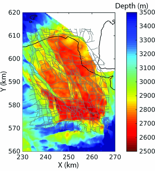
Fig. 1. Depth of top of Rotliegend and base of Zechstein of the Groningen gas field (Van Dalfsen et al., Reference Van Dalfsen, Doornenbal, Dortland and Gunnink2006). Faults at reservoir level (grey lines) are from Bourne et al. (Reference Bourne, Oates, van Elk and Doornhof2014).
The reservoir rock is sealed by a layer of Zechstein evaporites of varying thickness. The large seismic velocity contrast between the slower reservoir rock and faster evaporites significantly affects the waveforms (Kraaijpoel & Dost, Reference Kraaijpoel and Dost2013). Together with the irregular shapes of the Zechstein salt domes, this complicates the location of earthquakes by picking and inverting P- and S-wave arrival times.
Multiplet analysis
Data
The multiplet analysis was carried out for data of station WDB (53.2082°N, 6.7355°E), one of five borehole stations in the direct vicinity of the Groningen gas field (Fig. 2) of the pre-2015 network deployed by the Royal Netherlands Meteorological Institute (KNMI). The station consists of four three-component borehole geophones at depths varying from 47 to 197 m below sea level. The deepest geophone of station WDB, WDB4, suffering the least from surface noise, was selected for the multiplet analysis. We also analysed data of borehole stations ENM (53.4064°N, 6.4817°E) and SPY (53.4098°N, 6.7838°E) with a similar configuration to WDB, but, due to their closer proximity to the sea (Fig. 2), these stations had a lower signal-to-noise (S/N) ratio.
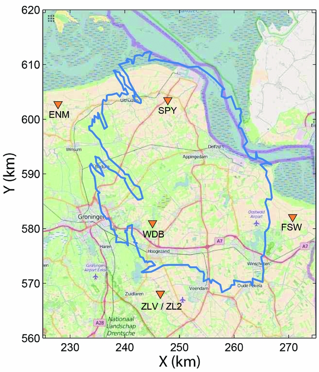
Fig. 2. Outline of the Groningen gas field (blue contour). Triangles indicate seismic stations of the pre-2015 network operated by the KNMI. Coordinates are given in kilometres within the Dutch National Triangulation Coordinates System (Rijksdriehoek). The background map is from www.openstreetmap.org.
The database of induced earthquakes, provided by the KNMI (http://rdsa.knmi.nl/dataportal), includes 426 events between January 2010 and 16 June 2014, the period of this study. Of these events, 212 are recorded by WDB4 and are used for the multiplet analysis. The locations in the KNMI catalogue are obtained using the method described in Lienert et al. (Reference Lienert, Berg and Frazer1986), with a depth fixed to 3 km. From 2015 onwards, depths are estimated using P-wave arrival time differences over the densified network (Spetzler & Dost, Reference Spetzler and Dost2016).
Method
The multiplet analysis used is described in detail in Dyer et al. (Reference Dyer, Schanz, Spillmann, Ladner and Häring2010). A summary of the approach is presented here. In the multiplet analysis, every recorded event is cross-correlated with every other event. The outcome is a symmetric cross-correlation matrix in which every element represents the normalised cross-correlation coefficient between two events. Seed events are then identified which define the multiplets. A seed event correlates with all other events in a multiplet at a level higher than a specified threshold, henceforth referred to as the seed level. Sometimes events already assigned to a multiplet are themselves seed events for another multiplet. In that case, the events belonging to this particular seed event are included in the multiplet that has the seed event in it. The threshold for correlating events to seed events may vary with the initial conditions, such as time window, noise level and frequency band. For each set of initial conditions several seed levels are examined. The criterion for choosing a seed level is whether the multiplets translate to spatial clusters. If the seed level is too low, the events in a multiplet will not be tightly clustered and it will be hard to distinguish multiplet groups (De Meersman et al., Reference De Meersman, Kendall and van der Baan2009). On the other hand, if the seed level is too high, there will be no multiplets to analyse. Seed events with the largest number of events obtain the highest status. If two or more seed events have multiplets of the same size then the seed event with the highest S/N ratio obtains the highest status. Finally, the original cross-correlation matrix is sorted according to the status of the multiplets.
The multiplet analysis was applied to both the N-component (horizontal north–south) and Z-component (vertical) of the deepest geophone of station WDB. S-wave arrivals are primarily detected on horizontal components, whereas P-wave arrivals are more prominent on the verticals. The time window of the records is determined by the duration of the wave field. The majority of the direct P-waves arrive at station WDB within 0–3 s after the established origin time of the earthquake. The coda waves no longer exceed the noise level after 50–60 s. As Schaff et al. (Reference Schaff, Bokelmann, Ellsworth, Zanzerkia, Waldhauser and Beroza2004) pointed out, correlation coefficients decrease with increasing window length. However, only taking into account the part containing most energy (2–25 s) did not produce neat clusters since the coda waves need to be correlated as well when events have nearby origins. Therefore the selected time window is set to 2–45 s.
Prior to this research, the optimum frequency band for the multiplet analysis of this dataset was unknown. In near-surface boreholes, induced seismicity is detected between about 1 and 30 Hz. The greatest similarity is found for the lower frequencies (1–10 Hz), because of the extent of the study area. For small study areas, higher frequencies are used (e.g. Moriya et al., Reference Moriya, Niitsuma and Baria2003). However, higher frequencies are more strongly affected by small-scale heterogeneities and scattering (Geller & Mueller, Reference Geller and Mueller1980), and a small disturbance in the ray path and/or source location can cause a large change in the high-frequency part of the signal. Three different frequency bands of 1–2 Hz, 1–4 Hz and 1–8 Hz were therefore investigated. The optimum frequency band turned out to be 1–8 Hz, because it takes into account the broadest frequency range of the signal, resulting in spatially tight clusters. Moreover, the largest number of clusters was obtained for this frequency band.
Results
We started the multiplet analysis with 212 events for WDB4. Events that did not have a cross-correlation coefficient >0.3 with any other event were removed to improve visualisation. After this operation, 113 and 145 events remained for the Z- and N-component, respectively. The seed level for the Z-component was set to 0.5, because it is the lowest seed level that produced the largest number of tightly spaced clusters. For the N-component the seed level was set at 0.6, because the overall cross-correlation coefficients are higher than for the Z-component. The cross-correlation matrices of the Z- and N-components of geophone WDB4, sorted after multiplet clustering, are shown in Figures 3 and 4, respectively. The red diagonal represents autocorrelation coefficients with a value of 1, and off-diagonal cross-correlation coefficients are generally small (<0.3). Multiplet analysis for the Z-component yielded one cluster of five events, two of four events and three of three events (Fig. 3). The N-component-based multiplet analysis yielded five clusters, where clusters 2–5 are identical to those obtained for the Z-component, and cluster 1 has four of the five events in common (Table 1). Cluster 6 is not identified on the N-component, possibly due to the higher seed level chosen. Figure 5 shows the traces of cluster 2 for the N-component to illustrate the waveform similarity within a multiplet. Waveform similarity in the part containing most of the energy (4–14 s) is not immediately apparent (Fig. 5b), validating our choice to cross-correlate the coda waves as well.

Fig. 3. Sorted cross-correlation matrix for 1–8 Hz: Z-component; geophone WDB4.

Fig. 4. Sorted cross-correlation matrix for 1–8 Hz: N-component; geophone WDB4.
Table 1. Event numbers in multiplets from the 1–8 Hz analysis for geophone WDB4. Event information of the event numbers is given in the Appendix. Seed events are bold.


Fig. 5. N-component traces of cluster 2 for time windows of (A) 2–45 s and (B) 4–14 s.
Thus, for the Z-component, out of all 212 analysed events recorded by geophone WDB4, 22 (10.4%) are clustered in six different multiplets. Figure 6 shows the locations of the clustered and non-clustered events, together with the coastline of Groningen, the main faults at the top of the Rotliegend sandstones and locations of seismic stations. Spatial clusters can be linked to faults in this way. Note that there are many tightly located events in Figure 6 that are nevertheless not part of a cluster. This suggests that many faults or fault segments are active, with possibly varying source mechanisms, resulting in greatly varying waveforms. Despite the similarity of their seismograms and the high cross-correlation values, the events in cluster 1 appear to be relatively widely distributed (within 13 km). Furthermore, for some of the events of this cluster, it is not possible to confidently pick the P- and S-wave arrival times at other stations than that used for the multiplet analysis (WDB4). The events of this cluster are therefore not relocated.
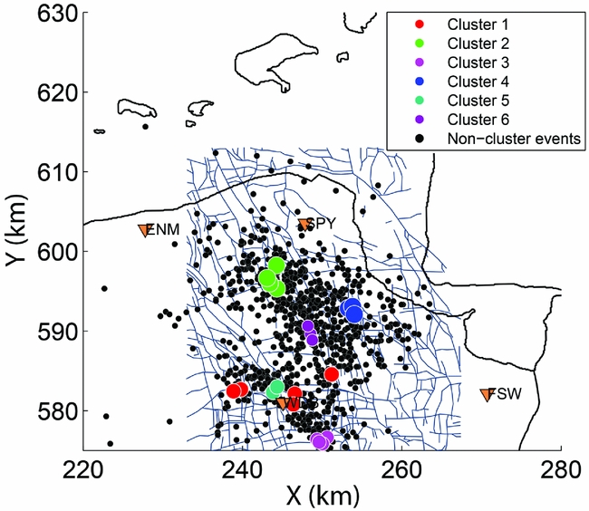
Fig. 6. Locations of Z-component-derived clusters, and non-clustered events, plotted in a map with the Groningen coastline. Sizes of the circles representing clustered events denote magnitudes. For reference, the locations of four borehole stations (orange triangles) are shown. Faults have been taken from Bourne et al. (Reference Bourne, Oates, van Elk and Doornhof2014).
We further quantified the similarity of the events within the different clusters by averaging the unique cross-correlation coefficients of each cluster. For a cluster with n events, there exist n(n − 1)/2 unique cross-correlations. The highest similarity is obtained for cluster 5 (0.72), which is close to station WDB that is used for the multiplet analysis (Fig. 6). Cluster 1, the cluster with the least dense confinement of events (Fig. 6), has the smallest similarity, together with cluster 6 (both have a similarity of 0.48). Cluster 2 (0.54), cluster 3 (0.62) and cluster 4 (0.65) show values in between.
Relocation
Method
The relocation method used in this study is an adapted version of the double-difference method of Waldhauser & Ellsworth (Reference Waldhauser and Ellsworth2000). It uses the travel time difference between the P- and S-waves to locate events relative to a master event. Schematically, the ray paths of P- or S-waves for events at epicentral distances larger than roughly 5 km are shown in Figure 7. The figure presents a simplification of the velocity structure of the Groningen area based on Duin et al. (Reference Duin, Doornenbal, Rijkers, Verbeek and Wong2006). The light-grey layer in Figure 7a with the two stars indicates the reservoir layer from the Rotliegend Group. The irregular layer on top of the reservoir is salt from the Zechstein Group. The Limburg Group directly below the reservoir has slightly higher velocities than the reservoir, whereas the underlying Lower Carboniferous Group (Dinantian) of compact limestones (darkest grey) is thought to have significantly higher seismic velocities. Vandenberghe et al. (Reference Vandenberghe, Poggiagliolmi and Watts1986) reported P-wave velocities of 4.9–5.6 km s−1 for karstified and 6.4 km s−1 for tight Dinantian limestones. When the distance between source and receiver is much larger than the source depth of 3 km, the first arriving P- and S-waves propagate as critically refracted head waves along this Lower Carboniferous Group or deeper strata. The P- and S-wave velocities of this refracting layer, 5.1 and 2.8 km s−1, respectively, are determined by linear regression of P- and S-wave onsets of an M = 2.4 2016 event that was recorded by many stations of the densified seismic network (Fig. 8). Seismic velocities are heterogeneous over the Groningen area (Duin et al., Reference Duin, Doornenbal, Rijkers, Verbeek and Wong2006), so Figure 7 is schematic.
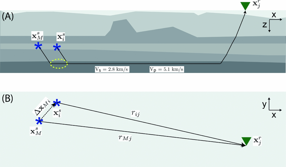
Fig. 7. Configuration for location of a source (blue star) in a cluster x s i with respect to a master source x s M and one of the receivers (green triangle): (A) section view, (B) map view. In (A) the blue stars are at the hypocentres, in (B) they correspond to the epicentres.
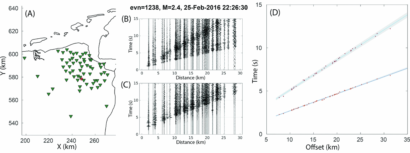
Fig. 8. Estimation of average P- and S-wave head-wave velocities over the Groningen area. (a) the configuration of the 2016 M = 2.4 Froombosch event (red circle) and the stations with borehole geophones recording the event (green triangles). (b) and (c) are the vertical and transverse component event gathers, respectively, frequency bandpass filtered between 1 and 25 Hz. (d) shows picks of first P-wave and S-wave onsets between 7 and 35 km offset, which are fitted with a straight line. Behind the picks, the 95 confidence areas are shown (grey zones). For the (refracted) P-wave the mean velocity is 5.06 km s−1 and the 95 confidence zone is bounded by a lower and upper velocity of 5.00 and 5.13 km s−1, respectively. For the (refracted) S-wave the mean velocity is 2.83 km s−1 and the 95 confidence zone is bounded by a lower and upper velocity of 2.79 and 2.87 km s−1, respectively.
All earthquakes are assumed to originate in the reservoir at 3 km depth. The blue stars in Figure 7 indicate the locations of an accurately determined master event, x s M , and the location of event i of the cluster x s i . Both events are detected at a receiver at location x r j , where j is the receiver index. Clustered events are located close to the master event, therefore the waves follow a similar path to the receiver and encounter a similar velocity structure. We want to relocate source x s i relative to x s M in the horizontal plane. The difference in horizontal distance between the source at x s i and master event at x s M as seen by the receiver at x r j reads
 $$\begin{equation*}
\Delta {r_{ij}} = {r_{ij}} - {r_{Mj}},
\end{equation*}$$
$$\begin{equation*}
\Delta {r_{ij}} = {r_{ij}} - {r_{Mj}},
\end{equation*}$$
where rij is the horizontal distance from x s i to x r j , which is computed by taking the Euclidean length ∥x s i − x j r ∥ for the horizontal coordinates. This distance can be expressed in terms of difference in travel time for the two sources in the first-arriving P-wave multiplied by the P-wave velocity of the refracting layer:
 $$\begin{equation}
\Delta {r_{ij}} = \left( {t_{ij}^P - t_{Mj}^P} \right){v^P},
\end{equation}$$
$$\begin{equation}
\Delta {r_{ij}} = \left( {t_{ij}^P - t_{Mj}^P} \right){v^P},
\end{equation}$$
and analogously for the first S-wave:
 $$\begin{equation}
\Delta {r_{ij}}\; = \;\left( {t_{ij}^S\; - \;t_{Mj}^S} \right){v^S}.
\end{equation}$$
$$\begin{equation}
\Delta {r_{ij}}\; = \;\left( {t_{ij}^S\; - \;t_{Mj}^S} \right){v^S}.
\end{equation}$$
The P- and S-wave velocities need only be known for the refracting layer in the small area Δx Mi indicated by the yellow ellipse in Figure 7a, and the velocities are assumed to be constant in this area. The travel time, t, is given by the difference between the arrival time, T, and the earthquake origin time, EOT, e.g. tP ij = Tij P − EOT. When eqn 1 is multiplied by vS on both sides, and eqn 2 by vP , and when the new eqn 1 is then subtracted from the new eqn 2, the dependence on the origin times vanishes:
 $$\begin{equation}
\Delta {r_{ij}}\; = \;\frac{{T_{ij}^S\; - \;T_{ij}^P\; - \;\left( {T_{Mj}^S\; - \;T_{Mj}^P} \right)}}{{\frac{1}{{{v^S}}}\; - \;\frac{1}{{{v^P}}}}} = \frac{{\Delta T_{ij}^{PS}\; - \;\Delta T_{Mj}^{PS}}}{{\frac{1}{{{v^S}}}\; - \;\frac{1}{{{v^P}}}}}.
\end{equation}$$
$$\begin{equation}
\Delta {r_{ij}}\; = \;\frac{{T_{ij}^S\; - \;T_{ij}^P\; - \;\left( {T_{Mj}^S\; - \;T_{Mj}^P} \right)}}{{\frac{1}{{{v^S}}}\; - \;\frac{1}{{{v^P}}}}} = \frac{{\Delta T_{ij}^{PS}\; - \;\Delta T_{Mj}^{PS}}}{{\frac{1}{{{v^S}}}\; - \;\frac{1}{{{v^P}}}}}.
\end{equation}$$
Expressing source location x s i as function of the master event location, x s i = x M s + Δx Mi = (xs i + ΔxMi , ys i + ΔyMi ), eqn 3 can be rewritten as
 $$\begin{equation}
\begin{array}{l}
\left( \parallel {\rm{x}}_j^r\; - \;{\rm{x}}_M^s\; - \;\Delta {{\rm{x}}_{Mi}}\parallel \; - \;\parallel {\rm{x}}_j^r\; - \;{\rm{x}}_M^s\parallel \right)\left( {\frac{1}{{{v^S}}}\; - \;\frac{1}{{{v^P}}}} \right)\\
\qquad = \;\Delta T_{ij}^{PS}\; - \;\Delta T_{Mj}^{PS},\end{array}
\end{equation}$$
$$\begin{equation}
\begin{array}{l}
\left( \parallel {\rm{x}}_j^r\; - \;{\rm{x}}_M^s\; - \;\Delta {{\rm{x}}_{Mi}}\parallel \; - \;\parallel {\rm{x}}_j^r\; - \;{\rm{x}}_M^s\parallel \right)\left( {\frac{1}{{{v^S}}}\; - \;\frac{1}{{{v^P}}}} \right)\\
\qquad = \;\Delta T_{ij}^{PS}\; - \;\Delta T_{Mj}^{PS},\end{array}
\end{equation}$$
where the right-hand side is the difference in arrival time between the P- and S-wave of source i recorded by receiver j minus the same difference but then for the master event. To compute the relative horizontal location of source x s i with respect to x s M , eqn 4 must be solved for at least two receivers to find the two unknowns Δx Mi and ΔyMi .
Using this approach with relative locations with respect to a nearby master event, location errors caused by a simplification of the 3D velocity structure (Van Dalfsen et al., Reference Van Dalfsen, Doornenbal, Dortland and Gunnink2006) by a 1D model (Kraaijpoel & Dost, Reference Kraaijpoel and Dost2013) are largely circumvented. Furthermore, the dependence on origin time is eliminated, and erroneous arrival time picks for events with a low S/N ratio are reduced by using cross-correlations. For each cluster of events, we first select a time window around the first P-wave arrival. Then we estimate the difference in P-wave arrival time between the master source and cluster sources by cross-correlating the selected time window, yielding
 $$\begin{equation}
\Delta T_{ij}^P\; = \;EO{T_i}\; + \;t_{ij}^P\; - \;\left( {EO{T_M}\; + \;t_{Mj}^P} \right),
\end{equation}$$
$$\begin{equation}
\Delta T_{ij}^P\; = \;EO{T_i}\; + \;t_{ij}^P\; - \;\left( {EO{T_M}\; + \;t_{Mj}^P} \right),
\end{equation}$$
where EOTi is the initial estimate of EOT for source i. For sources for which the P-wave arrivals are not sufficiently similar, we use kurtosis with its positive derivative (Langet et al., Reference Langet, Maggi, Michelini and Brenguier2014) to obtain time series that are peaked at the P-wave onsets. These peaks are highly similar for the different events and thus lead to accurate time differences after cross-correlation. We also estimate relative S-wave arrival times with cross-correlation (or the cross-correlation of the positive derivative of kurtosis, if required), yielding an equivalent expression for S-waves:
 $$\begin{equation}
\Delta T_{ij}^S\; = \;EO{T_i}\; + \;t_{ij}^S\; - \;\left( {EO{T_M}\; + \;t_{Mj}^S} \right).
\end{equation}$$
$$\begin{equation}
\Delta T_{ij}^S\; = \;EO{T_i}\; + \;t_{ij}^S\; - \;\left( {EO{T_M}\; + \;t_{Mj}^S} \right).
\end{equation}$$
The EOTs cancel when eqn 5 is subtracted from eqn 6, and the S–P arrival time difference is obtained (right-hand side of eqn 4).
To find the relative locations of sources in the cluster with respect to the master event we do a grid search for eqn 4. We define a grid around the master event for which we forward-model the left-hand side of eqn 4. So for each potential relative location Δx Mi , the misfit R is computed between the estimated and recorded S–P arrival time difference:
 {\fontsize{7}{9}\selectfont{$$\begin{equation}
R\left( {\Delta {{\rm{x}}_{Mi}}} \right)\; = \;\sqrt {\mathop \sum \limits_{j\; = \;1}^n {{\left\{ {{{\left( {\Delta T_{ij}^{PS}\; - \;T_{Mj}^{PS}} \right)}^{obs}}\; - \;{{\left( {\Delta T_{ij}^{PS}\left( {\Delta {{\rm{x}}_{Mi}}} \right)\; - \;\Delta T_{Mj}^{PS}} \right)}^{mod}}} \right\}}^2}/n} ,
\end{equation}$$}}
{\fontsize{7}{9}\selectfont{$$\begin{equation}
R\left( {\Delta {{\rm{x}}_{Mi}}} \right)\; = \;\sqrt {\mathop \sum \limits_{j\; = \;1}^n {{\left\{ {{{\left( {\Delta T_{ij}^{PS}\; - \;T_{Mj}^{PS}} \right)}^{obs}}\; - \;{{\left( {\Delta T_{ij}^{PS}\left( {\Delta {{\rm{x}}_{Mi}}} \right)\; - \;\Delta T_{Mj}^{PS}} \right)}^{mod}}} \right\}}^2}/n} ,
\end{equation}$$}}
for n receivers where both earthquake i and master event M are observed with sufficient S/N ratio.
Since a homogeneous velocity field is used, no local minima exist in this misfit function. The trial location with the smallest misfit is assigned to be the relocated source location.
Results
For relocation we use master events of which the locations are known much more accurately than those of the pre-2015 monitoring network. These master events were recorded by a network that by the end of 2015 consisted of more than 60 boreholes in and around the Groningen gas field (https://www.knmi.nl/nederland-nu/seismologie/stations). The cluster events are recorded by at most five borehole stations in the region (see Fig. 2). The S–P arrival time differences are determined from the bottom geophones in the boreholes.
For cluster 2 we used event 1147 (see Appendix) to serve as master event. Boreholes SPY, ENM and WDB were used for the intra-cluster relocations. The result of the relocation is shown in Figure 9a. The KNMI estimated that one event (755) in cluster 2 was located significantly farther away from the other events. Our results show, however, that all relocated events plot on a small area close to one or two faults. The misfit (eqn 7) prior to and after relocation is given in Table 2. Event 755 shows the largest misfit reduction, of almost a factor 8.
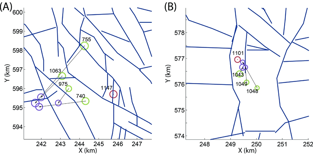
Fig. 9. Relocations for (A) cluster 2 and (B) cluster 3. Green circles represent locations estimated by the KNMI, purple circles the new locations and red circles denote locations of the master events. The size of the circles scales with the magnitude. The black arrows denote relocation vectors, and the blue lines denote identified faults taken from Bourne et al. (Reference Bourne, Oates, van Elk and Doornhof2014). Additional information on the numbered events can be found in the Appendix.
Table 2. For each relocated event the root-mean-square error (RMSE) prior to and after relocation (eqn 7) is tabulated.

Event 1101 was selected as a master event for cluster 3. Only three of the four events of this cluster could be relocated, because the S/N ratio of one event was too low to estimate the S–P arrival time difference. Originally, the remaining events were already located relatively close together, but the relocation method with data from boreholes WDB, ZLV and FSW has brought the events even closer together and closer to the master event (Fig. 9b).
Data from boreholes WDB, ZLV and FSW were used to relocate the events of cluster 4 with master event 1142. The new locations are more tightly clustered at two nearby faults (Fig. 10a).
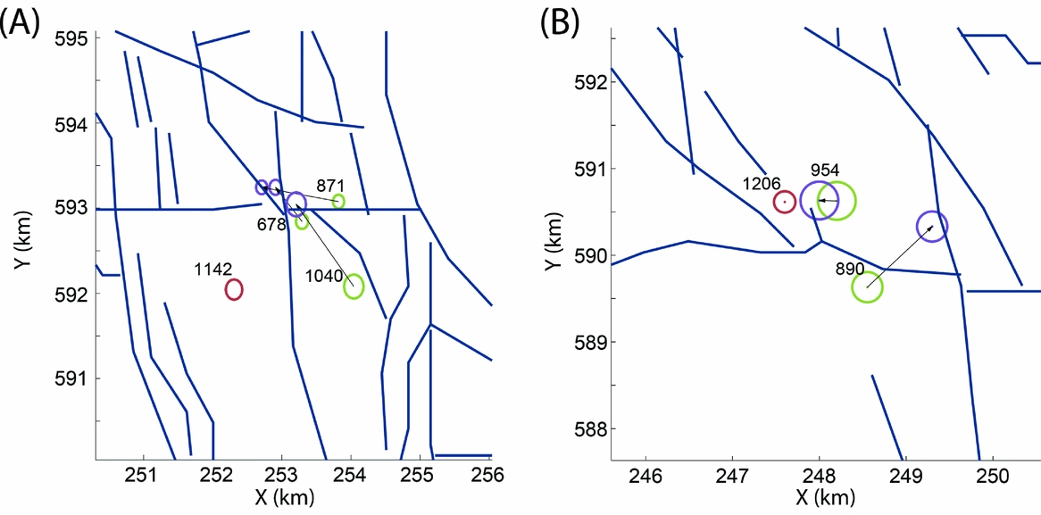
Fig. 10. Relocations for (A) cluster 4 and (B) cluster 6. Green circles represent locations estimated by the KNMI, purple circles the new locations and red circles denote locations of the master events. The black arrows denote relocation vectors and the blue lines denote identified faults taken from Bourne et al. (Reference Bourne, Oates, van Elk and Doornhof2014). Additional information on the numbered events can be found in the Appendix.
It was not possible to improve the relative locations of the events of cluster 5, because the S/N ratio at SPY and FSW was too low to determine the differential arrival times. The three remaining stations, ENM, WDB and ZLV, are nearly aligned in a NNW–SSE direction. Their data do not constrain the locations in E–W direction very well. The event locations could be shifted in this direction and still give a good fit to the data.
Cluster 6 comprises two events of relatively high magnitude (M = 2.4 and 3.0 for events 890 and 954, respectively) and one event of low magnitude (M = 0.9, event 972). The S/N ratio of this last event is too low to identify its P- and S-arrivals at borehole locations WDB, FSW and ENM. The remaining two events are relocated with respect to event number 1206. The events are relocated to two parallel faults as shown in Figure 10b.
The events in clusters 2, 3 and 6 are relocated with respect to nearby and high S/N-ratio events from the densified array. Only for cluster 4 could a master event be found that is also formally a seed event and hence part of the cluster. Since the multiplet analysis did not include post-2014 events, this master event was not part of cluster 4 in the first section of this paper.
Discussion and conclusion
Up to now, most multiplet analyses have been applied to identify clusters of tectonic events (e.g. Myhill et al., Reference Myhill, McKenzie and Priestley2011; Lambotte et al., Reference Lambotte, Lyon-Caen, Bernard, Deschamps, Nercessian, Pacciani, Bourouis, Drilleau and Adamova2014) or induced events recorded at deep boreholes (e.g. Michelet & Toksöz, Reference Michelet and Toksöz2007; De Meersman et al., Reference De Meersman, Kendall and van der Baan2009). The multiplet analysis presented here shows that it is also feasible to identify clusters of induced events in the Groningen gas field, an area with a diameter of roughly 30 km. Approximately 10% of the events recorded at station WDB between 2010 and mid-2014 could be assigned to one of six clusters of events when a relatively broad frequency range, 1–8 Hz, of the data is used. With a seed level of 0.5–0.6 the correlation between events is smaller than for induced events recorded at deep boreholes near the seismicity (e.g. Arrowsmith & Eisner, Reference Arrowsmith and Eisner2006). This indicates that the events are probably not always located on the same faults or that they have slightly different source mechanisms. In our relocation, only the events in cluster 3 are confined within a few hundred metres on the same fault (Fig. 9b).
Approximately 90% of the analysed events are not part of a cluster, despite the low threshold chosen (0.5) and despite small distances between events. This suggests that, even at close range, many different faults and/or fault segments are active in the Groningen field, with likely also a spread in focal mechanisms.
The cluster events recorded by the pre-2015 seismic network are relocated using master events from 2015 to March 2016 that are localised by a much denser seismic network in the Groningen area. The master events are located with only upgoing P-waves, for which velocities are well known from 3D seismics and numerous borehole logs. The relocation method is based on S–P arrival time differences of cluster events with respect to master events. Using cross-correlation, the S–P arrival time differences are determined at a minimum of two stations to allow relocation in the horizontal plane. With the ray paths of the P- and S-waves of the cluster events and the master event being very similar, the relocated events are found to be more tightly clustered than the original locations and are located close to existing faults (Figs 9, 10). The relocation yielded reductions in root-mean-square error ranging from a small fraction to a factor of 10.
The largest error in the location is thought to be caused by errors in the velocity model. The pre-2015 KNMI locations are susceptible to velocity uncertainty over large distances between source and receivers. The relocation is sensitive primarily to velocity uncertainty in a region around a source cluster. Consequently, less location error is accrued due to velocity uncertainty for the relocation than for the original location, which is sensitive to velocities on the entire source–receiver path. However, the relocation will only yield better absolute locations when there is little location uncertainty for the master event.
The similarity of the clustered events was found to be relatively low for the Groningen setting. The average similarity within the clusters was 0.58. As a consequence, we could not fully rely on cross-correlations of the original waveforms to obtain travel time differences. We therefore applied kurtosis to some of the waveforms to obtain more accurate measurements of time differences. Moreover, due to insufficient S/N ratio of the most energetic P-wave and/or S-wave package on some of the stations, we could not apply relocation to events in clusters 1 and 5 and a few events in other clusters.
We restricted ourselves to relocating the identified clustered events. The relocation approach taken, however, could be expanded to all pre-2015 events that are in the vicinity of master events located with the densified network, as our results suggest that this relocation method improves the event locations.
Acknowledgements
We would like to thank Bernard Dost for advice and Gert-Jan van den Hazel and Jordi Domingo Ballesta for KNMI data preparation. We would also like to thank the reviewers Ben Dyer and Dirk Kraaijpoel, and the advisors Hirokazu Moriya, Allan Rubin and Ólafur Gudmundsson, for suggestions that helped to improve the manuscript.
Appendix
Table A1. Event information of cluster and master events (source: http://rdsa.knmi.nl/dataportal).


 Open access