


1 Introduction
The instrumental variable (IV) approach is a widely used empirical method in the social sciences, including political science, for establishing causal relationships. It is often used when selection on observables is implausible, experimentation is infeasible or unethical, and rule-based assignments that allow for sharp regression-discontinuity (RD) designs are unavailable. In recent years, there have been a growing number of articles published in top political science journals, such as the American Political Science Review (APSR), American Journal of Political Science (AJPS), and The Journal of Politics (JOP), that use IV as a primary causal identification strategy (Figure 1). This trend can be traced back to the publication of Mostly Harmless Econometrics (Angrist and Pischke Reference Angrist and Pischke2009), which popularized the modern interpretation of IV designs, and Sovey and Green (Reference Sovey and Green2011), which clarifies the assumptions required by an IV design and provides a useful checklist for political scientists.
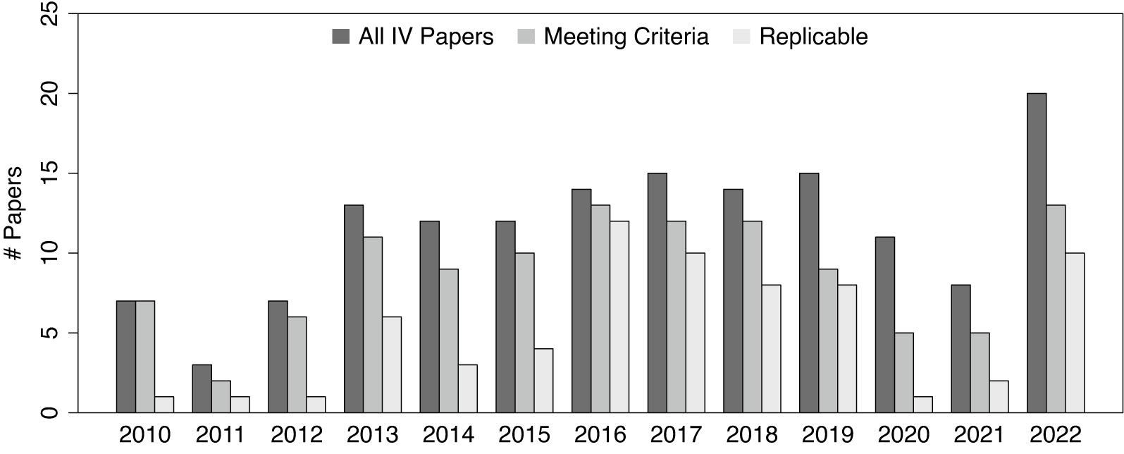
Figure 1 IV studies published in the APSR, AJPS, and JOP. Our criteria rule out IV models appearing in the Supplementary Material only, in dynamic panel settings, with multiple endogenous variables, and with nonlinear link functions. Non-replicability is primarily due to a lack of data and/or coding errors.
Despite its popularity, the IV approach has faced scrutiny from researchers who note that two-stage least-squares (2SLS) estimates are often much larger in magnitude than “naïve” ordinary-least-squares (OLS) estimates, even when the main concern with the latter is upward omitted-variables bias.Footnote 1 Others have raised concerns about the validity of the commonly used inferential method for 2SLS estimation (e.g., Lee et al. Reference Lee, McCrary, Moreira and Porter2022; Young Reference Young2022).
These observations motivate our systematic examination of the use of IVs in the empirical political science literature. We set out to replicate all studies published in the APSR, AJPS, and JOP during the past 13 years (2010–2022) that use an IV design with a single endogenous variable as one of the main identification strategies.Footnote 2 Out of 114 articles meeting this criterion, 71 have complete replication materials online, which is concerning in itself. We successfully replicated at least one primary IV result in 67 out of the remaining 71 articles. Among the 67 articles, three articles feature two distinct IV designs, each yielding two separate replicable IV results.
Using data from these 70 IV designs, we conduct a programmatic replication exercise and find three troubling patterns. First, a significant number of IV designs in political science overestimate the first-stage partial F-statistic by failing to adjust standard errors (SEs) for factors such as heteroskedasticity, serial correlation, or clustering structure. Using the effective F-statistic (Olea and Pflueger Reference Olea and Pflueger2013), we find that at least 11% of the published IV studies rely on what econometricians call “weak instruments,” the consequences of which have been well documented in the literature. See Andrews, Stock, and Sun (Reference Andrews, Stock and Sun2019) for a comprehensive review.
Second, obtaining valid statistical inferences for IV estimates remains challenging. Almost all studies we have replicated rely on t-tests for the 2SLS estimates based on analytic SEs and traditional critical values (such as 1.96 for statistical significance at the 5% level). Using analytic SEs, IV estimates are already shown to be much more imprecise than OLS estimates. When employing bootstrapping procedures, the AR test, or the $tF$
procedure—an F-statistic-dependent t-test (Lee et al. Reference Lee, McCrary, Moreira and Porter2022)—for hypothesis testing, we find that 17%–35% of the designs cannot reject the null hypothesis of no effect at the 5% level. In contrast, only 10% of studies based on originally reported SEs or p-values fail to reject the null hypothesis. This discrepancy suggests that many studies may have underestimated the uncertainties associated with their 2SLS estimates.
$tF$
procedure—an F-statistic-dependent t-test (Lee et al. Reference Lee, McCrary, Moreira and Porter2022)—for hypothesis testing, we find that 17%–35% of the designs cannot reject the null hypothesis of no effect at the 5% level. In contrast, only 10% of studies based on originally reported SEs or p-values fail to reject the null hypothesis. This discrepancy suggests that many studies may have underestimated the uncertainties associated with their 2SLS estimates.
What is even more concerning is that an IV approach can produce larger biases than OLS when a weak first-stage amplifies biases due to failures of IVs’ unconfoundedness or exclusion restrictions. We observe that in 68 out of the 70 designs (97%), the 2SLS estimates have a larger magnitude than the naïve OLS estimates obtained from regressing the outcome on potentially endogenous treatment variables and covariates; 24 of these (34%) are at least five times larger. This starkly contrasts with the common rationale for using IV, which is to mitigate the upward bias in treatment effect estimates from OLS. Moreover, we find that the ratio between the magnitudes of the 2SLS and OLS estimates is strongly negatively correlated with the strength of the first stage among studies that use nonexperimental instruments, and the relationship is almost nonexistent among experimental studies. While factors such as heterogeneous treatment effects and measurement error might be at play, we contend that this phenomenon primarily stems from a combination of weak instruments and the failure of unconfoundedness or the exclusion restriction. Intuitively, because the 2SLS estimator is a ratio, an inflated numerator from invalid instruments paired with a small denominator due to a weak first stage leads to a disproportionately large estimate. Publication bias and selective reporting exacerbate this issue.
What do these findings imply for IV studies in political science? First, the traditional F-tests for IV strength, particularly when using classic analytic SEs, often mask the presence of weak instruments. Second, when operating with these weak instruments, particularly in overidentified scenarios, traditional t-tests do not adequately represent the considerable uncertainty surrounding the 2SLS estimates, paving the way for selective reporting and publication bias. Last but not least, many 2SLS estimates likely bear significant biases due to violations of unconfoundedness or the exclusion restriction, and a weak first-stage further exacerbates these biases. While we cannot pinpoint exactly which estimates are problematic, these issues seem to be pervasive across observational IV studies. The objective of this paper, however, is not to discredit existing IV research or dissuade scholars from using IVs. On the contrary, our intent is to caution researchers against the pitfalls of ad hoc justifications for IVs in observational research and provide constructive recommendations for future practices. These suggestions include accurately quantifying the strength of instruments, conducting valid inference for IV estimates, as well as implementing additional validation exercises, such as placebo tests, to bolster the identifying assumptions.
Our work builds on a growing literature evaluating IV strategies in social sciences and offering methods to improve empirical practice. Notable studies include Young (Reference Young2022), which finds IV estimates to be more sensitive to outliers and conventional t-tests to understate uncertainties; Jiang (Reference Jiang2017), which observes larger IV estimates in finance journals and attributed this to exclusion restriction violations and weak instruments; Mellon (Reference Mellon2023), which emphasizes the vulnerability of weather instruments; Dieterle and Snell (Reference Dieterle and Snell2016), which develops a quadratic overidentification test and discovers significant nonlinearities in the first stage regression; Felton and Stewart (Reference Felton and Stewart2022), which finds unstated assumptions and a lack of weak-instrument robust tests in top sociology journals; and Cinelli and Hazlett (Reference Cinelli and Hazlett2022), which proposes a sensitivity analysis for IV designs in an omitted variable bias framework. This study is the first comprehensive replication effort focusing on IV designs in political science and uses data to shed light on the consequences of a weak first-stage interacting with failures of unconfoundedness or the exclusion restriction.
2 Theoretical Refresher
In this section, we offer a brief overview of the IV approach, including the setup, the key assumptions, and the 2SLS estimator. We then discuss potential pitfalls and survey several inferential methods. To cover the vast majority of IV studies in political science, we adopt a traditional constant treatment effect approach, which imposes a set of parametric assumptions. For example, of our replication sample, 51 designs (73%) employ continuous treatment variables, and 49 (70%) use continuous IVs. Most of these studies make no reference to treatment effect heterogeneity and are ill-suited for the local average treatment effect framework (Angrist, Imbens, and Rubin Reference Angrist, Imbens and Rubin1996).
Apart from the canonical use of IVs in addressing noncompliance in experimental studies, we observe that in the majority of the articles we review, researchers use IVs to establish causality between a single treatment variable d and an outcome variable y in observational settings. The basic idea of this approach is to use a vector of instruments z to isolate “exogenous” variation in d (i.e., the variation in d that is not related to potential confounders) and estimate its causal effect on y. For simplicity, we choose not to include any additional exogenous covariates in our discussion. This is without loss of generality because, by the Frisch–Waugh–Lovell theorem, we can remove these variables by performing a regression of y, d, and each component of z on the controls and then proceeding with our analysis using the residuals instead.
2.1 Identification and Estimation
Imposing a set of parametric assumptions, we define a system of simultaneous equations:
 $$ \begin{align} \text{Structural equation:}\quad y =&\ \tau_{0} + \tau d + \varepsilon, \end{align} $$
 $$ \begin{align}\ \text{First-stage equation:}\quad d =&\ \pi_0 + \pi' z + \nu, \end{align} $$
in which y is the outcome variable; d is a scalar treatment variable; z is a vector of instruments for d; and $\tau $
captures the (constant) treatment effect and is the key quantity of interest. The error terms
$\tau $
captures the (constant) treatment effect and is the key quantity of interest. The error terms $\varepsilon $
and
$\varepsilon $
and $\nu $
may be correlated. The endogeneity problem for
$\nu $
may be correlated. The endogeneity problem for $\tau $
in Equation (2.1) arises when d and
$\tau $
in Equation (2.1) arises when d and $\varepsilon $
are correlated, which renders
$\varepsilon $
are correlated, which renders $\hat \tau _{OLS}$
from a naïve OLS regression of y on d inconsistent. This may be due to several reasons: (1) unmeasured omitted variables correlated with both y and d, (2) measurement error in d, or (3) simultaneity or reverse causality, which means y may also affect d. Substituting d in Equation (2.1) using Equation (2.2), we have the reduced form equation:
$\hat \tau _{OLS}$
from a naïve OLS regression of y on d inconsistent. This may be due to several reasons: (1) unmeasured omitted variables correlated with both y and d, (2) measurement error in d, or (3) simultaneity or reverse causality, which means y may also affect d. Substituting d in Equation (2.1) using Equation (2.2), we have the reduced form equation:
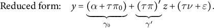 $$ \begin{align} \text{Reduced form:}\quad y = \underbrace{(\alpha + \tau \pi_0)}_{\gamma_0} + \underbrace{(\tau \pi)^{\prime}}_{\gamma'} z + (\tau\nu + \varepsilon). \end{align} $$
Substitution establishes that $\gamma = \tau \pi $
, rearranging yields
$\gamma = \tau \pi $
, rearranging yields $\tau = \frac {\gamma }{\pi }$
(assuming a single instrument, but the intuition carries over to cases with multiple instruments). The IV estimate, therefore, is the ratio of the reduced-form and first-stage coefficients. To identify
$\tau = \frac {\gamma }{\pi }$
(assuming a single instrument, but the intuition carries over to cases with multiple instruments). The IV estimate, therefore, is the ratio of the reduced-form and first-stage coefficients. To identify $\tau $
, we make the following assumptions (Greene Reference Greene2003, Chapter 12).
$\tau $
, we make the following assumptions (Greene Reference Greene2003, Chapter 12).
Assumption 1 Relevance $\pi \neq 0$
. This assumption requires that the IVs can predict the treatment variable, and is therefore equivalently stated as
$\pi \neq 0$
. This assumption requires that the IVs can predict the treatment variable, and is therefore equivalently stated as ![]() .
.
Assumption 2 Exogeneity: unconfoundedness and the exclusion restriction $\mathbb {E}[\varepsilon ] =0$
and
$\mathbb {E}[\varepsilon ] =0$
and $\text {Cov}(z, \varepsilon ) = 0$
. This assumption is satisfied when unconfoundedness (random or quasi-random assignment of z) and the exclusion restriction (no direct effect of z on y beyond d) are met.
$\text {Cov}(z, \varepsilon ) = 0$
. This assumption is satisfied when unconfoundedness (random or quasi-random assignment of z) and the exclusion restriction (no direct effect of z on y beyond d) are met.
Conceptually, unconfoundedness and the exclusion restriction are two distinct assumptions and should be justified separately in a research design. However, because violations of either assumption lead to the failure of the 2SLS moment condition, $\mathbb {E}[z\varepsilon ] = 0$
, and produce observationally equivalent outcomes, we consider both to be integral components of Assumption 2.
$\mathbb {E}[z\varepsilon ] = 0$
, and produce observationally equivalent outcomes, we consider both to be integral components of Assumption 2.
Under Assumptions 1 and 2, the 2SLS estimator is shown to be consistent for the structural parameter $\tau $
. Consider a sample of N observations. We can write
$\tau $
. Consider a sample of N observations. We can write $\mathbf {d} = (d_1, d_2, \ldots , d_N)'$
and
$\mathbf {d} = (d_1, d_2, \ldots , d_N)'$
and $\mathbf {y}= (y_1, y_2, \ldots , y_N)'$
as
$\mathbf {y}= (y_1, y_2, \ldots , y_N)'$
as $(N\times 1)$
vectors of the treatment and outcome data, and
$(N\times 1)$
vectors of the treatment and outcome data, and $\mathbf {z}= (z_1, z_2, \ldots , z_N)'$
as an
$\mathbf {z}= (z_1, z_2, \ldots , z_N)'$
as an $(N\times p_z)$
matrix of instruments in which
$(N\times p_z)$
matrix of instruments in which $p_z$
is the number of instruments. The 2SLS estimator is written as follows:
$p_z$
is the number of instruments. The 2SLS estimator is written as follows:
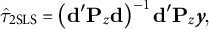 $$ \begin{align} \hat\tau_{\text{2SLS}} = \left({\mathbf{d}' \mathbf{P}_{z} \mathbf{d}} \right)^{-1} \mathbf{d}' \mathbf{P}_{z} \boldsymbol{y}, \end{align} $$
in which $\mathbf {P}_{z} = \mathbf {z} \left ({\mathbf {z}' \mathbf {z}} \right )^{-1} \mathbf {z}'$
is the hat-maker matrix from the first stage which projects the endogenous treatment variable
$\mathbf {P}_{z} = \mathbf {z} \left ({\mathbf {z}' \mathbf {z}} \right )^{-1} \mathbf {z}'$
is the hat-maker matrix from the first stage which projects the endogenous treatment variable $\mathbf {d}$
into the column space of
$\mathbf {d}$
into the column space of $\mathbf {z}$
, thereby in expectation preserving only the exogenous variation in
$\mathbf {z}$
, thereby in expectation preserving only the exogenous variation in $\mathbf {d}$
that is uncorrelated with
$\mathbf {d}$
that is uncorrelated with $\varepsilon $
. This formula permits the use of multiple instruments, in which case the model is said to be “overidentified.” The 2SLS estimator belongs to a class of generalized method of moments (GMM) estimators taking advantage of the moment condition
$\varepsilon $
. This formula permits the use of multiple instruments, in which case the model is said to be “overidentified.” The 2SLS estimator belongs to a class of generalized method of moments (GMM) estimators taking advantage of the moment condition $\mathbb {E}[z\varepsilon ] =0$
, including the two-step GMM (Hansen Reference Hansen1982) and limited information maximum likelihood estimators (Anderson, Kunitomo, and Sawa Reference Anderson, Kunitomo and Sawa1982). We use the 2SLS estimator throughout the replication exercise because of its simplicity and because every single paper in our replication sample uses it in at least one specification.
$\mathbb {E}[z\varepsilon ] =0$
, including the two-step GMM (Hansen Reference Hansen1982) and limited information maximum likelihood estimators (Anderson, Kunitomo, and Sawa Reference Anderson, Kunitomo and Sawa1982). We use the 2SLS estimator throughout the replication exercise because of its simplicity and because every single paper in our replication sample uses it in at least one specification.
When the model is exactly identified, that is, the number of treatment variables equals the number of instruments, the 2SLS estimator can be simplified as the IV estimator: $\hat {\tau }_{\text {2SLS}} = \hat {\tau }_{\text {IV}} = \left ({\mathbf {z}'\mathbf {d}} \right )^{-1} \mathbf {z}'\mathbf {y}$
. In the case of one instrument and one treatment, the 2SLS estimator can also be written as a ratio of two sample covariances:
$\hat {\tau }_{\text {2SLS}} = \hat {\tau }_{\text {IV}} = \left ({\mathbf {z}'\mathbf {d}} \right )^{-1} \mathbf {z}'\mathbf {y}$
. In the case of one instrument and one treatment, the 2SLS estimator can also be written as a ratio of two sample covariances: $\hat {\tau }_{2SLS} = \hat {\tau }_{IV} = \frac {\hat \gamma }{\hat \pi } = \frac {\widehat {\mathrm {Cov}}(y, z)}{\widehat {\mathrm {Cov}}(d, z)}$
, which illustrates that the 2SLS estimator is a ratio between reduced-form and first-stage coefficients in this special case. This further simplifies to a ratio of the differences in means when z is binary, which is called a Wald estimator.
$\hat {\tau }_{2SLS} = \hat {\tau }_{IV} = \frac {\hat \gamma }{\hat \pi } = \frac {\widehat {\mathrm {Cov}}(y, z)}{\widehat {\mathrm {Cov}}(d, z)}$
, which illustrates that the 2SLS estimator is a ratio between reduced-form and first-stage coefficients in this special case. This further simplifies to a ratio of the differences in means when z is binary, which is called a Wald estimator.
2.2 Potential Pitfalls in Implementing an IV Strategy
The challenges with 2SLS estimation and inference are mostly due to violations of Assumptions 1 and 2. Such violations can result in (1) significant uncertainties around 2SLS estimates and size distortion for t-tests due to weak instruments even when the exogeneity assumption is satisfied and (2) potentially larger biases in 2SLS estimates compared to OLS estimates when the exogeneity assumption is violated.
2.2.1 Inferential Problem Due to Weak Instruments
Since the IV coefficient is a ratio, the weak instrument problem is a “divide-by-zero” problem, which arises when $\text {Cov}(z, d) \approx 0$
(i.e., when the relevance assumption is violated). The instability of ratio estimators like
$\text {Cov}(z, d) \approx 0$
(i.e., when the relevance assumption is violated). The instability of ratio estimators like $\widehat {\tau }_{\text {2SLS}}$
when the denominator is approximately zero has been extensively studied going back to Fieller (Reference Fieller1954). The conventional wisdom in the past two decades has been that the first-stage partial F-statistic needs to be bigger than 10, and it should be clearly reported (Staiger and Stock Reference Staiger and Stock1997). The cutoff, as a rule of thumb, is chosen based on simulation results to meet two criteria under i.i.d. errors: (1) in the worst case, the bias of the 2SLS estimator does not exceed 10% of the bias of the OLS estimator and (2) a t-test based on the 2SLS estimator with a size of 5% does not lead to size over 15%. These problems are further exacerbated in settings where units belong to clusters with strong within-cluster correlation, where a small number of observations or clusters may heavily influence estimated results (Young Reference Young2022). Recently, however, Angrist and Kolesár (Reference Angrist and Kolesár2023) argue that the conventional inference strategies are reliable in just-identified settings with independent errors. The weak instrument issue is indeed most concerning in heavily overidentified scenarios.
$\widehat {\tau }_{\text {2SLS}}$
when the denominator is approximately zero has been extensively studied going back to Fieller (Reference Fieller1954). The conventional wisdom in the past two decades has been that the first-stage partial F-statistic needs to be bigger than 10, and it should be clearly reported (Staiger and Stock Reference Staiger and Stock1997). The cutoff, as a rule of thumb, is chosen based on simulation results to meet two criteria under i.i.d. errors: (1) in the worst case, the bias of the 2SLS estimator does not exceed 10% of the bias of the OLS estimator and (2) a t-test based on the 2SLS estimator with a size of 5% does not lead to size over 15%. These problems are further exacerbated in settings where units belong to clusters with strong within-cluster correlation, where a small number of observations or clusters may heavily influence estimated results (Young Reference Young2022). Recently, however, Angrist and Kolesár (Reference Angrist and Kolesár2023) argue that the conventional inference strategies are reliable in just-identified settings with independent errors. The weak instrument issue is indeed most concerning in heavily overidentified scenarios.
The literature has discussed at least three issues caused by weak instruments when the exogeneity assumption is satisfied. First, under i.i.d. errors, a weak first stage exacerbates the finite-sample bias of the 2SLS estimator toward the inconsistent OLS estimator, thereby reproducing the endogeneity problem that an IV design was meant to solve (Staiger and Stock Reference Staiger and Stock1997). Additionally, when the first stage is weak, the 2SLS estimator may not have a mean; its median is centered around the OLS coefficient (Hirano and Porter Reference Hirano and Porter2015). Second, the 2SLS estimates become very imprecise. To illustrate, a commonly used variance estimator for $\hat {\tau }_{IV}$
is
$\hat {\tau }_{IV}$
is $\hat {\mathbb {V}}(\hat {\tau }_{IV}) \approx \hat {\sigma }^2/(\sum _{i=1}^N (d_i - \overline {d})^2 R_{dz}^2) = \hat {\mathbb {V}}(\hat {\tau }_{OLS}) /R_{dz}^2$
, in which
$\hat {\mathbb {V}}(\hat {\tau }_{IV}) \approx \hat {\sigma }^2/(\sum _{i=1}^N (d_i - \overline {d})^2 R_{dz}^2) = \hat {\mathbb {V}}(\hat {\tau }_{OLS}) /R_{dz}^2$
, in which $\hat {\sigma }^2$
is a variance estimator for the error term and
$\hat {\sigma }^2$
is a variance estimator for the error term and $R^2_{dz}$
is the first stage
$R^2_{dz}$
is the first stage $R^2$
.
$R^2$
. $\hat {\mathbb {V}}(\hat {\tau }_{IV})$
is generally larger than
$\hat {\mathbb {V}}(\hat {\tau }_{IV})$
is generally larger than $\hat {\mathbb {V}}(\hat {\tau }_{OLS})$
and increasing in
$\hat {\mathbb {V}}(\hat {\tau }_{OLS})$
and increasing in $1/R^2_{dz}$
. A third and related issue is that the t-tests are of the wrong size and the t-statistics do not follow a t-distribution (Nelson and Starz Reference Nelson and Starz1990). This is because the distribution of
$1/R^2_{dz}$
. A third and related issue is that the t-tests are of the wrong size and the t-statistics do not follow a t-distribution (Nelson and Starz Reference Nelson and Starz1990). This is because the distribution of $\hat {\tau}_{2SLS} $
is derived from its linear approximation of
$\hat {\tau}_{2SLS} $
is derived from its linear approximation of $\hat {\tau}_{2SLS}$
in (
$\hat {\tau}_{2SLS}$
in ( $\hat {\gamma }, \hat {\pi }$
), wherein normality of the two OLS coefficients implies the normality of their ratio. However, this normal approximation breaks down when
$\hat {\gamma }, \hat {\pi }$
), wherein normality of the two OLS coefficients implies the normality of their ratio. However, this normal approximation breaks down when $\hat {\pi } \approx 0$
. Moreover, this approximation failure cannot generally be rectified by bootstrapping (Andrews and Guggenberger Reference Andrews and Guggenberger2009); Young (Reference Young2022) argues that it nevertheless allows for improved inference when outliers are present. Overall, valid IV inference relies crucially on strong IVs.
$\hat {\pi } \approx 0$
. Moreover, this approximation failure cannot generally be rectified by bootstrapping (Andrews and Guggenberger Reference Andrews and Guggenberger2009); Young (Reference Young2022) argues that it nevertheless allows for improved inference when outliers are present. Overall, valid IV inference relies crucially on strong IVs.
Generally, there are two approaches to conducting inference in an IV design: pretesting and direct testing. The pretesting approach involves using an F-statistic to test the first stage strength, and if it exceeds a certain threshold (e.g., $F> 10$
), proceeding to test the null hypothesis about the treatment effect (e.g.,
$F> 10$
), proceeding to test the null hypothesis about the treatment effect (e.g., $\tau = 0$
). Nearly all reviewed studies employ this approach. The direct testing approach, in contrast, does not rely on passing a pretest. We examine four inferential methods for IV designs, with the first three related to pretesting and the last one being a direct test.
$\tau = 0$
). Nearly all reviewed studies employ this approach. The direct testing approach, in contrast, does not rely on passing a pretest. We examine four inferential methods for IV designs, with the first three related to pretesting and the last one being a direct test.
First, Olea and Pflueger (Reference Olea and Pflueger2013) propose the effective F-statistic for both just-identified and overidentified settings and accommodates robust or cluster-robust SEs. The effective F is a scaled version of the first-stage F-statistic and is computed as $F_{\text {Eff}} = \hat {\pi }'\hat {Q}_{\text {ZZ}} \hat {\pi } / \text {tr}(\hat {\Sigma }_{\pi \pi } \hat {Q}_{\text {ZZ}})$
, where
$F_{\text {Eff}} = \hat {\pi }'\hat {Q}_{\text {ZZ}} \hat {\pi } / \text {tr}(\hat {\Sigma }_{\pi \pi } \hat {Q}_{\text {ZZ}})$
, where $\hat {\Sigma }_{\pi \pi }$
is the variance–covariance matrix of the first stage regression, and
$\hat {\Sigma }_{\pi \pi }$
is the variance–covariance matrix of the first stage regression, and $\hat {Q}_{\text {ZZ}} = \frac {1}{N} \sum _{i=1}^N z_i z_i'$
. In just-identified cases,
$\hat {Q}_{\text {ZZ}} = \frac {1}{N} \sum _{i=1}^N z_i z_i'$
. In just-identified cases, $F_{\text {Eff}}$
is the same as an F-statistic based on robust or cluster-robust SEs. The authors derive the critical values for
$F_{\text {Eff}}$
is the same as an F-statistic based on robust or cluster-robust SEs. The authors derive the critical values for $F_{\text {Eff}}$
and note that the statistic and corresponding critical values are identical to the better-known robust F-statistic
$F_{\text {Eff}}$
and note that the statistic and corresponding critical values are identical to the better-known robust F-statistic $\hat {\pi } \hat {\Sigma }_{\pi \pi }^{-1} \hat {\pi }$
and corresponding Stock and Yogo (Reference Stock, Yogo, Andrews and Stock2005) critical values.
$\hat {\pi } \hat {\Sigma }_{\pi \pi }^{-1} \hat {\pi }$
and corresponding Stock and Yogo (Reference Stock, Yogo, Andrews and Stock2005) critical values. $F_{\text {Eff}}>10$
is shown to be a reasonable rule of thumb under heteroskedasticity in simulations (Andrews, Stock, and Sun Reference Andrews, Stock and Sun2019; Olea and Pflueger Reference Olea and Pflueger2013).
$F_{\text {Eff}}>10$
is shown to be a reasonable rule of thumb under heteroskedasticity in simulations (Andrews, Stock, and Sun Reference Andrews, Stock and Sun2019; Olea and Pflueger Reference Olea and Pflueger2013).
Second, Young (Reference Young2022) recommends researchers report two types of bootstrap confidence intervals (CIs), bootstrap-c and bootstrap-t, for $\hat {\tau }_{2SLS}$
under non-i.i.d. errors with outliers, which is common in social science settings. They involve B replications of the following procedure: (1) sample n triplets
$\hat {\tau }_{2SLS}$
under non-i.i.d. errors with outliers, which is common in social science settings. They involve B replications of the following procedure: (1) sample n triplets $(y_i^*, d_i^*, z_i^*)$
independently and with replacement from the original sample (with appropriate modifications for clustered dependence) and (2) on each replication, compute the 2SLS coefficient and SE, as well as the corresponding test statistic
$(y_i^*, d_i^*, z_i^*)$
independently and with replacement from the original sample (with appropriate modifications for clustered dependence) and (2) on each replication, compute the 2SLS coefficient and SE, as well as the corresponding test statistic $t^* = \hat {\tau }^*_{\text {2SLS}} / \hat {\text {SE}} (\hat {\tau }^*_{\text {2SLS}})$
. The bootstrap-c method calculates the CIs by taking the
$t^* = \hat {\tau }^*_{\text {2SLS}} / \hat {\text {SE}} (\hat {\tau }^*_{\text {2SLS}})$
. The bootstrap-c method calculates the CIs by taking the $\alpha /2$
and
$\alpha /2$
and $(1-\alpha /2)$
percentiles of the bootstrapped 2SLS coefficients
$(1-\alpha /2)$
percentiles of the bootstrapped 2SLS coefficients $\hat {\tau }_{\text {2SLS}}^*$
, while the bootstrap-t method calculates the percentile-t refined CIs by plugging in the
$\hat {\tau }_{\text {2SLS}}^*$
, while the bootstrap-t method calculates the percentile-t refined CIs by plugging in the $\alpha /2$
and
$\alpha /2$
and $(1-\alpha /2)$
percentile of the bootstrapped t statistics into the expression
$(1-\alpha /2)$
percentile of the bootstrapped t statistics into the expression $\hat {\tau }_{\text {2SLS}} \pm t^*_{\alpha \mid 1 - \alpha } \hat {\text {SE}}(\hat {\tau }^*_{\text {2SLS}})$
. Hall and Horowitz (Reference Hall and Horowitz1996) show that bootstrap-t achieves an asymptotic refinement over bootstrap-c. Note that t-tests based on bootstrapped SEs may be overly conservative (Hahn and Liao Reference Hahn and Liao2021) and are therefore not recommended.
$\hat {\tau }_{\text {2SLS}} \pm t^*_{\alpha \mid 1 - \alpha } \hat {\text {SE}}(\hat {\tau }^*_{\text {2SLS}})$
. Hall and Horowitz (Reference Hall and Horowitz1996) show that bootstrap-t achieves an asymptotic refinement over bootstrap-c. Note that t-tests based on bootstrapped SEs may be overly conservative (Hahn and Liao Reference Hahn and Liao2021) and are therefore not recommended.
Third, in just-identified single treatment settings, Lee et al. (Reference Lee, McCrary, Moreira and Porter2022) propose the $tF$
procedure that smoothly adjusts the t-ratio inference based on the first-stage F-statistic, which improves upon the ad hoc screening rule of
$tF$
procedure that smoothly adjusts the t-ratio inference based on the first-stage F-statistic, which improves upon the ad hoc screening rule of $F> 10$
. The adjustment factor applied to 2SLS SEs is based on the first stage t-ratio
$F> 10$
. The adjustment factor applied to 2SLS SEs is based on the first stage t-ratio ![]() , with the first stage
, with the first stage $\hat {F} = \hat {f}^2$
, and relies on the fact that the distortion from employing the standard 2SLS t-ratio
$\hat {F} = \hat {f}^2$
, and relies on the fact that the distortion from employing the standard 2SLS t-ratio ![]() can be quantified in terms of an
can be quantified in terms of an $\hat {F}$
statistic, which gives rise to a set of critical values for a given pair of
$\hat {F}$
statistic, which gives rise to a set of critical values for a given pair of $\hat {t}$
and
$\hat {t}$
and $\hat {F}$
. The authors also show that if no adjustment is made to the t-test’s critical value (e.g., using 1.96 as the threshold for 5% statistical significance), a first stage
$\hat {F}$
. The authors also show that if no adjustment is made to the t-test’s critical value (e.g., using 1.96 as the threshold for 5% statistical significance), a first stage $\hat {F}$
of 104.7 is required to guarantee a correct size of
$\hat {F}$
of 104.7 is required to guarantee a correct size of $5\%$
for a two-sided t-test for the 2SLS coefficient.
$5\%$
for a two-sided t-test for the 2SLS coefficient.
Finally, where there is one endogenous treatment variable, the AR procedure, which is essentially an F-test on the reduced form, is a direct inferential method robust to weak instruments (Anderson and Rubin Reference Anderson and Rubin1949; Chernozhukov and Hansen Reference Chernozhukov and Hansen2008). Without loss of generality, assume that we are interested in testing the null hypothesis that $\tau = 0$
, which then implies that the reduced form coefficient from regressing y on z is zero, i.e.,
$\tau = 0$
, which then implies that the reduced form coefficient from regressing y on z is zero, i.e., $\gamma = 0$
. This motivates the following procedure: given a set
$\gamma = 0$
. This motivates the following procedure: given a set $\mathcal {T}$
of potential values for
$\mathcal {T}$
of potential values for $\widetilde {\tau }$
, for each value
$\widetilde {\tau }$
, for each value $\widetilde {\tau }$
, construct
$\widetilde {\tau }$
, construct $\widetilde {y} = y - d \widetilde {\tau }$
, and regress
$\widetilde {y} = y - d \widetilde {\tau }$
, and regress $\widetilde {y}$
on z to obtain a point estimate
$\widetilde {y}$
on z to obtain a point estimate $\widetilde {\gamma }$
and (robust, or cluster robust) covariance matrix
$\widetilde {\gamma }$
and (robust, or cluster robust) covariance matrix $\widetilde {\mathbb {V}}(\widetilde {\gamma })$
, and construct a Wald statistic
$\widetilde {\mathbb {V}}(\widetilde {\gamma })$
, and construct a Wald statistic ![]() . Then, the AR CI (or confidence set) is the set of
. Then, the AR CI (or confidence set) is the set of $\widetilde {\gamma }$
such that
$\widetilde {\gamma }$
such that $\widetilde {W}_s(\widetilde {\gamma }) \leq c(1-p)$
where
$\widetilde {W}_s(\widetilde {\gamma }) \leq c(1-p)$
where $c(1-p)$
is the
$c(1-p)$
is the $(1-p){\text {th}}$
percentile of the
$(1-p){\text {th}}$
percentile of the $\chi ^2_1$
distribution. The AR test requires no pretesting and is shown to be the uniformly most powerful unbiased test in the just-identified case (Moreira Reference Moreira2009). It is less commonly used than pretesting procedures possibly because researchers are more accustomed to using t-tests than F-tests and reporting SEs rather than CIs. A potential limitation of the AR test is that its CIs can sometimes be empty or disconnected, and therefore lack a Bayesian interpretation under uninformative priors.Footnote 3
$\chi ^2_1$
distribution. The AR test requires no pretesting and is shown to be the uniformly most powerful unbiased test in the just-identified case (Moreira Reference Moreira2009). It is less commonly used than pretesting procedures possibly because researchers are more accustomed to using t-tests than F-tests and reporting SEs rather than CIs. A potential limitation of the AR test is that its CIs can sometimes be empty or disconnected, and therefore lack a Bayesian interpretation under uninformative priors.Footnote 3
2.2.2 Bias Amplification and the Failure of the Exogeneity Assumption
When the number of instruments is bigger than the number of endogenous treatments, researchers can use an overidentification test to gauge the plausibility of Assumption 2, the exogeneity assumption (Arellano Reference Arellano2002). However, such a test is often underpowered and has bad finite-sample properties (Davidson and MacKinnon Reference Davidson and MacKinnon2015). In just-identified cases, Assumption 2 is not directly testable. When combined with instruments that are weak, even small violations of unconfoundedness or the exclusion restriction can produce inconsistency. This is because: $\text {plim} \;\hat {\tau }_{IV} = \tau + \frac {\text {Cov}(z, \varepsilon )}{\text {Cov}(z, d)}$
. When
$\text {plim} \;\hat {\tau }_{IV} = \tau + \frac {\text {Cov}(z, \varepsilon )}{\text {Cov}(z, d)}$
. When $\text {Cov}(z, d) \approx 0$
, even small violations of exogeneity, that is,
$\text {Cov}(z, d) \approx 0$
, even small violations of exogeneity, that is, $\text {Cov}(z, \varepsilon ) \neq 0$
, will enlarge the second term, resulting in large biases. Thus, the two identifying assumption failures exacerbate each other: having a weak first-stage compounds problems from confounding or exclusion restriction violations, and vice versa. With invalid instruments, it is likely that the asymptotic bias of the 2SLS estimator is much greater than that of the OLS estimator, that is,
$\text {Cov}(z, \varepsilon ) \neq 0$
, will enlarge the second term, resulting in large biases. Thus, the two identifying assumption failures exacerbate each other: having a weak first-stage compounds problems from confounding or exclusion restriction violations, and vice versa. With invalid instruments, it is likely that the asymptotic bias of the 2SLS estimator is much greater than that of the OLS estimator, that is, $\left |\frac {\text {Cov}(z, \varepsilon )}{\text {Cov}(z, d)}\right | \gg \left |\frac {\text {Cov}(d, \varepsilon )}{\mathbb {V}\left [ d\right ]}\right |$
in the single instrument case.Footnote 4
$\left |\frac {\text {Cov}(z, \varepsilon )}{\text {Cov}(z, d)}\right | \gg \left |\frac {\text {Cov}(d, \varepsilon )}{\mathbb {V}\left [ d\right ]}\right |$
in the single instrument case.Footnote 4
While the inferential problem can be alleviated by employing alternative inferential methods as described above, addressing violations of unconfoundedness or the exclusion restriction is more challenging since it is fundamentally a research design issue that should be tackled at the design stage. Researchers often devote significant effort to arguing for unconfoundedness and exclusion restrictions in their settings. In Section A3 of the Supplementary Material (SM), we provide an exposition of the zero-first-stage (ZFS) test (Bound and Jaeger Reference Bound and Jaeger2000), which is essentially a placebo test on a subsample where the instrument is expected to be uncorrelated with the treatment, to help researchers gauge the validity of their instruments. These estimates can then be used to debias the 2SLS estimate using the methods proposed in Conley, Hansen, and Rossi (Reference Conley, Hansen and Rossi2012).
3 Data and Types of Instruments
In this section, we first discuss our case selection criteria and replication sample, which is the focus of our subsequent analysis. We then describe the types of instruments in the replicable studies.
3.1 Data
We examine all empirical articles published in the APSR, AJPS, and JOP from 2010 to 2022 and identify studies that use an IV strategy as one of the main identification strategies, including articles that use binary or continuous treatments and that use a single or multiple instruments. We use the following criteria: (1) the discussion of the IV result needs to appear in the main text and support a main argument in the paper; (2) we consider linear models only; in other words, articles that use discrete outcome models are excluded from our sample;Footnote 5
(3) we exclude articles that include multiple endogenous variables in a single specification (multiple endogenous variables in separate specifications are included); (4) we exclude articles that use IV or GMM estimators in a dynamic panel setting because the validity of the instruments (e.g., $y_{t-2}$
affects
$y_{t-2}$
affects $y_{t-1}$
but not
$y_{t-1}$
but not $y_{t}$
) is often not grounded in theories or substantive knowledge; these applications are subject to a separate set of empirical issues, and their poor performance has been discussed in the literature (e.g., Bun and Windmeijer Reference Bun and Windmeijer2010). These criteria result in 30 articles in the APSR, 33 articles in the AJPS, and 51 articles in the JOP. We then strive to find replication materials for these articles from public data-sharing platforms, such as the Harvard Dataverse, and the authors’ websites. We are able to locate complete replication materials for 76 (62%) articles. However, code completeness and documentation quality vary widely. Since 2016–2017, data availability has significantly improved, thanks to new editorial policies that require authors to make replication materials publicly accessible (Key Reference Key2016). Starting in mid-2016 for AJPS and early-2021 for JOP, both journals introduced a policy requiring third-party verification of full replicability as a prerequisite for publication, although not all data are made public. We view these measures as significant advancements.
$y_{t}$
) is often not grounded in theories or substantive knowledge; these applications are subject to a separate set of empirical issues, and their poor performance has been discussed in the literature (e.g., Bun and Windmeijer Reference Bun and Windmeijer2010). These criteria result in 30 articles in the APSR, 33 articles in the AJPS, and 51 articles in the JOP. We then strive to find replication materials for these articles from public data-sharing platforms, such as the Harvard Dataverse, and the authors’ websites. We are able to locate complete replication materials for 76 (62%) articles. However, code completeness and documentation quality vary widely. Since 2016–2017, data availability has significantly improved, thanks to new editorial policies that require authors to make replication materials publicly accessible (Key Reference Key2016). Starting in mid-2016 for AJPS and early-2021 for JOP, both journals introduced a policy requiring third-party verification of full replicability as a prerequisite for publication, although not all data are made public. We view these measures as significant advancements.
Using data and code from the replication materials, we set out to replicate the main IV results in these 76 articles with complete data. Our replicability criterion is simple: As long as we can exactly replicate one 2SLS point estimate that appears in the paper, we deem the paper replicable. We do not aim at exactly replicating SEs, z-scores, or level of statistical significance for the 2SLS estimates because they involve the choice of the inferential method. After much effort and hundreds of hours of work, we are able to replicate the main results of 67 articles.Footnote 6 The low replication rate is consistent with what is reported in Hainmueller, Mummolo, and Xu (Reference Hainmueller, Mummolo and Xu2019) and Chiu et al. (Reference Chiu, Lan, Liu and Xu2023). The main reasons for failures of replication are incomplete data (38 articles), incomplete code or poor documentation (4 articles), and replication errors (5 articles). Table 1 presents summary statistics on data availability and replicability of IV articles for each of the three journals. The rest of this paper focuses on results based on these 67 replicable articles (and 70 IV designs).
Table 1 Data availability and replicability of IV articles.

3.2 Types of Instruments
Inspired by Sovey and Green (Reference Sovey and Green2011), in Table 2, we summarize the types of IVs in the replicable designs, although our categories differ from theirs to reflect changes in the types of instruments used in the discipline. These categories are ordered based on the strength of the design, in our view, for an IV study.
Table 2 Types of instruments.
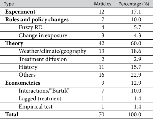
The first category is randomized experiments. These articles employ randomization, designed and conducted by researchers or a third party, and use 2SLS estimation to tackle noncompliance. With random assignment, our confidence in the exogeneity assumption increases because unconfoundedness is guaranteed by design and the direct effect of the instrument on the outcome is easier to rule out than without random assignment. For instance, Alt, Marshall, and Lassen (Reference Alt, Marshall and Lassen2016) use assignment to an information treatment as an instrument for economic beliefs to understand the relationship between economic expectations and vote choice. Compared to IV articles published before 2010, the proportion of articles using experiment-generated IVs has increased significantly (from 2.9% to 17.1%) due to the growing popularity of experiments.
Another category consists of instruments derived from explicit rules on observed covariates, creating quasi-random variations in the treatment. Sovey and Green (Reference Sovey and Green2011) refer to this category as “Natural Experiment.” We avoid this terminology because it is widely misused and limit this category to two circumstances: fuzzy RD designs and variation in exposure to policies due to time of birth or eligibility. For example, Kim (Reference Kim2019) leverages a reform in Sweden that requires municipalities above a population threshold to adopt direct democratic institutions. Dinas (Reference Dinas2014) uses eligibility to vote based on age at the time of an election as an instrument for whether respondents did vote. While rule-based IVs offer a pathway to credible causal inference, recent studies have raised concerns about their implementation, highlighting issues of insufficient power in many RD designs (Stommes, Aronow, and Sävje Reference Stommes, Aronow and Sävje2023).
The next category is “Theory,” where the authors justify unconfoundedness and the exclusion restriction using social science theories or substantive knowledge. Over a decade after Sovey and Green’s (Reference Sovey and Green2011) survey, it remains the most prevalent category among IV studies in political science, at around 60%. We divide theory-based IVs into four subcategories: geography/climate/weather, treatment diffusion, history, and others. First, Many studies in the theory category justify the choices of their instruments based on geography, climate, or weather conditions. For example, Zhu (Reference Zhu2017) uses weighted geographic closeness as an instrument for the activities of multinational corporations; Hager and Hilbig (Reference Hager and Hilbig2019) use mean elevation and distance to rivers to instrument equitable inheritance customs; Henderson and Brooks (Reference Henderson and Brooks2016) use rainfall around Election Day as an instrument for Democratic vote margins. Relatedly, several studies base their choices on regional diffusion of treatment. For example, Dube and Naidu (Reference Dube and Naidu2015) use U.S. military aid to countries outside Latin America as an instrument for U.S. military aid to Colombia. Dorsch and Maarek (Reference Dorsch and Maarek2019) use the regional share of democracies as an instrument for democratization in a country-year panel.Footnote 7 Third, historical instruments derive from past differences between units unrelated to current treatment levels. For example, Vernby (Reference Vernby2013) uses historical immigration levels as an instrument for the current number of noncitizen residents. Finally, several articles rely on a unique instrument based on theories that we could not place in a category. Dower et al. (Reference Dower, Finkel, Gehlbach and Nafziger2018) use religious polarization as an instrument for the frequency of unrest and argue that religious polarization could only impact collective action through its impact on representation in local institutions.
We wish to clarify that our reservations regarding instruments in this category are not primarily about theories themselves. As a design-based approach, the IV strategy requires specific and precise theories about the assignment process of the instruments and the exclusion restriction. We remain skeptical because many “theory”-driven instruments, in our view, do not genuinely uphold these assumptions, often appearing to be developed in an ad hoc or post hoc manner.
The last category of instruments are based on econometric assumptions. This category includes what Sovey and Green (Reference Sovey and Green2011) call “Lags.” These are econometric transformations of variables argued to constitute instruments. For example, Lorentzen, Landry, and Yasuda (Reference Lorentzen, Landry and Yasuda2014) use a measure of the independent variable from eight years earlier to mitigate endogeneity concerns. Another example is shift-share “Bartik” instruments-based. For example, Baccini and Weymouth (Reference Baccini and Weymouth2021) use the interaction between job shares in specific industries and national employment changes to study the effect of manufacturing layoffs on voting. The number of articles relying on econometric techniques, including flawed empirical tests (such as regressing y on d and z and checking if the coefficient of z is significant), has decreased.
4 Replication Procedure and Results
In this section, we describe our replication procedure and report the main findings.
4.1 Procedure
For each paper, we select the main IV specification that plays a central role in supporting a main claim in the paper; it is either referred to as the baseline specification or appears in one of the main tables or figures. Focusing on this specification, our replication procedure involves the following steps. First, we compute the first-stage partial F-statistic based on (1) classic analytic SEs, (2) Huber White heteroskedastic-robust SEs, (3) cluster-robust SEs (if applicable and based on the original specifications), and (4) bootstrapped SEs.Footnote 8
We also calculate $F_{\texttt {Eff}}$
.
$F_{\texttt {Eff}}$
.
We then replicate the original IV result using the 2SLS estimator and apply four different inferential procedures. First, we make inferences based on analytic SEs, including robust SEs or cluster-robust SEs (if applicable). Additionally, we use two nonparametric bootstrap procedures, as described in Section 2, bootstrap-c and bootstrap-t. For specifications with only a single instrument, we also employ the $tF$
procedure proposed by Lee et al. (Reference Lee, McCrary, Moreira and Porter2022), using the 2SLS t-statistic and first-stage F-statistic based on analytic SEs accounting for the originally specified clustering structure. Finally, we conduct an AR procedure and record the p-values and CIs.
$tF$
procedure proposed by Lee et al. (Reference Lee, McCrary, Moreira and Porter2022), using the 2SLS t-statistic and first-stage F-statistic based on analytic SEs accounting for the originally specified clustering structure. Finally, we conduct an AR procedure and record the p-values and CIs.
We record the point estimates, SEs (if applicable), 95% CIs, and p-values for each procedure (the point estimates fully replicate the reported estimates in the original articles and are the same across all procedures). In addition, we estimate a naïve OLS model by regressing the outcome variable on the treatment and covariates, leaving out the instrument. We calculate the ratio between the magnitudes of the 2SLS and OLS estimates, as well as the ratio of their analytic SEs. We also record other useful information, such as the number of observations, the number of clusters, the types of instruments, the methods used to calculate SEs or CIs, and the rationale for each paper’s IV strategy. Our replication yields the following three main findings.
4.2 Finding 1. The First-Stage Partial F-Statistic
Our first finding regards the strengths of the instruments. To our surprise, among the 70 IV designs, 12 (17%) do not report this crucial statistic despite its key role in justifying the validity of an IV design. Among the remaining 58 studies that report F-statistic, 9 (16%) use classic analytic SEs, thus not adjusting for potential heteroskedasticity or clustering structure. In Figure 2, we plot the replicated first-stage partial F-statistic based on the authors’ original model specifications and choices of variance estimators on the x-axis against (a) effective F-statistic or (b) bootstrapped F-statistic on the y-axis, both on a logarithmic scale.Footnote 9
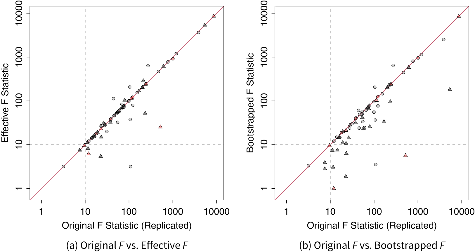
Figure 2 Original versus effective and bootstrapped F. Circles represent applications without a clustering structure and triangles represent applications with a clustering structure. Studies that do not report F-statistic are painted in red. The original F-statistics are obtained from the authors’ original model specifications and choices of variance estimators in the 2SLS regressions. They may differ from those reported in the articles because of misreporting.
In the original studies, the authors used various SE estimators, such as classic SEs, robust SEs, or cluster-robust SEs. As a result, the effective F may be larger or smaller than the original ones. However, a notable feature of Figure 2 is that when a clustering structure exists, the original F-statistic tends to be larger than the effective F or bootstrapped F. When using the effective F as the benchmark, eight studies (11%) have $F_{\texttt {Eff}}<10$
. This number increases to 12 (17%) when the bootstrapped F-statistic is used. The median first-stage
$F_{\texttt {Eff}}<10$
. This number increases to 12 (17%) when the bootstrapped F-statistic is used. The median first-stage $F_{\texttt {Eff}}$
statistic is higher in experimental studies compared to nonexperimental ones (67.7 vs. 53.5). It is well known that failing to cluster the SEs at appropriate levels or using the analytic cluster-robust SE with too few clusters can lead to an overstatement of statistical significance (Cameron, Gelbach, and Miller Reference Cameron, Gelbach and Miller2008). However, this problem has received less attention when evaluating IV strength using the F-statistic.Footnote 10
$F_{\texttt {Eff}}$
statistic is higher in experimental studies compared to nonexperimental ones (67.7 vs. 53.5). It is well known that failing to cluster the SEs at appropriate levels or using the analytic cluster-robust SE with too few clusters can lead to an overstatement of statistical significance (Cameron, Gelbach, and Miller Reference Cameron, Gelbach and Miller2008). However, this problem has received less attention when evaluating IV strength using the F-statistic.Footnote 10
4.3 Finding 2. Inference
Typically, 2SLS estimates have higher uncertainties than OLS estimates. Figure 3 reveals that the 2SLS estimates in the replication sample are in general much less precise than their OLS counterparts, with the median ratio of the analytic SEs equal to 3.8. This ratio decreases as the strength of the instrument, measured by the estimated correlation coefficient between the treatment and predicted treatment $|\hat \rho (d, \hat {d})|$
, increases. This is not surprising because
$|\hat \rho (d, \hat {d})|$
, increases. This is not surprising because $\hat \rho (d, \hat {d})^2 = R_{dz}^2$
, the first-stage partial R-squared. However, one important implication of large differences in SEs is that to achieve comparable levels of statistical significance, 2SLS estimates often need to be at least three times larger than OLS estimates—not to mention that t-testing based on analytical SEs for 2SLS coefficients is often overly optimistic. This difference in precision sets the stage for potential publication bias and p-hacking.
$\hat \rho (d, \hat {d})^2 = R_{dz}^2$
, the first-stage partial R-squared. However, one important implication of large differences in SEs is that to achieve comparable levels of statistical significance, 2SLS estimates often need to be at least three times larger than OLS estimates—not to mention that t-testing based on analytical SEs for 2SLS coefficients is often overly optimistic. This difference in precision sets the stage for potential publication bias and p-hacking.

Figure 3 Comparison of 2SLS and OLS analytic SEs. Subfigure (a) shows the distribution of the ratio between $\hat {SE}(\hat \tau _{2SLS})$
and
$\hat {SE}(\hat \tau _{2SLS})$
and $\hat {SE}(\hat \tau _{OLS})$
, both obtained analytically. Subfigure (b) plots the relationship between the absolute values of
$\hat {SE}(\hat \tau _{OLS})$
, both obtained analytically. Subfigure (b) plots the relationship between the absolute values of $\hat \rho (d, \hat {d})$
, the estimated correlational coefficient between d and
$\hat \rho (d, \hat {d})$
, the estimated correlational coefficient between d and $\hat {d}$
, and the ratio (on a logarithmic scale). In one study, the analytic
$\hat {d}$
, and the ratio (on a logarithmic scale). In one study, the analytic $\hat {SE}(\hat \tau _{2SLS})$
is much smaller than
$\hat {SE}(\hat \tau _{2SLS})$
is much smaller than $\hat {SE}(\hat \tau _{OLS})$
; we suspect that the former severely underestimates the true SE of the 2SLS estimate, likely due to a clustering structure.
$\hat {SE}(\hat \tau _{OLS})$
; we suspect that the former severely underestimates the true SE of the 2SLS estimate, likely due to a clustering structure.
Next, we compare the reported and replicated p-values for the null hypothesis of no effect. For studies that do not report a p-value, we calculate it based on a standard normal distribution using the reported point estimates and SEs. The replicated p-values are based on (1) bootstrap-c, (2) bootstrap-t, and (3) the AR procedure. Since we can exactly replicate the point estimates for the articles in the replication sample, the differences in p-values are the result of the inferential methods used. Figure 4a–c plots reported and replicated p-values, from which we observed two patterns. First, most of the reported p-values are smaller than 0.05 or 0.10, the conventional thresholds for statistical significance. Second, consistent with Young’s (Reference Young2022) finding, our replicated p-values based on the bootstrap methods or AR procedure are usually bigger than the reported p-value (exceptions are mostly caused by rounding errors), which are primarily based on t-statistics calculated using analytic SEs. Using the AR test, we cannot reject the null hypothesis of no effect at the 5% level in 12 studies (17%), compared with 7 (10%) in the original studies. The number increases to 13 (19%) and 19 (27%) when we use p-values from the bootstrap-t and -c methods. Note that very few articles we review utilize inferential procedures specifically designed for weak instruments, such as the AR test (two articles), the conditional likelihood-ratio test (Moreira Reference Moreira2003) (one article), and confident sets (Mikusheva and Poi Reference Mikusheva and Poi2006) (none).
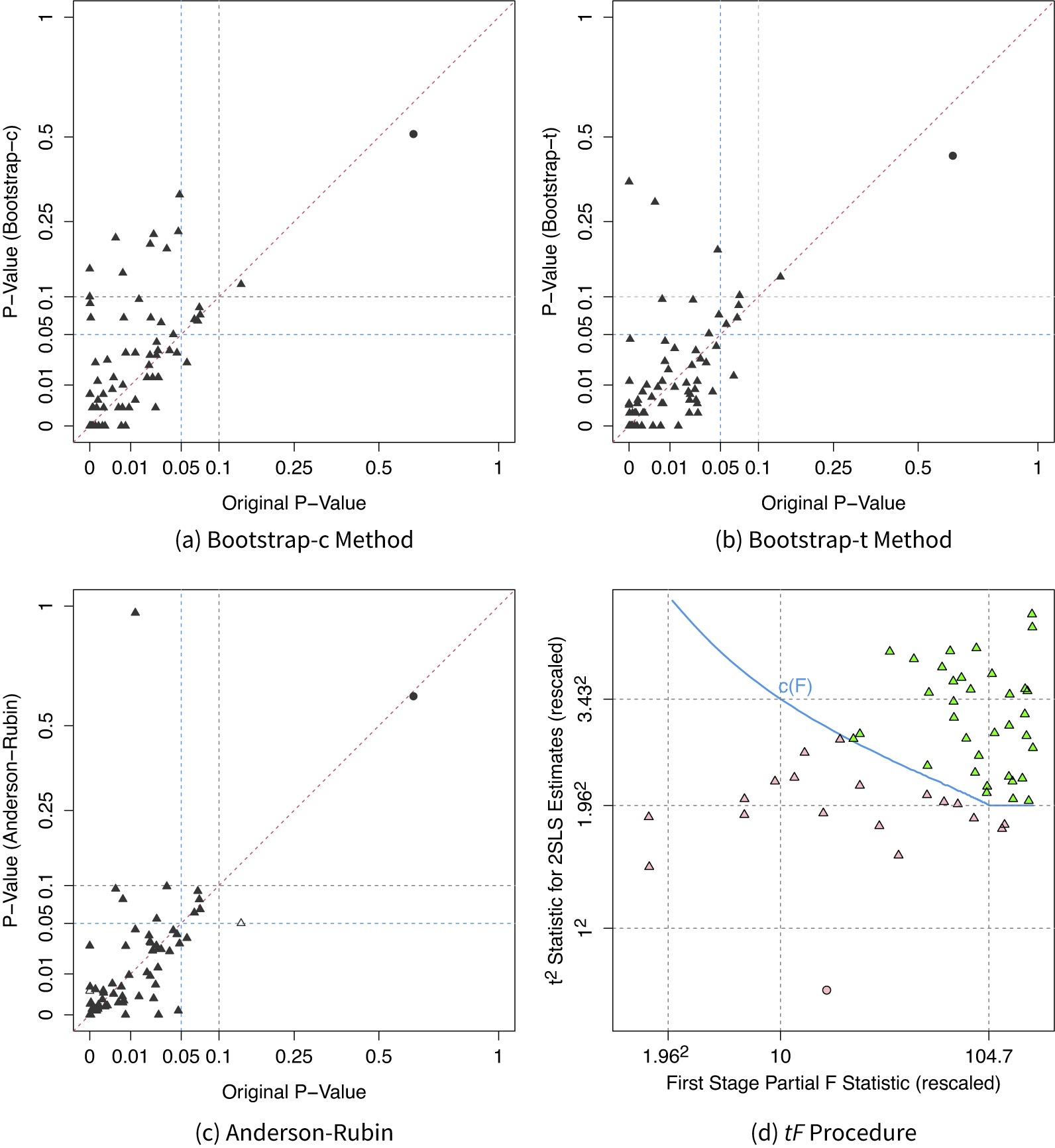
Figure 4 Alternative inferential methods. In subfigures (a)–(c), we compare original p-values to those from alternative inferential methods, testing against the null that $\tau = 0$
. Both axes use a square-root scale. Original p-values are adapted from original articles or calculated using standard-normal approximations of z-scores. Solid circles represent Arias and Stasavage (Reference Arias and Stasavage2019), where the authors argue for a null effect using IV strategy. Bootstrap-c and -t represent percentile methods based on 2SLS estimates and t-statistics, respectively, using original model specifications. Hollow triangles in subfigure (c) indicate unbounded 95% CIs from the AR test using the inversion method. Subfigure (d) presents
$\tau = 0$
. Both axes use a square-root scale. Original p-values are adapted from original articles or calculated using standard-normal approximations of z-scores. Solid circles represent Arias and Stasavage (Reference Arias and Stasavage2019), where the authors argue for a null effect using IV strategy. Bootstrap-c and -t represent percentile methods based on 2SLS estimates and t-statistics, respectively, using original model specifications. Hollow triangles in subfigure (c) indicate unbounded 95% CIs from the AR test using the inversion method. Subfigure (d) presents $tF$
procedure results from 54 single instrument designs. Green and red dots represent studies remaining statistically significant at the 5% level using the
$tF$
procedure results from 54 single instrument designs. Green and red dots represent studies remaining statistically significant at the 5% level using the $tF$
procedure and those that do not, respectively. Subfigures (a)–(c) are inspired by Figure 3 in Young (Reference Young2022), and subfigure (d) by Figure 3 in Lee et al. (Reference Lee, McCrary, Moreira and Porter2022).
$tF$
procedure and those that do not, respectively. Subfigures (a)–(c) are inspired by Figure 3 in Young (Reference Young2022), and subfigure (d) by Figure 3 in Lee et al. (Reference Lee, McCrary, Moreira and Porter2022).
We also apply the $tF$
procedure to 54 studies that use single IVs using
$tF$
procedure to 54 studies that use single IVs using $F_{\texttt {Eff}}$
statistics and t-statistics based on robust or cluster-robust SEs. Figure 4d shows that 19 studies (35%) are not statistically significant at the 5% level, and 7 studies (13%) deemed statistically significant when using the conventional fixed critical values for the t-test become statistically insignificant using the
$F_{\texttt {Eff}}$
statistics and t-statistics based on robust or cluster-robust SEs. Figure 4d shows that 19 studies (35%) are not statistically significant at the 5% level, and 7 studies (13%) deemed statistically significant when using the conventional fixed critical values for the t-test become statistically insignificant using the $tF$
procedure, indicating that overly optimistic critical values due to weak instruments also contribute to overestimation of statistical power, but not as the primary factor. These results suggest that both weak instruments and non-i.i.d. errors have contributed to overstatements of power in IV studies in political science.
$tF$
procedure, indicating that overly optimistic critical values due to weak instruments also contribute to overestimation of statistical power, but not as the primary factor. These results suggest that both weak instruments and non-i.i.d. errors have contributed to overstatements of power in IV studies in political science.
4.4 Finding 3. 2SLS–OLS Discrepancy
Finally, we investigate the relationship between the 2SLS estimates and naïve OLS estimates. In Figure 5a, we plot the 2SLS coefficients against the OLS coefficients, both normalized using reported OLS SEs. The shaded area indicates the range beyond which the OLS estimates are statistically significant at the 5% level. It shows that for most studies in our sample, the 2SLS estimates and OLS estimates share the same direction and that the magnitudes of the former are often much larger than those of the latter. Figure 5b plots the distribution of the ratio between the 2SLS and OLS estimates (in absolute terms). The mean and median of the absolute ratios are 12.4 and 3.4, respectively. In fact, in all but two designs (97%), the 2SLS estimates are bigger than the OLS estimates, consistent with Jiang’s (Reference Jiang2017) finding based on finance research. While it is theoretically possible for most OLS estimates in our sample to be biased toward zero, only 21% of the studies have researchers expressing their belief in downward biases of the OLS estimates. Meanwhile, 40% of the studies consider the OLS results to be their main findings. The fact that researchers use IV designs as robustness checks for OLS estimates due to concerns of upward biases is apparently at odds with the significantly larger magnitudes of the 2SLS estimates.
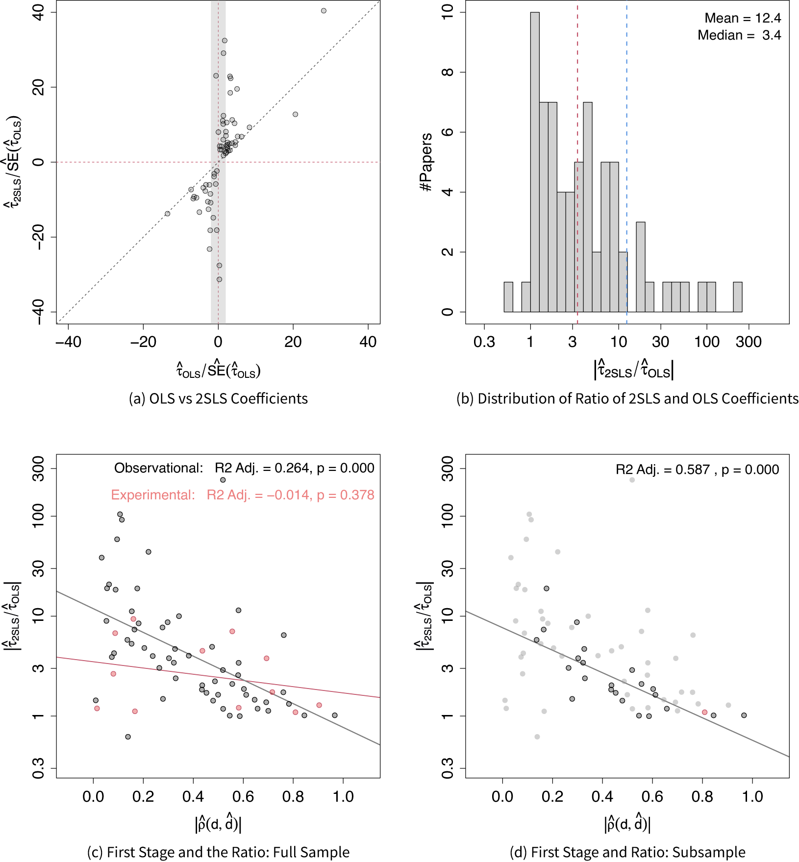
Figure 5 Relationship between OLS and 2SLS estimates. In subfigure (a), both axes are normalized by reported OLS SE estimates with the gray band representing the $[-1.96, 1.96]$
interval. Subfigure (b) displays a histogram of the logarithmic magnitudes of the ratio between reported 2SLS and OLS coefficients. Subfigures (c) and (d) plot the relationship between
$[-1.96, 1.96]$
interval. Subfigure (b) displays a histogram of the logarithmic magnitudes of the ratio between reported 2SLS and OLS coefficients. Subfigures (c) and (d) plot the relationship between $|\hat \rho (d,\hat {d})|$
and the ratio of 2SLS and OLS estimates. Gray and red circles represent observational and experimental studies, respectively. Subfigure (d) highlights studies with statistically significant OLS results at the 5% level, claimed as part of the main findings.
$|\hat \rho (d,\hat {d})|$
and the ratio of 2SLS and OLS estimates. Gray and red circles represent observational and experimental studies, respectively. Subfigure (d) highlights studies with statistically significant OLS results at the 5% level, claimed as part of the main findings.
In Figure 5c, we further explore whether the 2SLS–OLS discrepancy is related to IV strength, measured by $|\hat \rho (d, \hat {d})|$
. We find a strong negative correlation between
$|\hat \rho (d, \hat {d})|$
. We find a strong negative correlation between $|\hat {\tau }_{2SLS} / \hat {\tau }_{OLS}|$
and
$|\hat {\tau }_{2SLS} / \hat {\tau }_{OLS}|$
and $|\hat \rho (d,\hat {d})|$
among studies using nonexperimental instruments (gray dots). The adjusted
$|\hat \rho (d,\hat {d})|$
among studies using nonexperimental instruments (gray dots). The adjusted $R^2$
is
$R^2$
is $0.264$
, with
$0.264$
, with $p = 0.000$
. However, the relationship is much weaker among studies using experiment-generated instruments (red dots). The adjusted
$p = 0.000$
. However, the relationship is much weaker among studies using experiment-generated instruments (red dots). The adjusted $R^2$
is
$R^2$
is $-0.014$
with
$-0.014$
with $p = 0.378$
. At first glance, this result may seem mechanical: as the correlation between d and
$p = 0.378$
. At first glance, this result may seem mechanical: as the correlation between d and $\hat {d}$
increases, the 2SLS estimates naturally converge to the OLS estimates. However, the properties of the 2SLS estimator under the identifying assumptions do not predict the negative relationship (we confirm it in simulations in the SM), and such a relationship is not found in experimental studies. In Figure 5d, we limit our focus to the subsample in which the OLS estimates are statistically significant at the 5% level and researchers accept them as (part of) the main findings, and the strong negative correlation remains.
$\hat {d}$
increases, the 2SLS estimates naturally converge to the OLS estimates. However, the properties of the 2SLS estimator under the identifying assumptions do not predict the negative relationship (we confirm it in simulations in the SM), and such a relationship is not found in experimental studies. In Figure 5d, we limit our focus to the subsample in which the OLS estimates are statistically significant at the 5% level and researchers accept them as (part of) the main findings, and the strong negative correlation remains.
Several factors may be contributing to this observed pattern, including (1) failure of the exogeneity assumption, (2) publication bias, (3) heterogeneous treatment effects, and (4) measurement error in d. As noted earlier, biases originating from endogenous IVs or exclusion restriction failures can be magnified by weak instruments, that is, $\frac {|\text {Bias}_{IV}|}{|\text {Bias}_{OLS}|} = \left |\frac {\text {Cov}(z, \varepsilon )\mathbb {V}\left [d\right ]}{ \text {Cov}(d, \varepsilon )\text {Cov}(z, d)}\right | = \frac {|\rho (z, \varepsilon )|}{|\rho (d, \varepsilon )|\cdot |\rho (d, \hat {d})|} \gg ~1$
. In addressing large IV–OLS estimate ratios, Hahn and Hausman (Reference Hahn and Hausman2005) suggest two explanations: it could stem from a bias in OLS or from a bias in IV due to violations of the exogeneity assumption. Our empirical results, with particularly dubious IV to OLS estimate ratios in nonexperimental studies, seem to align with the latter explanation.
$\frac {|\text {Bias}_{IV}|}{|\text {Bias}_{OLS}|} = \left |\frac {\text {Cov}(z, \varepsilon )\mathbb {V}\left [d\right ]}{ \text {Cov}(d, \varepsilon )\text {Cov}(z, d)}\right | = \frac {|\rho (z, \varepsilon )|}{|\rho (d, \varepsilon )|\cdot |\rho (d, \hat {d})|} \gg ~1$
. In addressing large IV–OLS estimate ratios, Hahn and Hausman (Reference Hahn and Hausman2005) suggest two explanations: it could stem from a bias in OLS or from a bias in IV due to violations of the exogeneity assumption. Our empirical results, with particularly dubious IV to OLS estimate ratios in nonexperimental studies, seem to align with the latter explanation.
Publication bias may have also played a significant role. As shown in Figure 3, the variance of IV estimates increase as $|\hat \rho (d,\skew6\hat{d})|$
diminishes. If researchers selectively report only statistically significant results, or if journals have a tendency to publish such findings, it is not surprising that the discrepancies between IV and OLS estimates widen as the strength of the first stage declines, as shown in Figure 5c,d. This is because 2SLS estimates often need to be substantially larger than OLS estimates to achieve statistical significance. This phenomenon is known as Type-M bias and has been discussed in psychology and sociology literature (Felton and Stewart Reference Felton and Stewart2022; Gelman and Carlin Reference Gelman and Carlin2014). Invalid instruments exacerbate this issue by providing ample opportunities for generating such large estimates.
$|\hat \rho (d,\skew6\hat{d})|$
diminishes. If researchers selectively report only statistically significant results, or if journals have a tendency to publish such findings, it is not surprising that the discrepancies between IV and OLS estimates widen as the strength of the first stage declines, as shown in Figure 5c,d. This is because 2SLS estimates often need to be substantially larger than OLS estimates to achieve statistical significance. This phenomenon is known as Type-M bias and has been discussed in psychology and sociology literature (Felton and Stewart Reference Felton and Stewart2022; Gelman and Carlin Reference Gelman and Carlin2014). Invalid instruments exacerbate this issue by providing ample opportunities for generating such large estimates.
Moreover, 30% of the replicated studies in our sample mention heterogeneous treatment effects as a possible explanation for this discrepancy. OLS and 2SLS place different weights on covariate strata in the sample, and therefore if compliers, those whose treatment status is affected by the instrument, are more responsive to the treatment than the rest of the units in the sample, we might see diverging OLS and 2SLS estimates. Under the assumption that the exclusion restriction holds, this gap can be decomposed into covariate weight difference, treatment-level weight difference, and endogeneity bias components using the procedure developed in Ishimaru (Reference Ishimaru2021). In the SM, we investigate this possibility and find that it is highly unlikely that heterogeneous treatment effects alone can explain the difference in magnitudes between 2SLS and OLS estimates we observe in the replication data, that is, the variance in treatment effects needed for this gap is implausibly large.
Finally, IV designs can correct for downward biases due to measurement errors in d, resulting in $|\hat {\tau }_{2SLS} / \hat {\tau }_{OLS}|> 1$
. If the measurement error is large, this can weaken the relationship between d and
$|\hat {\tau }_{2SLS} / \hat {\tau }_{OLS}|> 1$
. If the measurement error is large, this can weaken the relationship between d and $\skew6\hat{d}$
, producing a negative correlation. We find it an unlikely explanation because only four articles (6%) attribute their use of IV to measurement errors, and the negative correlation is even stronger when we focus solely on studies where OLS estimates are statistically significant and regarded as the main findings.
$\skew6\hat{d}$
, producing a negative correlation. We find it an unlikely explanation because only four articles (6%) attribute their use of IV to measurement errors, and the negative correlation is even stronger when we focus solely on studies where OLS estimates are statistically significant and regarded as the main findings.
In Table 3, we present a summary of the main findings from our replication exercise. Observational studies, compared to experimental counterparts, generally have weaker first stages, often display larger increases in p-values when more robust inferential methods are used, and demonstrate bigger discrepancies between the 2SLS and OLS estimates. Based on these findings, we contend that a significant proportion of IV results based on observational data in political science either lack credibility or yield estimates that are too imprecise to offer insights beyond those provided by OLS regressions.
Table 3 Summary of replication results

5 Recommendations
IV designs in experimental and observational studies differ fundamentally. In randomized experiments, the instruments’ unconfoundedness is ensured by design, and researchers can address possible exclusion restriction violations at the design stage, for example, by testing potential design effects through randomization (Gerber and Green Reference Gerber and Green2012, 140–141). Practices like power analysis, placebo tests, and preregistration also help reduce the improper use of IVs. In contrast, observational IV designs based on “natural experiments” require detailed knowledge of the assignment mechanism, making them more complex and prone to issues (Sekhon and Titiunik Reference Sekhon and Titiunik2012).
Our findings suggest that using an IV strategy in observational settings is extremely challenging due to several reasons. First, truly random and strong instruments are rare and difficult to find. This is mainly because neither unconfoundedness nor the exclusion restriction is guaranteed by design, placing a greater burden of proof on researchers for the exogeneity assumption. Moreover, conducting placebo tests like the ZFS test for the exclusion restriction after data collection is not always feasible. Finally, increasing the sample size to achieve sufficient statistical power is often impractical. To prevent misuse of IVs in observational studies, we provide a checklist for researchers to consider when applying or contemplating an IV strategy with one endogenous treatment variable:
-
Design
-
• Prior to using an IV strategy, consider how selection bias may affect treatment effect estimates obtained through OLS. If the main concern is underestimating an already statistically significant treatment effect, an IV strategy may be unnecessary.
-
• During the research design phase, consider whether the chosen instrument can realistically create random or quasi-random variations in treatment assignment while remaining excluded from the outcome equation.
-
Characterizing the first stage
-
• Calculate and report $F_{\texttt {Eff}}$
for the first stage, taking into account heteroscedasticity and clustering structure as needed. However, do not discard a design simply because
$F_{\texttt {Eff}}< 10$
.
$F_{\texttt {Eff}}$
for the first stage, taking into account heteroscedasticity and clustering structure as needed. However, do not discard a design simply because
$F_{\texttt {Eff}}< 10$
. -
• If both d and z are continuous, we recommend plotting d against its predicted values,
$\hat {d}$
, after accounting for covariates. Alternatively, plot both d and
$\hat {d}$
against specific covariates that serve as the foundation for the rules used to derive the instruments. These visualizations are useful for detecting outliers and gaining insights into the sources of exogenous variation. -
Hypothesis testing and inference
-
• Option 1. t-test with
$F_{\texttt {Eff}}$
pretesting. If
$F_{\texttt {Eff}} < 10$
, choose Option 2 or 3. Utilize conservative methods like bootstrap-t and bootstrap-c if outliers or group structures are present. -
• Option 2.
$tF$
procedure. For single treatment and instrument cases, adjust t-test critical values based on
$F_{\texttt {Eff}}$
. -
• Option 3. Direct testing. Apply weak-instrument-robust procedures, such as the AR test.
-
Communicating your findings
-
• Present OLS and IV estimates alongside CIs from various inferential methods in a graphical format, like in Figure 6. These CIs may not concur on statistical significance, but they collectively convey the findings’ robustness to different inferential approaches. In addition, they present the degree of uncertainty in both OLS and IV estimates in an intuitive manner.
Figure 6 Replicated OLS and 2SLS estimates with 95% CIs (Rueda Reference Rueda2017, Table 5 column 1). The outcome is citizens’ reports of voting buying. The treatment is the actual polling place size. The instrument is the size of the polling station predicted by the rules limiting the voters per polling station. The magnitude of the 2SLS estimate is slightly larger than that of the OLS estimate. Similar figures for each of the 70 IV designs are shown in the SM. This plot is made by ivDiag, an open-source package in R (Note to editor, please remove the Github link; please format the font of “R” properly).
-
• Remember to report first-stage and reduced-form estimation results, including 95% CIs for coefficients, as they offer insight into both instrument strength and statistical power.
-
Additional diagnostics
-
• If you expect the OLS results to be upward biased, be concerned if the 2SLS estimator yields much larger estimates than OLS.
-
• If there is good reason to believe that treatment effects on compliers are significantly larger in magnitude than those on noncompliers, explain this through profiling of these principal strata (Abadie Reference Abadie2003; Marbach and Hangartner Reference Marbach and Hangartner2020).
-
• If it is possible to identify “never takers” or a subset of them, conduct a placebo test by estimating the effect of the instruments on the outcome in this ZFS sample. Using results from the ZFS test, obtain local-to-zero IV estimates and CIs and compare them to the original estimates. Section A3 of the SM provides detailed explanations and an empirical example.
-
• Conduct a sensitivity analysis as proposed by Cinelli and Hazlett (Reference Cinelli and Hazlett2022).


We provide an R package, ivDiag, to implement our recommended procedures. Stata tutorials for carrying out these procedures are also available on the corresponding author’s website. Our aim is to address concerns regarding IVs in social science research and improve the quality of estimation and inference, especially for nonexperimental IV designs.
Acknowledgements
We thank Te Bao, Thomas Cao, Albert Chiu, Daniel Chen, Gary Cox, Charles Crabtree, Ted Enamorado, Hanming Fang, Avi Feller, Don Green, Justin Grimmer, Anna Grzymala-Busse, Jens Hainmueller, Guido Imbens, David Laitin, Adeline Lo, Justin McCrary, Jacob Montgomery, Doug Rivers, Henrik Sigstad, Brandon Stewart, Arthur Yu, and Xiang Zhou, as well as seminar participants at Stanford University, Washington University in St. Louis, APSA 2021, and Polmeth 2021, for their extremely helpful comments. We are also deeply grateful to four anonymous reviewers for PA and Editor Jeff Gill, as well as two anonymous reviewers for APSR—their invaluable suggestions have improved this paper significantly.
Data Availability Agreement
Replication data and code for this article have been published at Harvard Dataverse at https://doi.org/10.7910/DVN/MM5THZ.
Supplementary Material
For supplementary material accompanying this paper, please visit https://doi.org/10.1017/pan.2024.2.


 Open access