


1. Introduction
The jets launched from a radio-loud active galactic nucleus (AGN) arise from the accretion onto a supermassive black hole and form synchrotron-emitting radio lobes in the intergalactic environments of their host galaxies (Scheuer Reference Scheuer1974). While the jets are active, a radio galaxy will often display compact features such as an unresolved radio core coincident with its host galaxy, bipolar jets, and hotspots in the lobes of Fanarof–Riley type II (FR-II; Fanaroff & Riley Reference Fanaroff and Riley1974) radio galaxies. The radio continuum spectrum arising from the lobes is usually well approximated by a broken power law for radio frequencies between 100 MHz and 10 GHz; the observed spectral index,  $\alpha$Footnote a, typically ranges within $-1.0<\alpha<-0.5$. Steepening in the radio lobe spectrum is allowed by $\Delta \alpha\leq0.5$ (e.g. the CI model; Kardashev Reference Kardashev1962; Pacholczyk Reference Pacholczyk1970; Jaffe & Perola Reference Jaffe and Perola1973) and is attributed to ageing of the lobe plasma.
Such active radio galaxies do not offer a complete picture to the life cycle of radio galaxies due to a seemingly intermittent behaviour of the AGN jet activity. The remnant phase of a radio galaxy begins once the jets switch off. During this phase, the lobes will fade as they undergo a rapid spectral evolution, for example, as shown observationally by Murgia et al. (Reference Murgia2011), Shulevski et al. (Reference Shulevski, Morganti, Oosterloo and Struve2012), Godfrey, Morganti, & Brienza (Reference Godfrey, Morganti and Brienza2017), Brienza et al. (Reference Brienza2017), Mahatma et al. (Reference Mahatma2018), Jurlin et al. (Reference Jurlin2020) and shown with modelling conducted by Turner (Reference Turner2018), Hardcastle (Reference Hardcastle2018) and Shabala et al. (Reference Shabala2020). Remnant radio galaxies, remnants herein, will remain observable for many tens of Myr at low ( $\sim150$ MHz) frequencies, which is comparable but shorter than the duration of their previous active phase (Shulevski et al. Reference Shulevski2017; Turner Reference Turner2018; Brienza et al. Reference Brienza2020). Jets are also known to restart after a period of inactivity (e.g. Roettiger et al. Reference Roettiger, Burns, Clarke and Christiansen1994), giving rise to a restarted radio galaxy. Several observational classes exist to describe such sources; double–double radio galaxies (Schoenmakers et al. Reference Schoenmakers, de Bruyn, Röttgering, van der Laan and Kaiser2000) describe sources in which two distinct pairs of lobes can be observed; however, restarting jets can also appear as compact steep-spectrum sources embedded within larger-scale remnant lobes (e.g. Brienza et al. Reference Brienza2018).
Compiling samples of remnant (Saripalli et al. Reference Saripalli, Subrahmanyan, Thorat, Ekers, Hunstead, Johnston and Sadler2012; Godfrey et al. Reference Godfrey, Morganti and Brienza2017; Brienza et al. Reference Brienza2017; Mahatma et al. Reference Mahatma2018) and restarted (Saripalli et al. Reference Saripalli, Subrahmanyan, Thorat, Ekers, Hunstead, Johnston and Sadler2012; Mahatma et al. Reference Mahatma2019) radio galaxies sheds new light on their dynamics and evolution, and by extension, the AGN jet duty cycle. Jurlin et al. (Reference Jurlin2020) present a direct analysis of the radio galaxy life cycle, in which their sample is decomposed into active, remnant, and restarted radio galaxies. To complement these observational works, Shabala et al. (Reference Shabala2020) present a new methodology in which uniformly selected samples of active, remnant, and restarted radio galaxies are used to constrain evolutionary models describing the AGN jet duty cycle.
However, using radio observations to confidently identify radio sources in these phases is a challenging task, even in the modern era of radio instruments. Remnant radio galaxies, which are the focus of this work, display various observational properties that correlate with age, presenting a challenge for identifying complete samples of such sources. Various selection techniques exist amongst the literature, each with their selection biases. Due to the preferential cooling of higher-energy synchrotron-radiating electrons (Jaffe & Perola Reference Jaffe and Perola1973; Komissarov & Gubanov Reference Komissarov and Gubanov1994), many authors have identified remnants by their ultra-steep radio spectrum ( $\alpha<-1.2$), reflecting the absence of a source of energy injection, e.g. Cordey (Reference Cordey1987), Parma et al. (Reference Parma, Murgia, de Ruiter, Fanti, Mack and Govoni2007), and Hurley-Walker et al. (Reference Hurley-Walker2015). However, Brienza et al. (Reference Brienza2016) demonstrate that this technique preferentially selects aged remnants and will miss those in which the lobes have not had time to steepen over the observed frequency range. Murgia et al. (Reference Murgia2011) propose a spectral curvature (SPC) criterion, which evaluates the difference in spectral index over two frequency ranges, for example, SPC = $\alpha_{\mathrm{high}}$ - $\alpha_{\mathrm{low}}$ such that SPC $>$0 for a convex spectrum. Sources with SPC $>0.5$ demonstrate highly curved spectra and are likely attributed to remnant lobes. However, modelling conducted by Godfrey et al. (Reference Godfrey, Morganti and Brienza2017) shows that not all remnants will be selected this way, even at high ( $\sim$10 GHz) frequencies.
Morphological selection offers a complementary way to identify remnants, independent of spectral ageing of the lobes. This technique often involves searching for low surface brightness (SB) profiles (SB  $<50$ mJy arcmin–2), amorphous radio morphologies, and an absence of hotspots (e.g. Saripalli et al. Reference Saripalli, Subrahmanyan, Thorat, Ekers, Hunstead, Johnston and Sadler2012; Brienza et al. Reference Brienza2017). However, young remnants in which the hotspots have not yet disappeared due to a recent switch off of the jets (e.g. 3C 028; Feretti et al. Reference Feretti, Gioia, Giovannini, Gregorini and Padrielli1984; Harwood et al. Reference Harwood, Hardcastle and Croston2015) will be missed with these techniques.
An alternative approach is to identify remnants based on an absent radio core; a radio core should be absent if the AGN is currently inactive (Giovannini et al. Reference Giovannini, Feretti, Gregorini and Parma1988). This property is often invoked to confirm the status of a remnant radio galaxy, for example, see Cordey (Reference Cordey1987), and is recently employed by Mahatma et al. (Reference Mahatma2018) as a criterion to search for remnant candidates in a LOw Frequency ARray (LOFAR)-selected sample. The caveat here is the plausibility for a faint radio core to exist below the sensitivity of the observations, meaning this method selects only for remnant candidates. This method will also miss remnant lobes from a previous epoch of activity in restarted radio galaxies. A likely example of such a source is MWA Interestingly Deep Astrophysical Survey (MIDAS) J230304–323228, discussed in Section 3. These sources are beyond the scope of this work; however, they are a promising avenue for future work.
A common aspect of almost all previously mentioned observational studies of remnant radio galaxies is their selection at low frequencies (typically around 150 MHz). The preferential radiating of high-energy electrons means that the observable lifetime of remnant lobes increases at a lower observing frequency. Incorporating a low-frequency selection thus plays an important role in improving the completeness of remnant radio galaxy samples; quite often the oldest remnant lobes are detectable only at such low frequencies.
In this work, we take advantage of a broad range of radio surveys targeting the Galaxy And Mass Assembly (GAMA; Driver et al. Reference Driver2011) 23 field to identify and study new remnant radio galaxies candidates in which the central AGN is currently inactive. We use new low-frequency observations provided by the Murchison Widefield Array (MWA; Tingay et al. Reference Tingay2013) and the Australian Square Kilometre Array Pathfinder (ASKAP; Johnston et al. Reference Johnston2007; McConnell et al. Reference McConnell2016) to compile a sample of radio galaxies and use high-frequency (5.5 GHz) observations provided by the Australia Telescope Compact Array (ATCA) to identify remnant candidates by the ‘absent radio core’ criterion. In Section 2, we present the multi-wavelength data used for this work. In Section 3, we discuss the compilation of our radio galaxy sample, the classification of remnant candidates, and the matching of host galaxies. In Section 4, we discuss each of the selected remnant candidates. In Section 5, we discuss the observed radio properties of the sample and emphasise the caveats of various remnant selection methods. We also discuss the rest-frame properties of the sample, present the fraction of remnants constrained by our observations, and examine a particularly interesting remnant with detailed modelling. Finally, our results are concluded in Section 6.
We assume a flat  $\Lambda$CDM cosmology with $H_0=67.7 $ kms–1 Mpc–1, $\Omega_{\rm M}$=0.307, and $\Omega_\Lambda$=1- $\Omega_{\rm M}$ (Planck Collaboration et al. 2014). All coordinates are reported in the J2000 equinox.
2. Data
Our sample is focused on a 8.31 deg $^2$ subregion of the GAMA 23 field (
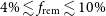
 $\mathrm{RA}=345^\circ,\mathrm{Dec}=-32.5^\circ$), for example, see Figure 1. The rich multi-wavelength coverage makes the absent radio-core criterion a viable method to search for remnant radio galaxies and allows us to match the radio sample with their host galaxies.
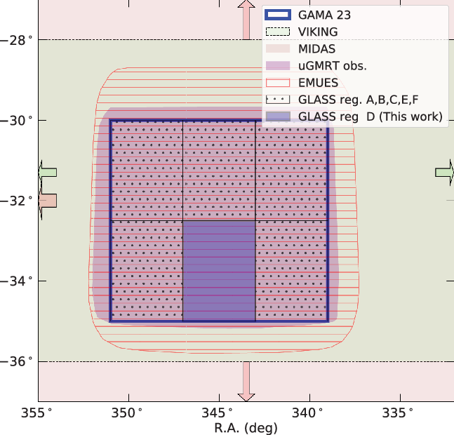
Figure 1. Sky coverage of radio surveys dedicated to observing GAMA 23, described in Section 2.1. Near-infrared VIKING observations (Section 2.2.1) are also displayed. Thick-red and thin-green arrows indicate the directions in which MIDAS ES and VIKING extend beyond the represented footprint.
Table 1. Summarised properties of the radio surveys spanning the GAMA 23 field. Each column, in ascending order, details the telescope used to conduct the observations, the name of the radio survey, the dates observations that were conducted, the central frequency of the observing band, the bandwidth available in each band, the average noise properties within region D, and the shape of the restoring beam.
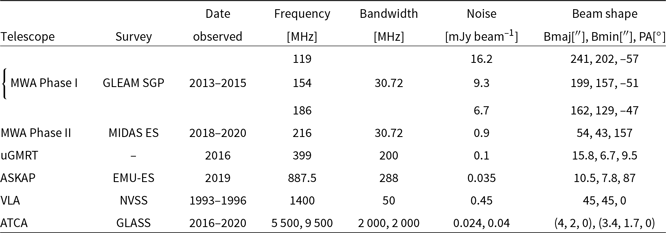
Table 2. Details of the additional ATCA data collected here under project code C3335, PI: B. Quici. Each column, in ascending order, details the configuration used to conduct observations, the date observations were conducted, the central frequency of the receiver band, the bandwidth available within each band, the approximate time spent per source in each configuration, the secondary calibrator observed, the average noise per pointing, and the shape of the restoring beam. Note, primary calibrator PKS B1934-638 was observed for all observations.

2.1. Radio data
Below, we describe the radio observations used throughout this work and they are summarised in Tables 1 and 2.
2.1.1. GLEAM SGP (119, 154, 185 MHz)
From 2013 to 2015, the MWA observed  $\sim$30 000 deg $^2$ of the sky south of Dec $= 30^\circ$. The GaLactic and Extra-galactic All-sky MWA (GLEAM; Wayth et al. Reference Wayth2015) survey adopted a drift scan observing method using the MWA Phase I configuration and a maximum baseline of $\sim$3 km. Observations exclusive to 2013–2014 (year 1) were used to generate the public extra-galactic GLEAM first release (Hurley-Walker et al. Reference Hurley-Walker2017)Footnote b. GLEAM spans a 72–231 MHz frequency range, divided evenly into 30.72-MHz widebands centred at $\nu_c=$ {88, 119, 154, 185, 216} MHz. Observations conducted during 2014–2015 (year 2) covered the same sky area as GLEAM, but with a factor of 2 increase in the observing time due to offset ( $\pm$1 h in median RA) scans. Within a footprint of: 310 $^\circ \leq$ RA $\leq 76^\circ$, –48 $^\circ \leq$ Dec $\leq -2^\circ$ ( $\sim5\,100$ deg $^2$ sky coverage), Franzen et al. (in prep) independently reprocessed the overlapping observations from both years to produce the GLEAM South Galactic Pole (SGP) survey, achieving a factor $\sim3$ increase in integration time over GLEAM. Due to calibration errors associated with Fornax A and Pictor A entering the primary beam sidelobes, the lowest wideband centred at 88 MHz was discarded at imaging. Despite its declination dependence, the GLEAM SGP root-mean-square (RMS) remains effectively constant within the footprint of our (8.31 deg $^2$) study. The point spread function (PSF) varies slightly across the survey; at 216 MHz, the PSF size within GAMA 23 is approximately 150 arcsec $\times$ 119 arcsec, and an RMS of $\sigma \sim 4\pm0.5$ mJy beam-1 is achieved. This is consistent with a factor $ 2$ increase in sensitivity over GLEAM. We use an internal GLEAM SGP component catalogue, developed by the method used for GLEAM. Franzen et al. (in prep) quote an 8% absolute uncertainty in the GLEAM SGP flux density scale, consistent with the value reported for GLEAM by Hurley-Walker et al. (Reference Hurley-Walker2017).
2.1.2. MIDAS ES (216 MHz)
In 2018, the MWA was reconfigured into an extended baseline configuration (MWA Phase II; Wayth et al. Reference Wayth2018). The MWA Phase II provides a maximum baseline of 5.3 km which, at 216 MHz, improves the angular resolution to 54 arcsec  $\times$ 43. This drives down the classical and sidelobe confusion limits, allowing for deeper imaging to be made with an RMS of $\sigma\ll 1\,$mJy beam–1. MWA Phase II science is presented in Beardsley et al. (Reference Beardsley2020). The MWA Interestingly Deep Astrophysical Survey (MIDAS, Seymour et al. in prep) will provide deep observations of six extra-galactic survey fields, including GAMA 23, in the MWA Phase II configuration. Here, we use an early science (MIDAS ES herein) image of the highest frequency band centered at 216 MHz. Data reduction followed the method outlined by Franzen et al. (in prep) where each snapshot was calibrated using a model derived from GLEAM. Imaging was performed using the WSClean imaging software (Offringa et al. Reference Offringa2014) using a robustness of 0 (Briggs Reference Briggs1995). Altogether, 54 2-min snapshot images, each achieving an average RMS of $\sim 8\,$mJy beam–1 without self-calibration, were mosaiced to produce a deep image. Stacking of individual snapshots reproduced the expected $\sqrt{t}$ increase in sensitivity, where t is the total integration time, and implied the classical and sidelobe confusion limits were not reached. After a round of self-calibration, the final deep image, at zenith, achieved an RMS of $\sim$0.9 mJy beam–1 with a $\lesssim1$ arcmin restoring beam. Radio sources were catalogued using the Background And Noise Estimation tool bane, to measure the direction-dependent noise across the image, and aegean to perform source finding and characterisation (Hancock et al. Reference Hancock, Murphy, Gaensler, Hopkins and Curran2012; Hancock, Trott, & Hurley-Walker Reference Hancock, Trott and Hurley-Walker2018)Footnote c. Using the GLEAM catalogue, sources above 10 $\sigma$ in MIDAS ES and GLEAM were used to correct the MIDAS ES flux scale. For 887 such sources in GAMA 23, correction factors were derived based on the integrated flux density ratio between MIDAS ES and GLEAM. The correction factors followed a Gaussian distribution and indicated an agreement with GLEAM within 5%. Given the 8% uncertainty in the GLEAM flux density scale (Section 2.1.1), we prescribe an 8% uncertainty in the MIDAS ES flux density scale.
2.1.3. EMU early science (887 MHz)
In 2019, the ASKAP delivered the first observations conducted with the full 36-antenna array configuration. The design of ASKAP opens up a unique parameter space for studying the extra-galactic radio source population. With a maximum baseline of 6 km, ASKAP produces images with  $\sim 10$ arcsec resolution at 887 MHz. The shortest baseline is 22 m, recovering maximum angular scales of $\sim0.8^\circ$. As part of the Evolutionary Map of the Universe (EMU; Norris Reference Norris2011) Early Science, the GAMA 23 field was observed at 887 MHz and made publicly available on the CSIRO ASKAP Science Data Archive (CASDAFootnote d). Details of the reduction are briefly summarised here. These data have been reduced by the ASKAP collaboration using the ASKAPsoftFootnote e data reduction pipeline (Whiting et al. in prep) on the Galaxy supercomputer hosted by the Pawsey Supercomputing Centre. PKS B1934-638 was used to perform bandpass and flux calibration for each of the unique 36 beams. Bandpass solutions were applied to the target fields. The final images are restored with a 10.55 arcsec $\times$ 7.82 arcsec (BPA = 86.8 $^\circ$) elliptical beam and achieves an RMS of $\sigma \approx 34-45 \upmu$Jy beam–1. Henceforth, we refer to these observations as EMU-ES.
2.1.4. NVSS (1.4 GHz)
We use observations conducted by the National Radio Astronomy Observatory (NRAO) using the Very Large Array (VLA; Thompson et al. Reference Thompson, Clark, Wade and Napier1980) to sample an intermediate frequency range. The NRAO VLA Sky Survey (NVSS; Condon et al. Reference Condon, Cotton, Greisen, Yin, Perley, Taylor and Broderick1998)Footnote f surveys the entire sky down to Dec $=-40^\circ$ at 1400 MHz. Observations for NVSS were collected predominately in the D configuration; however, the DnC configuration was used for Southern declinations. Final image products were restored using a circular synthesised beam of 45 arcsec $\times45$ arcsec. At 1400 MHz, NVSS achieves an RMS of $\sigma=0.45\,$mJy beam–1.
2.1.5. GLASS (5.5 & 9.5 GHz)
The GAMA Legacy ATCA Sky Survey (GLASS; Huynh et al. in prep) offers simultaneous, high-frequency (5.5, 9.5 GHz) observations of GAMA 23 observed by the ATCA. Observations for GLASS were conducted over seven semesters between 2016 and 2020 (PI: M. Huynh, project code: C3132). Data at each frequency were acquired with a 2-GHz bandwidth, made possible by the Compact Array Broadband Backend (Wilson et al. Reference Wilson2011), with the correlator set to a 1-MHz spectral resolution. Observations for GLASS were conducted in two separate ATCA array configurations, the 6A and 1.5C configurations, contributing 69% and 31% towards the total awarded time, respectively. The shortest interferometer spacing is 77 m in the 1.5C configuration, providing a largest recoverable angular scale of 146 arcsec at 5.5 GHz. As part of the observing strategy, GLASS was divided into six 8.31 deg $^2$ regions (regions A–F), for which region D (RA = 345 $^\circ$, Dec = –33.75 $^\circ$) was observed, reduced, and imaged first. For this reason, this paper focuses only on region D.
Processing and data reduction were conducted using the Multichannel Image Reconstruction, Image Analysis and Display (MIRIAD) software package (Sault, Teuben, & Wright Reference Sault, Teuben, Wright, Shaw, Payne and Hayes1995), similar to the method outlined by Huynh et al. (Reference Huynh, Bell, Hopkins, Norris and Seymour2015; Reference Huynh, Seymour, Norris and Galvin2020). The 1435 region D pointings are restored with the Gaussian fit of the dirty beam and convolved to a common beam of 4 arcsec  $\times$ 2 arcsec (BPA = $0^\circ$) at 5.5 GHz and achieves an RMS of $\sim 24\,\upmu$Jy beam–1. A similar process at 9.5 GHz results in a 3.4 arcsec $\times$ 1.7 arcsec (BPA = $0^\circ$) synthesised beam and achieves an RMS of $\sim 40\,\upmu$Jy beam–1. Although the same theoretical sensitivity is expected at 5.5 and 9.5 GHz, the sparse overlap in adjacent pointings, larger phase calibration errors, and increased radio frequency interference (RFI) all result in a drop in sensitivity. Henceforth, we refer to GLASS observations conducted at 5.5 and 9.5 GHz as GLASS 5.5 and GLASS 9.5, respectively.
2.1.6. uGMRT legacy observations (399 MHz)
As part of the GLASS legacy survey (Section 2.1.5), the upgraded Giant Meterwave Telescope (uGMRT) has observed GAMA 23 in band-3 (250–500 MHz) centred at 399 MHz. The project  $32\_060$ (PI: Ishwara Chandra) was awarded 33 h to cover 50 contiguous pointings spanning a 50 square-degree region. Observations were conducted in a semi-snapshot mode, with $\approx 30$ min per pointing distributed through three 10-min scans. In band-3, the wideband correlator collects a bandwidth of 200 MHz divided into 4 000 fine channels. Data reduction was conducted using a Common Astronomical Software Application (CASA; McMullin et al. Reference McMullin, Waters, Schiebel, Young, Golap, Shaw, Hill and Bell2007) pipelinFootnote g. Data reduction followed the standard data reduction practices such as data flagging, bandpass and gain calibration, application of solutions to target scans, imaging and self-calibration (see Ishwara-Chandra et al. Reference Ishwara-Chandra, Taylor, Green, Stil, Vaccari and Ocran2020 for details). The image is restored by a 15.8 arcsec $\times$ 6.71 arcsec (BPA= 9.5 $^\circ$) beam and achieves the best RMS of $\sim$100 $\upmu$ Jy beam–1. Note that several bright sources throughout the field adversely impact the data reduction, resulting in large spatial variations in the RMS.
2.1.7. Low-resolution ATCA observations (2.1, 5.5 & 9 GHz)
Due to their power law spectral energy distributions, the integrated luminosities of radio galaxy lobes decrease with increasing frequency (Section 1). Given that remnants can display ultra-steep radio spectra, this presents a sensitivity challenge associated with their detection. For a survey such as GLASS which has high  $\theta\sim5$ arcsec resolution (Section 2.1.5), resolution bias further exacerbates this problem: diffuse low SB regions escape detection with greater ease, resulting in an under-estimation of the integrated flux density. To combat the resolution bias suffered by GLASS, we carried out low-resolution observations with ATCA.
The project C3335 (PI: B. Quici) was awarded 14 h to conduct low-resolution observations of each remnant identified for this work, at 2.1, 5.5, and 9 GHz. Observations at 2.1 GHz (LS band) were conducted in the H168 configuration; observations at 5.5 and 9 GHz (CX band) were conducted in the H75 configuration. The minimum and maximum baselines achieved within each configuration are 61 and 192 m for H168 and 31 and 89 m for H75, respectively (excluding baselines formed with antenna CA06). Bandpass, gain, and flux calibration was performed using PKS B1934-638. Due to the small angular separation between each target, the secondary calibrator was held constant for each target. At 2.1 GHz, PKS B2259-375 was used for phase calibration. At 5.5 and 9 GHz, phase calibration was performed with PKS B2254-367. To maximise uv coverage, each target was observed on a rotating block of length  $\sim$30 min, with approximatelyFootnote h 2 min allocated per target per block. Secondary calibrators were observed twice per block to ensure stable phase solutions.
Data reduction was performed using the CASA software packageFootnote i and followed the standard data reduction practices. As part of preliminary flagging, the data are ‘clipped’, ‘shadowed’, and ‘quacked’ using the flagdata task, in order to flag for zero values, shadowed antennas, and the first 5 s of the scans, respectively. Forty edge channels of the original 2049 are also flagged due to bandpass roll-off (Wilson et al. Reference Wilson2011). Again using the flagdata task, the uncalibrated data are then automatically flagged for RFI using mode=‘tfcrop’, which calculates flags based on a time and frequency window. The data are manually inspected in an amplitude versus channel space to ensure RFI is adequately flagged. Observations conducted in the LS band and CX band were split into four and eight subbands, respectively. Calibration was performed per subband per pointing. To perform calibration, the complex gains and bandpass are solved for first using the primary calibrator. Complex gains and leakages were solved for next using the secondary calibrator. After applying a flux-scale correction based on PKS B1934-638, the calibration solutions were copied individually to each target scan. A secondary round of automatic RFI flagging is performed with flagdata where mode=‘rflag’, which is used for calibrated data. The primary and secondary calibrator, as well as each target scan, are flagged in this way. In total, approximately  $\approx52\%$ and $\approx 15\%$ of the available bandwidth were flagged due to RFI present in the LS and CX bands, respectively. Within the hybrid configurations, the first five antennas, CA01–CA05, provide the dense packing of short (10–100 m) spacings. Antenna CA06 is fixed and provides much larger spacings of $\sim$4500 m. Given that this results in a large gap in the uv coverage, all baselines formed with antenna CA06 are excluded to achieve a well-behaved point spread function. The average noise properties and restoring beams at 2.1, 5.5, and 9 GHz are, respectively, $\sigma \sim0.7$ mJy beam–1 and $\theta=104\, {\rm arcsec} \times127\, {\rm arcsec}$, $\sigma \sim0.22$ mJy beam–1 and $88\,{\rm arcsec}\times110\,{\rm arcsec}$, and $\sigma \sim0.14$ mJy beam–1 and $\theta=54\,{\rm arcsec}\times67\,{\rm arcsec}$. We use any unresolved GLASS sources present within the target scans to evaluate a calibration uncertainty. At 5.5 GHz, the ratio of the integrated flux density between the low-resolution ATCA observations and GLASS was consistently within 3%. We use this value as the absolute flux-scale uncertainty. Details of these observations are summarised in Table 2. A comparison of these observations and GLASS, at 5.5 GHz, is presented in Figure 2. The reader should note, due to persistent RFI in the LS band, we were unable to make a detection of most of our targets at this frequency.
Figure 2. A 5.5-GHz view of the radio source MIDAS J225337–344745. The image offers a comparison between (i) GLASS (Section 2.1.5) presented as the grey-scale image on a linear stretch and (ii) the low-resolution ATCA observations (Section 2.1.7) represented by the solid white contours. Contour levels are set at [5, 6.3, 9.6, 17.3, 35.5] $\times \sigma$, where $\sigma=210 \upmu$ Jy beam–1 and is the local RMS.
2.2. Optical/near-infrared data
2.2.1. VIKING near-infrared imaging
Observed with the Visible and Infrared Survey Telescope for Astronomy (VISTA), the VISTA Kilo-degree INfrared Galaxy survey (VIKING) provides medium-deep observations over  $\sim$1 500 deg $^2$ across the Z, Y, J, H, and $K_s$ bands, each achieving a 5 $\sigma$ AB magnitude limit of 23.1, 22.3, 22.1, 21.5, and 21.2, respectively. VIKING imaging is used to perform both an automated and manual host galaxy identification (see Section 3).
2.2.2. GAMA 23 photometry catalogue
The GAMA 23 photometry catalogue (Bellstedt et al. Reference Bellstedt2020) contains measured properties and classifications of each object catalogued by the ProFoundFootnote j (Robotham et al. Reference Robotham, Davies, Driver, Koushan, Taranu, Casura and Liske2018) source finding routine, which uses a stacked  $r+Z$ image to perform initial source finding. Approximately 48 000 objects have spectroscopic redshifts provided by the Anglo-Australian Telescope (AAT), and the survey is $\sim$95% spectroscopically complete up to an i band magnitude of 19.5 (Liske et al. Reference Liske2015). For objects without spectroscopic redshifts, we use the near-UV to far-IR photometry (available in the photometry catalogue) to obtain photometric redshifts using a public photometric redshift code (EAZY; Brammer, van Dokkum, & Coppi Reference Brammer, van Dokkum and Coppi2008)Footnote k.
3. Methodology
3.1. Sample construction
Our methodology for compiling a sample of radio galaxies, and classifying their activity status, is presented below. We begin our selection at low frequencies where steep-spectrum radio lobes are naturally brighter. Not only does MIDAS ES provide access to such low frequencies, but also its relatively low spatial resolution results in a sensitivity to low SB emission that is required to recover emission from diffuse, extended radio sources.
Genuine remnant radio galaxies will not display radio emission from the core associated with the AGN jet activity at the centre of the host galaxy. As such, we classify any radio galaxy as ‘active’ if positive radio emission is observed from the radio core. Similarly, we prescribe a ‘candidate remnant’ status to any radio galaxy that demonstrates an absence of radio emission from the core. True emission from the radio core will be unresolved even on parsec scales, meaning observations with high spatial resolution are ideal for their detection. This also ensures that the emission from the radio core will not experience blending by the backflow of the radio lobes. As demonstrated by Mahatma et al. (Reference Mahatma2018), sensitive observations are equally important to enable the detection of radio cores. GLASS addresses both of these considerations by providing sensitive ( $\sim30\,\upmu$Jy beam–1), high-resolution ( $4\,{\rm arcsec}\times2\,{\rm arcsec}$) radio observations at 5.5 GHz. Our sample is constructed by following the steps outlined below (see Tables 3), and is presented in full as a supplementary electronic table (see Supplementary Table for column descriptions).
1. Limit the search footprint within GLASS region D
The footprint, within which radio galaxies are selected, is constrained to $343^\circ\leq \mathrm{RA} \leq 347^\circ$, $-35^\circ\leq \mathrm{Dec}\leq-32.5^\circ$. This excludes the outer regions of higher noise from the GLASS mosaic thus ensuring the GLASS noise levels range between 25 and 35$\upmu$Jy beam–1 at 5.5 GHz. By maintaining almost uniform noise levels across the field, this reduces the bias of selecting brighter radio cores in higher-noise regions. By applying this footprint to the MIDAS ES component catalogue, 676 components are selected. The resulting sky coverage within this footprint is 8.31 deg$^2$.
2. Flux density cut
A 10-mJy flux density cut at 216 MHz is imposed on the sample. Given the low angular resolution, this ensures the MIDAS ES detections are robust, for example, greater than 10
$\sigma$ for an unresolved source. We identify 446 radio sources brighter than 10 mJy at 216 MHz.3. Angular size cut
Our decision to impose a minimum size constraint was motivated by two factors: first to minimise blending of the radio core with the radio lobes, and second to allow for an interpretation of the radio source morphology. By imposing a minimum 25 arcsec angular size constraint, we ensured a minimum of six GLASS 5.5 synthesised beams spread out across the source. For each of the 446 radio sources, we produce
$2\, {\rm arcmin}\times 2\, {\rm arcmin}$ cutoutsFootnote l centred at the catalogued MIDAS ES source position. EMU-ES, GLASS 5.5, GLASS 9.5, and VIKING $K_s-$band cutouts are generated, and contours of the radio emission are overlaid onto the VIKING $K_s-$band image. Henceforth, we refer to these as image overlays. While GLASS 5.5 has the advantage in spatial resolution, EMU-ES has a significantly better brightness temperature sensitivity. This consideration is important since faint radio lobes, while seen in EMU-ES, may become undetected by GLASS 5.5.
As such, the first pass is conducted by identifying any radio source with an angular size greater than 25 arcsec in GLASS 5.5 (e.g.
$\theta_{\mathrm{GLASS 5.5}}\geq 25\, {\rm arcsec}$). Due to the manageable size of the sample, we do this step manually by visually matching the correct components of each radio source and measure the linear angular extent across each radio source. We identify 82 radio sources this way. For radio sources with $\theta_{\mathrm{GLASS 5.5}} < 25$ arcsec, we use the aforementioned image overlays to identify any radio sources for which the low SB lobes escape detection in GLASS 5.5. For such cases, the angular size is measured using EMU-ES and are accepted if $\theta_{\mathrm{EMU-ES}} \geq 25\, {\rm arcsec}$ (e.g. see Figure 3). An additional 27 radio sources are identified this way, giving a total of 109 radio sources greater than 25 arcsec. For consistency, the angular size of each radio source is remeasured using EMU-ES, by considering the largest angular size subtended within the footprint of radio emission above 5$\sigma$.


Table 3. Summary of each sample criteria discussed in Section 3. Steps 1–4 describe the radio galaxy sample selection. Step 5 describes the active/remnant classification. Step 6 describes host galaxy association.
 $^\dagger$Step 3 is broken into two parts, denoted by steps 3.1 and 3.2, for which the resulting sample size is the sum total.

Figure 3. Example of the radio source MIDAS J230304-323228 satisfying the criterion:  $\theta_{\text{GLASS}}<25$ arcsec & $\theta_{\text{EMU-ES}}\geq25$ arcsec. The low surface brightness lobes are escaping detection in GLASS, resulting in an incomplete morphology. The contours represent EMU-ES (navy blue), GLASS 5.5 (cyan), and GLASS 9.5 (magenta), with levels set at [3,4,5,7,10,15,25,100] $\times \sigma$, where $\sigma$ is the local RMS of 43, 26, and 40 $\upmu$Jy beam–1 respectively. Contours are overlaid on a linear stretch VIKING K $_s$ band image. The seemingly absent hotspots would imply these are remnant lobes; however, the presence of a radio core means this source is classified as ‘active’. The true nature of this source may be a restarted radio galaxy; however, the lack of any resolved structure around the core is puzzling.

Figure 4. Example of a non AGN-dominated radio source, MIDAS J225802-334432, excluded from the sample. Analysis of the radio morphology shows that the radio emission traces the optical component of the host galaxy. The contours represent EMU-ES (navy blue), GLASS 5.5 (cyan), and GLASS 9.5 (magenta), with levels set at [3,4,5,7,10,15,25,100] $\times \sigma$, where $\sigma$ is the local RMS of 45, 28, and 41 $\upmu$ Jy beam–1, respectively. Contours are overlaid on a linear stretch VIKING K $_s$ band image. The radio emission is hosted by IC 5271 (ESO 406-G34).
4. AGN dominated
As a result of their sensitivity to low SB emission, both MIDAS ES and EMU-ES are able to detect radio emission from a typical face-on spiral galaxy. Radio emission from these objects is not driven by a radio-loud AGN, and therefore these sources need to be removed from the sample. While the radio emission of virtually all radio galaxies extends well beyond the host galaxy, radio emission from spiral galaxies is associated only with the optical component of the galaxy. Thus, using the aforementioned image overlays, we remove three radio sources that trace the optical/near-infrared component of the host galaxy, as revealed with VIKING
$K_s-$band imaging.We provide an example in Figure 4. The remaining sample contains 106 extended radio galaxies, forming the parent sample for this analysis.

Table 4. Summarised radio properties of the selected remnant candidates. S $_{216}$ gives the 216-MHz integrated flux density. LAS gives the largest angular size measured from EMU-ES. S $_{\text{core}}$ gives the 5.5-GHz upper limit placed on the radio core peak flux density using GLASS. $\alpha_{\text{fit}}$ denotes the spectral index fitted by each model. The curvature term modelled by the curved power law model is represented by q. As per Section 3.3, the $\Delta$BIC is calculated between each model and presented in the final column. A reduced chi-squared ( $\chi^2_{\text{red}}$) is also evaluated for each model.

5. Activity status
To constrain the nuclear activity associated with an AGN, we use GLASS 5.5 imaging to search for evidence of a radio core. For a successful radio core detection, we require a compact object with a peak flux density greater than 3
$\sigma$. We use bane to produce an RMS image associated with each GLASS 5.5 image cutout. Only pixel values above 3$\sigma$ are considered. We use the orientation and morphology of the radio lobes as a rough constraint on the potential position of the radio core. Following this method, we classify 94 radio galaxies as active, and a further 11 as candidate remnant radio galaxies. We emphasise that this method only selects candidate remnant radio galaxies, since the existence of a faint, undetected radio core is still possible. For each remnant candidate, we place a 3$\sigma$ upper limit on the peak flux density of the core. Here, $\sigma$ is measured by drawing a circle equivalent to four GLASS synthesised beams at the position of the presumed host galaxy and measuring the RMS within this region.6. Host identification
For radio sources with a core, we use a 1 arcsec search radius to cross match the position of the radio core with the GAMA 23 photometry catalogue. Out of 94 such sources, the hosts of 80 radio galaxies are identified this way, of which 26 and 54 have spectroscopic and photometric redshifts, respectively. The hosts of the remaining 14 sources are either extremely faint in
$K_s$ band or remain completely undetected in VIKING, potentially due to lying at higher redshift. Host identification for remnant candidates is discussed on a per-source basis in Section 4, as this is a complicated and often ambiguous procedure. For each radio source, we also use WISE (Wright et al. Reference Wright2010) 3.4 and 4.6 $\upmu$ m images to determine if any potential hosts were not present in the VIKING imaging; however, this did not reveal any new candidates.


3.2. Collating flux densities
For each of the 104 radio galaxies, integrated flux densities are compiled from the data described in Section 2.1. To compile the integrated flux densities at 119, 154, and 186 MHz (GLEAM SGP), 216 MHz (MIDAS ES), and 1400 MHz (NVSS), we use their appropriate source catalogues described in their relevant data sections. As a result of the high spatial resolution at 399 MHz (uGMRT observations), 887 MHz (EMU-ES), and 5.5 GHz (GLASS 5.5), sources are often decomposed into multiple components. To ensure the integrated flux densities are measured consistently across these surveys, we convolve their image cutouts of each source with a  $54\, {\rm arcsec}$ circular resolution (e.g. the major axis of the MIDAS synthesised beam). Integrated flux densities are then extracted using aegean by fitting a Gaussian to radio emission. For each remnant candidate observed with ATCA at low resolution at 2.1, 5.5, and 9 GHz, we use aegean to measure their integrated flux densities. The 5.5-GHz integrated flux density reported for each remnant candidate is exclusively taken from these low-resolution ATCA observations, not GLASS. Finally, for each integrated flux density measurement, uncertainties are calculated as the quadrature sum of the measurement uncertainty and the absolute flux-scale uncertainty.
3.3. Radio SED fitting
To better understand their energetics, we model the integrated radio spectrum of each remnant candidate. We use a standard power law model of the radio continuum spectrum (Equation (1)), where the spectral index,  $\alpha$, and the flux normalisation $S_0$ are constrained by the fitting, and $\nu_0$ is the frequency at which $S_0$ is evaluated:
 \begin{equation} S_\nu = S_0 (\nu/\nu_0)^\alpha.\end{equation}
Given we can expect to see evidence of a curvature in their spectra, especially over such a large frequency range, we also fit a generic curved power law model (Equation (2). Here, q offers a parameterisation of the curvature in the spectrum, where  $q<0$ describes a convex spectrum. For optically thin synchrotron emitted from radio lobes, q typically ranges within $-0.2\leq q \leq 0$. Although q is not physically motivated, Duffy & Blundell (Reference Duffy and Blundell2012) show that it can be related to physical quantities of the plasma lobes such as the energy and magnetic field strength:
 \begin{equation} S_\nu = S_0 \nu^\alpha e^{q(\mathrm{ln}\nu)^2}.\end{equation}
Fitting of each model is performed in Python using the curve_fit module; fitted models are presented in Figures 5a–5j. Additionally, we calculate a Bayesian Information Criterion (BIC) for each model. To compare each model, we calculate a  $\Delta$BIC = BIC $_{\mathrm{1}}-$BIC $_{\mathrm{2}}$ which suggests a preference towards the second model for $\Delta$BIC $>0$ (and similarly, a preference towards the first model if $\Delta$BIC $<0$). Weak model preference is implied by the following range $0<|\Delta$BIC| $<2$, whereas a model is strongly preferred if $|\Delta$BIC| $>6$. In Table 4, we calculate $\Delta$BIC = BIC $_{\mathrm{power-law}}-$BIC $_{\mathrm{curved-power-law}}$.

Figure 5. Left: Plotted are the remnant candidates presented in Section 4. Background image is a VIKING K $_s$ band cutout set on a linear stretch. Three sets of contours are overlaid, representing the radio emission as seen by EMU-ES (black), GLASS 5.5 (orange), and GLASS 9.5 (blue). Red markers are overlaid on the positions of potential host galaxies. Right: The radio continuum spectrum between 119 MHz and 9 GHz. The integrated flux densities at 5.5 GHz come from the low-resolution ATCA observations (Section 2.1.7) not the lower-resolution GLASS images. A simple power law (Equation (1) and curved power law (Equation (2) model are fit to the spectrum, indicated by the purple and blue models, respectively. (a) MIDAS J225522–341807. EMU-ES contour levels: [3,4,5,7,10] $\times\sigma$. GLASS 5.5 contour levels: [3,4,5] $\times\sigma$. GLASS 9.5 contours are not presented due to an absence of radio emission above $3\sigma$. Compact component at $\text{RA} = 22^{\text{h}}55^{\text{m}}25.5^{\text{s}}$, $\text{Dec} = -34^\circ18'40''$ is unrelated. The radio spectrum of the compact radio component, G4, is demonstrated by the blue markers. Radio emission from G4 is undetected by GLASS 5.5, we thus present a $3\sigma$ upper limit. (b) MIDAS J225607–343212. EMU-ES contour levels: [3,4,5,7,10,12,15,20] $\times\sigma$. GLASS 5.5 contour levels: [3,4,5] $\times\sigma$. GLASS 9.5 contours are not presented due to an absence of radio emission above $3\sigma$. Compact component at $\text{RA} = 22^{\text{h}}56^{\text{m}}03^{\text{s}}$, $\text{Dec} = -34^{\circ}32'55''$ is unrelated. (c) MIDAS J225608-341858. EMU-ES contour levels: [3,4,5,7,10] $\times \sigma$. GLASS 5.5 contour levels: [3,4,5] $\times \sigma$. GLASS 9.5 contours are not presented due to an absence of radio emission above $3\sigma$. (d) MIDAS J225337-344745. EMU-ES contour levels: [4,5,10,30,50,70] $\times \sigma$, GLASS 5.5 contour levels: [3,4,5,6] $\times \sigma$. GLASS 9.5 contours are not presented due to an absence of radio emission above $3\sigma$. (e) MIDAS J225543-344047. EMU-ES contour levels: [3,4,5,7,15,30,100] $\times \sigma$, GLASS 5.5 contour levels: [3,5,10,20] $\times \sigma$. GLASS 9.5 contour levels: [3,5,10,20] $\times \sigma$. (f) MIDAS J225919-331159. EMU-ES contour levels: [5,10,20,40,60] $\times \sigma$, GLASS 5.5 contour levels: [3,4,5,6,10,20] $\times \sigma$. GLASS 9.5 contour levels: [3,4,5,6] $\times \sigma$. (g) MIDAS J230054-340118. EMU-ES contour levels: [3,4,5,7,15,30,100,300] $\times \sigma$, GLASS 5.5 contour levels: [3,5,10,20,30] $\times \sigma$. GLASS 9.5 contour levels: [3,5,10,20] $\times \sigma$. (h) MIDAS J230104-334939. EMU-ES contour levels: [5,8,15,35,50] $\times \sigma$, GLASS 5.5 contour levels: [3,5,7,9,11] $\times \sigma$. GLASS 9.5 contour levels: [3,4,5,6] $\times \sigma$. (i) MIDAS J230321-325356. EMU-ES contour levels: [5,10,30,100,300] $\times \sigma$, GLASS 5.5 contour levels: [3,5,10,20,30,40,50] $\times \sigma$. GLASS 9.5 contour levels: [3,5,10,20] $\times \sigma$. (j) MIDAS J230442-341344. EMU-ES contour levels: [5,10,30,100,300] $\times \sigma$, GLASS 5.5 contour levels: [3,5,10,20,30,40,50] $\times \sigma$. GLASS 9.5 contour levels: [3,5,10,20] $\times \sigma$.
4. Remnant radio galaxy candidates
We present and discuss each of the 11 candidate remnant radio galaxies below. Seven are found to display hotspots in GLASS. Image overlays and the radio continuum spectrum are presented in Figure 5. General radio properties are presented in Table 4.
4.1. Remnant candidates without hotspots
4.1.1. MIDAS J225522-341807
Radio properties. Figure 5a shows extremely relaxed lobes and an amorphous radio morphology. No compact structures that would indicate hotspots are observed. The average 154-MHz surface brightness is  $\sim32\,$mJy arcmin–2, satisfying the low SB criterion (SB $< 50$ mJy arcmin–2) employed by Brienza et al. (Reference Brienza2017). The diffuse radio emission is undetected by the uGMRT observations, NVSS, GLASS, as well as the 2.1-GHz and 9-GHz ATCA follow-up observations. Unsurprisingly, we find that the source spectrum appears ultra-steep at low frequencies and demonstrates a curvature ( $q=-0.11$) across the observed range of frequencies. The radio properties point towards an aged remnant.
Host galaxy. Identification of the host galaxy is rather challenging here as the amorphous radio morphology provides little constraints on the host position. No clear host galaxy is seen along the centre of the radio emission; however, this can easily be explained if the radio lobes have drifted. We approximate the central position of the radio emission by taking the centre of an ellipse drawn to best describe the radio source. G1 ( $z_p=0.474$) is located 10.2 ${\rm arcsec}$ from the radio centre, corresponding to a 61-kpc offset. G2 ( $z_p=0.433$) is located 14.1 ${\rm arcsec}$ from the radio centre, corresponding to a 80-kpc offset. G3 ( $z_p=0.294$) is located 23 arcsec from the radio centre, corresponding to a 102-kpc offset. Without any additional information, we take G1 as the likely host galaxy. We note that G4 ( $z_p=0.41$) shows compact radio emission at 887 MHz; however, it is unclear whether this is related to the extended structure. We include the radio spectrum arising from G4 in Figure 5a and note that it contributes approximately 5% to the total radio flux density at 887 MHz. If G4 is unrelated, its radio spectrum should be subtracted from the integrated spectrum of MIDAS J225522-341807.
4.1.2. MIDAS J225607-343212
Radio properties. Figure 5b shows a pair of relaxed radio lobes, with a diffuse bridge of emission connecting each lobe along the jet axis. The 154-MHz average surface brightness is calculated as  $\sim26$mJy arc-minute–2, satisfying the low SB criterion. The edge-brightened regions likely represent the expanded hotspots of the previously active jet, similar to what is observed in B2 0924+30 (Shulevski et al. Reference Shulevski2017). The source is undetected by the uGMRT observations, GLASS, as well as the ATCA follow-up at 2.1 GHz and 9 GHz. Curvature is evident in the spectrum, which becomes ultra-steep above 1.4 GHz.
Host galaxy. Along the projected centre of the jet axis, a collection of three potential host galaxies exist within a  $\sim7\,{\rm arcsec}$ aperture. The redshift of each host, G1 ( $z_s=0.31307$), G2 ( $z_p=0.361$), and G3 ( $z_s=0.27867$), suggests they are all at similar redshift and thus would not result in an appreciable difference to the corresponding physical size and radio power. We take G1 as the most likely host as it lies closest to the projected centre of the radio lobes.
4.1.3. MIDAS J225608-341858
Radio properties. Figure 5c shows two relaxed, low SB lobes that are asymmetrical in shape. The flattened ‘pancake’-like morphology of the northern lobe can be explained by the buoyant rising of the lobes (Churazov et al. Reference Churazov, Brüggen, Kaiser, Böhringer and Forman2001). The surface brightness of each lobes is approximately 43 mJy arcmin–2, satisfying the low SB criterion employed by Brienza et al. (Reference Brienza2017). The source is undetected by the follow-up of 2.1-GHz and 9-GHz ATCA observations. The spectrum seems consistent with a single power law ( $\alpha=-0.86$), and the detection at 5 GHz is too weak to determine whether SPC is evident at higher frequencies.
Host galaxy. G1 ( $z_p=0.57$) lies $4.8\,{\rm arcsec}$ away from the radio centre, corresponding to a 32-kpc offset. G2 ( $z_p=0.321$) lies $13\,{\rm arcsec}$ away from the radio centre, corresponding to a 61-kpc offset. This assumes that the lobes are equidistant from the host, which is not always the case. However, we retain G1 as the likely host galaxy.
4.2. Candidates with hotspots
4.2.1. MIDAS J225337-344745
Radio properties. Figure 5d shows a typical low-resolution FR-II radio galaxy as evidenced by the edge-brightened morphology. The average 154-MHz surface brightness is 160 mJy arcmin–2. The source is firmly detected by the ATCA follow-up at all frequencies, revealing that the spectrum is highly curved ( $q=-0.12$) over the observed frequency range and only becomes ultra-steep at $\nu \gtrsim 2$ GHz. An evaluation of its SPC reveals SPC $= 0.78 \pm 0.17$, suggesting the lobes are remnant. The properties of the spectrum strongly suggest a lack of energy supply to the lobes; however, GLASS 5.5 reveals compact emitting regions at the edges of each lobe that may suggest recent energy injection. We divert a detailed analysis of this source to Section 5.3.
Host galaxy. The radio lobes are unambiguously associated with galaxy G1 ( $z_s=0.2133$) based on the close proximity to the geometric centre of the lobes.
4.2.2. MIDAS J225543-344047
Radio properties. Figure 5e demonstrates an elongated, ‘pencil-thin’, radio galaxy with an edge-brightened FR-II morphology. GLASS detects only the brightest and most compact emitting regions and misses the lower-surface-brightness emission seen at 887 MHz. The radio source is detected in all but the 2.1-GHz ATCA follow-up observations. The radio spectrum is well modelled by a power law ( $\alpha=-0.87$) and shows no evidence of a curvature up to 9 GHz.
Host galaxy. G1 ( $z_p=1.054$) lies closest to the projected radio centre. G2 ( $z_p=1.019$) and G3 ( $z_p=1.342$) are also likely; however, the difference in implied redshift would not result in an appreciable change to the derived physical size and radio power.
4.2.3. MIDAS J225919-331159
Radio properties. Figure 5f demonstrates a pair of lobes with compact emitting regions seen by GLASS. The radio spectrum is well approximated as a power law ( $\alpha=-0.86$) with no evidence of a SPC over the observed range of frequencies.
Host galaxy. G1 ( $z_p=0.504$) is taken as the likely host galaxy due to its central position between each lobe.
4.2.4. MIDAS J230054-340118
Radio properties. Figure 5g shows a peculiar radio morphology, while the western lobe shows bright emitting regions in GLASS, and the counter lobe is completely diffuse and does not show a hotspot. It is unclear what is causing this.
Host galaxy. The galaxies G1 ( $z_p=0.32$) and G2 ( $z_s=0.306$) are considered as host candidates, given their position between each lobe. We find that G2 is not associated with any galaxy group; if the lobe asymmetry is due to an environmental effect, we would not expect a field galaxy host. We cannot comment on whether G1 is associated with a group, given the lack of a spectroscopic confirmation.
4.2.5. MIDAS J230104-334939
Radio properties. Figure 5h shows a typical FR-II radio galaxy, as implied by the edge-brightened morphology. The source exhibits clear hotspots in each lobe, as seen by GLASS 5.5 and GLASS 9.5. The source is detected in all but the 2.1 GHz ATCA follow-up. Modelling the radio continuum spectrum gives a spectral index of approximately  $\alpha=-0.7$, revealing no significant energy losses. The $\Delta$BIC offers tentative evidence for some SPC; however, this may just be a result of a poorly constrained spectrum at low ( $\leq215$ MHz) frequencies.
Host galaxy. The radio source is unambiguously associated with G1  $(z_s=0.312)$, which almost perfectly aligns with the projected centre of the source.
4.2.6. MIDAS J230321-325356
Radio properties. Figure 5i shows two distinct radio lobes with compact emitting regions observed at 5.5 GHz and 9.5 GHz. The spectral index is approximately  $\alpha=-0.86$ showing no significant evidence of spectral ageing. The $\Delta$BIC does indicate a preference towards the curved power law model; however, any real curvature in the spectrum is marginal ( $q\sim-0.02$) and does not necessarily require an absence of energy injection.
Host galaxy. Three likely host galaxies are identified by their alignment along the projected jet axis: G1 ( $z_p=1.327$), G2 ( $z_p=0.622$), and G3 ( $z_p=0.775$). We assume G1 is the true host due to its smaller separation from the projected radio centre.
4.2.7. MIDAS J230442-341344
Radio properties. Figure 5j. Both lobes are detected in GLASS 5.5; however, only the southern lobe shows emission in GLASS 9.5. It is unclear what is causing this; both components are resolved by GLASS and show similar morphologies, so it is unlikely they are unrelated. The radio spectrum is well approximated by a power law ( $\alpha=-1$), with no evidence of a SPC.
Host galaxy. G1 ( $z_p=0.9$) is a favourable host galaxy candidate due to its small angular separation from the projected centre between the lobes. G2 ( $z_p=0.8075$) is located further off centre towards the south, at a similar implied redshift.
5. Discussion
5.1. Sample properties
5.1.1. Core prominence distribution
To understand the limitations imposed by our selection criteria, we investigate the core prominence distribution across our sample. We define the core prominence (CP) as the ratio of core to total flux density, that is,  $\mathrm{CP} = S_{\mathrm{core}}/S_{\mathrm{total}}$. The total integrated flux density is measured at 216 MHz. We take the GLASS 5.5 measurement of the radio core flux density and re-scale to 216 MHz assuming the spectrum of the radio core is a flat spectrum ( $\alpha = 0$) (e.g. Hardcastle & Looney Reference Hardcastle and Looney2008). For the selected remnant candidates, we present upper limits on their CP using the 3 $\sigma$ upper limits on their core peak flux density. Our results are presented in Figure 6.

Figure 6. 216-MHz CP distribution of radio sources (see Section 5.1.1). Core-detected radio galaxies are represented by the blue markers. 3 $\sigma$ upper limits are placed on the remnant CP, denoted by the left-pointing arrows. Orange and red coloured arrows are used to indicate remnant candidates with and without hotspots, respectively. The solid black line gives the value of the CP above which we are complete, given the 10-mJy integrated flux density threshold and the 75 $\upmu$Jy beam–1 average GLASS 5.5 detection limit. The orange line traces the lowest CP that can be recovered at the corresponding total flux density. Uncertainties on the CP are propagated from the uncertainties on the total and core flux density. A histogram of CP is presented in the top panel.
Sources with radio cores show a wide distribution in their CP, varying within the range 10-1–10-4. The median CP of the sample is  $\sim1\times10^{-2}$, almost two orders of magnitude larger than the median CP reported by Mullin, Riley, & Hardcastle (Reference Mullin, Riley and Hardcastle2008) for the 3CRR sample (e.g. $\sim3\times10^{-4}$). This can be expected given the most powerful radio galaxies are preferentially selected by 3CRR. Instead, comparing our CP range to the LOFAR-selected sample compiled by Mahatma et al. (Reference Mahatma2018)—e.g. see their Figure 4—we find the ranges are consistent. Although the reader should note Mahatma et al. (Reference Mahatma2018), compute their CP at 150 MHz, meaning a $\Delta \nu=66$ MHz frequency shift should be accounted for if a direct comparison is made.
As discussed in Section 1, the ‘absent radio core’ criterion only selects remnant candidates. Genuine remnant radio galaxies will not display a radio core, meaning their CP should approach null. In fact, the CP in such sources should be lower than any active radio source in which a radio core is present. This implies that a clean separation should exist between active and remnant radio galaxies; however, this is not what we see in Figure 6. Instead, we find that the CP upper limits imposed on the remnant candidates overlap with core-detected radio galaxies. This comes as a result of our sample criteria. Given the GLASS detection limit ( $\sim75\upmu$Jy beam–1), only remnant candidates brighter than $\sim500$ mJy will show CP upper limits below what is observed for core-detected radio galaxies (e.g. log(CP) $\lesssim -3.7$). This result indicates that it is still possible for some of the selected remnant candidates to display a faint radio core that is missed by GLASS. For remnant candidates without hotspots, this is less of a concern, as we have additional information that would suggest the jets have switched off. However, for those with hotspots, decreasing the upper limits on their CP is required to confidently assert whether their AGN has switched off. As such, these sources must retain their remnant candidate classification.
A low core prominence criterion is indeed necessary to classify recently switched off remnants. However, we find that the three remnant candidates with the weakest constraints on their CP upper limits are also those without hotspots, two of which have ultra-steep spectra, for example, see Section 4.1. While the sample size is rather small, this observation would suggest that aged remnants may be preferentially deselected if only a low ( $\lesssim10^{-4}$) CP criterion is used. This observation echoes the results of Brienza et al. (Reference Brienza2017), who show that none of their ultra-steep-spectrum remnants are selected by low CP (e.g. $<0.005$), and, only 3/10 morphologically selected remnants are selected by low CP.
5.1.2. Spectral index distribution
The integrated spectral properties of our sample are explored over two frequency ranges. The integrated flux densities at 119, 154, 186, 216, and 399 MHz are used to develop a low-frequency spectral index,  $\alpha_{119}^{399}$. To compute correct fitting uncertainties, we fit power law models to the data in linear space. A high-frequency spectral index, $\alpha_{887}^{5500}$, is computed using $\alpha=\frac{\mathrm{log_{10}}(S_{887}/S_{5500})}{\mathrm{log_{10}}(887/5500)}$, and an associated uncertainty $\Delta\alpha=\frac{1}{\mathrm{ln}(887/5500)}\sqrt{\big(\frac{\Delta S_{887}}{S_{887}}\big)^2 + \big(\frac{\Delta S_{5500}}{S_{5500}}\big)^2}$. We populate our results onto an $\alpha-\alpha$ plot, for example, Figure 7, and summarise our results in Table 5.
Table 5. Spectral index statistics calculated based on data represented in Figure 7. The median and mean spectral index, indicated by  $_{\text{med}}$ and $_{\text{mean}}$ subscripts, are presented for the low $\alpha_{119}^{399}$ and high $\alpha_{887}^{5500}$ frequency ranges. $f_{\text{US,\:low}}$ and $f_{\text{US,\:high}}$ represent the low- and high-frequency ultra-steep fractions, respectively.
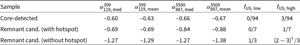
 $^\dagger$ A range is given here, as it is unclear whether MIDAS J225608–341858 (Figure 5c) is ultra-steep at high frequencies.

Figure 7. The high-frequency spectral index  $\alpha_{887}^{5500}$ is plotted against the low-frequency spectral index $\alpha_{119}^{399}$. A third colour bar axis is over-plotted to show the largest angular size in arc-seconds. Solid black line represents a constant spectral index across both frequency ranges. Dashed black line represents a spectral curvature of $\text{SPC}=0.5$. The red dotted and dot-dashed lines represent a $\alpha=-1.2$ spectral index across the low- and high-frequency range, respectively.
Despite the access to high frequencies ( $\nu$ = 5.5 GHz), we find that the selected remnant candidates with hotspots show similar spectral properties to radio galaxies with an active radio core. At low frequencies, remnant candidates with hotspots display spectral indices that are consistent with continuous injection (CI). The high-frequency spectral index does appear to be steeper than for the bulk of remnant candidates with hotspots; however, this is also observed for core-detected radio sources and simply reflects the preferential ageing of higher-energy electrons. No remnant candidates with hotspots display an ultra-steep low-frequency spectral index, and only one such source (e.g. Section 4.2.1) demonstrates a high-frequency ultra-steep spectral index. Regarding these remnant candidates with non ultra-steep spectra, their position on the $\alpha-\alpha$ plot can be explained if these are young, recently switched off remnants. However, their spectral properties can just as easily be explained, if these are active radio galaxies in which the radio core is below the GLASS detection limit. We cannot rule out either of these possibilities based on their spectra alone, and as such they must remain as remnant candidates. We note that Mahatma et al. (Reference Mahatma2018) also report on a large overlap in the observed spectral index (150 MHz–1.4 GHz) between their active and candidate remnant radio galaxies. Only one of their remnant candidates display hotspots at 6 GHz with the VLA telescope, meaning it is not necessarily only the remnant candidates with hotspots which display similar spectral indices as active radio galaxies. A great example of this is the remnant radio galaxy Blob 1 identified by Brienza et al. (Reference Brienza2016).
We also find a small fraction (3/94) of core-detected radio sources which demonstrate an ultra-steep spectral index. The angular size of these sources is well below the largest angular scale that GLASS can recover at 5.5 GHz, suggesting the curvature is genuine. This tells us that ultra-steep selection will not only select radio galaxies in which the AGN has switched off; however, it is interesting to note these sources also do not display GLASS hotspots. It is possible these sources represent restarted radio galaxies in which the ‘core’ represents a newly restarted jet.
Unsurprisingly, we find that the remnant candidates without hotspots also display steeper spectra than those with hotspots. The absence of compact features in their morphologies implies a lack of recent jet activity and is supported by their ultra-steep spectra which implies significant spectral ageing within the lobes. Our low fraction of ultra-steep-spectrum remnant candidates echoes the result of Brienza et al. (Reference Brienza2016) who discuss the bias of preferentially selecting aged remnant radio galaxies via their ultra-steep spectra.
Table 6. Derived distribution averages from Section 5.1.3. The number of radio sources included in each category are denoted by N. The redshift, z, radio power, P, and largest linear size (LLS) are presented. The subscripts med and mean refer to the median and mean values. In the upper half of the table, we consider the entire sample of 104 radio sources. In the lower half, we consider only those with spectroscopic redshifts.
 $^\dagger$ Including the 14 core-detected radio galaxies with $z\geq1$ lower limits.
5.1.3. Power-size distribution
We investigate the sample distribution in redshift, total radio power, and largest linear size (LLS), given the host galaxy identifications. We stress that many of the selected remnant candidates have uncertain host galaxy associations, presenting a major challenge in analysing their rest-frame properties. An additional uncertainty comes from the photometric redshifts, which make up  $60/104$ (57%) of the sample. In addition, 14 active radio galaxies do not have an optical identification, meaning photometric redshift estimates cannot be attained. If we assume their host galaxies are at least $10^{10.6}\textit{M}_{\odot}$, for example, the lowest stellar mass reported by Best et al. (Reference Best, Kauffmann, Heckman, Brinchmann, Charlot and Ivezić2005) to host a radio-loud AGN, we can apply the $K-z$ relation (e.g. see Longair & Lilly Reference Longair and Lilly1984, Rocca-Volmerange et al. Reference Rocca-Volmerange, Le Borgne, De Breuck, Fioc and Moy2004) to estimate the lowest redshift for which a $10^{10.6}\textit{M}_{\odot}$ galaxy will be undetected below the VIKING $K_s$ band AB magnitude limit (Section 2.2.1). This suggests that the host galaxies of the 14 unidentified radio galaxies must be above $z = 1$. The caveat here is that Best et al. (Reference Best, Kauffmann, Heckman, Brinchmann, Charlot and Ivezić2005) investigate local ( $z\leq0.3$) radio-loud AGN samples, whereas here we are assuming higher redshift. Figure 1 of Smolčić et al. (Reference Smolčić2017) shows a hint of a decline in stellar mass with redshift; however, our assumption of the minimum stellar mass seems valid up to $z\sim1$. For each radio source, we calculate the total radio power following: $P= 4\pi S D_L^2(1+z)^{-\alpha - 1}$, where $D_L$ is the luminosity distance. For the 14 radio galaxies without optical identifications, the radio power is calculated assuming $z\geq1$. Our results are presented in Table 6 and Figure 8.

Figure 8. 216-MHz radio power against the largest linear size. Core-detected radio sources (blue markers), remnant candidates with hotspots (orange markers), and remnant candidates without hotspots (red markers) are displayed. Circular and square markers are used to denote spectroscopic and photometric redshifts, respectively. Lower limits on the 14 radio sources without host identifications are denoted by green arrows. Plotted also are the largest linear sizes that would result in a 5 $\sigma$ detection at 216 MHz at $z=0.3$ (black) and $z=1$ (red). Limits are calculated assuming a uniform brightness ellipse, and a lobe axis ratio of 2.5 (solid line) and 1.5 (dashed line). Aged remnants often display low axis ratios, for example, MIDAS J225522 –341807 (Section 4.1.1).
Assuming radio lobes continue expanding once the jets switch off, which at least appears to be the case for FR-II radio galaxies as shown by Godfrey et al. (Reference Godfrey, Morganti and Brienza2017), an expectation of this is for remnants to display larger physical sizes with respect to their active radio galaxy progenitors. Interestingly, our results suggest that the LLSs of core-detected radio galaxies and remnant candidates are similar. This may be explained by the observational bias against remnant radio galaxies of large linear size; such sources will preferentially fall below a fixed detection limit due to their lower surface brightness profiles. Since the linear size and age of a radio galaxy are correlated, for a fixed jet power and environment, it is not unreasonable to suggest that these ‘missing’ remnants also correspond to older remnant radio galaxies, which in turn would imply our sample predominately comprises of young remnants (see also Mahatma et al. Reference Mahatma2018). If so, this result is consistent with the low fraction of ultra-steep remnants discussed in in Section 5.1.2. We do, however, caution this analysis since seven remnant candidates have ambiguous host galaxy associations, as well as the uncertainties surrounding the photometric redshift estimates.
We instead consider the sample of 28 spectroscopically confirmed radio galaxies to see whether we can draw the same conclusions as above. Within this ‘spectroscopic sample’, we can be confident not only of the sample redshifts, but also of the three remnant candidates (e.g. see Section 4.1.2, 4.2.1, and 4.2.5) which have unambiguous host galaxy associations, meaning we can be confident of their positions on the power-size diagram. As demonstrated in Figure 8, the absence of remnant radio galaxies of large linear size becomes quite clear in the ‘spectroscopic sample’ and is consistent with the previously discussed conclusions. Our limiting factor here is the small sample size; however, this will be addressed in future work where we can expect a factor  $\sim6$ increase in the sample size of radio galaxies in GAMA 23. The additional benefit here will be the GAMA 23 group catalogue, which provides group/cluster associations for galaxies with spectroscopic redshifts, as well as virial estimates for the group mass. This will allow us to begin decomposing the degeneracy between radio power, linear size, and environment.
Table 7. Remnant fractions constrained by previous authors. Each column, in ascending order, represents the cited study, the sky coverage over which the sample is compiled, the flux limit across the sample (or the faintest source in the sample), the frequency at which the flux cut is made, the angular size cut of the sample, the number of radio galaxies within the sample, and the resulting remnant fraction. References. (1) Saripalli et al. (Reference Saripalli, Subrahmanyan, Thorat, Ekers, Hunstead, Johnston and Sadler2012), (2) Brienza et al. (Reference Brienza2017) and Jurlin et al. (Reference Jurlin2020), (3) Mahatma et al. (Reference Mahatma2018), (4) This work.
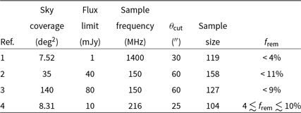
5.2. Constraining a remnant fraction
5.2.1. Remnant fraction upper limit
The fraction of remnant radio galaxy candidates identified in this work provides an upper limit to the genuine fraction of remnant radio galaxies,  $f_\mathrm{rem}$, present within this sample. Of 104 radio galaxies, 10 are identified as remnant radio galaxy candidates, resulting in a $f_\mathrm{rem}\approx10\%$ upper limit on the remnant fraction. Saripalli et al. (Reference Saripalli, Subrahmanyan, Thorat, Ekers, Hunstead, Johnston and Sadler2012), Brienza et al. (Reference Brienza2017), and Mahatma et al. (Reference Mahatma2018) each constrain a remnant fraction from radio observation and their results are presented in Table 7. At face value, the remnant fraction obtained in this work is consistent with that of Brienza et al. (Reference Brienza2017) and Mahatma et al. (Reference Mahatma2018) and shows a considerable increase over the fraction constrained by Saripalli et al. (Reference Saripalli, Subrahmanyan, Thorat, Ekers, Hunstead, Johnston and Sadler2012). The apparent inconsistency with Saripalli et al. (Reference Saripalli, Subrahmanyan, Thorat, Ekers, Hunstead, Johnston and Sadler2012) may very well be a result of their selection. Their sample was selected at 1.4 GHz, where ultra-steep remnants may potentially be missed, and they also excluded sources without a radio core but hotspots still present within the lobes. It is interesting to note that despite the difference in the flux limit and angular size cut compared to the samples complied by Mahatma et al. (Reference Mahatma2018), Brienza et al. (Reference Brienza2017), and Jurlin et al. (Reference Jurlin2020), the upper limits on the remnant fraction appear consistent. Shabala et al. (Reference Shabala2020) show that the remnant fraction predicted by constant-age models, for example, those in which the jets are active for a constant duration, is highly sensitive to observable constraints, for example, the flux and angular size limit. On the other hand, the remnant fraction predicted by power law age models, for example, those in which the duration of the active phase is power law-distributed, shows little dependence on observable parameters. It is therefore possible that the similarity in remnant fractions implies a preference towards power law age models that describe AGN jet activity, although this needs to be pursued in more detailed future work.

Figure 9. Modelled integrated spectrum of MIDAS J225337–344745. Figure 9a models the spectrum assuming a continuous injection model (CI). Figure 9b models the spectrum assuming a continuous injection model with an ‘off’ component, encoding a jet switch-off (CI off). In each model, a 2 $\sigma$ uncertainty envelope is represented by the violet shaded region. As discussed in Section 5.3, the model uncertainties take into account only the uncertainties on the flux density measurements and do not reflect the underlying uncertainties due to an inhomogeneous magnetic field. For reference, a best fit to the data using single power law model is represented by a blue line.
5.2.2. Remnant candidates without hotspots
As presented in Section 4, the lobes of seven remnant candidates display compact emitting regions in GLASS, potentially indicating a hotspot formed by an active jet. As discussed in Sections 5.1.1 and 5.1.2, these sources could be interpreted either as recently switched off remnants, or, active radio galaxies with unidentified radio cores. We thus propose a lower limit to the remnant fraction, by considering the limiting case where each remnant candidate with a hotspot is an active radio galaxy. This would suggest a  $f_{\mathrm{rem}}=4/104$ ( $\approx4\%$) lower limit on the remnant fraction, consistent with the value reported by Saripalli et al. (Reference Saripalli, Subrahmanyan, Thorat, Ekers, Hunstead, Johnston and Sadler2012). As discussed in Section 5.3, an appreciable fraction of genuine remnants with hotspots can potentially be expected.
5.3. Evolutionary history of MIDAS J225337–344745
A particularly interesting source to examine is MIDAS J225337–344745, which as mentioned in Section 4.2.1, demonstrates two seemingly contradictory features: the higher-frequency ultra-steep ( $\alpha<-1.52$) spectrum of the lobes, suggesting energy losses consistent with an aged remnant radio galaxy, and the compact 5.5-GHz emitting regions in GLASS, which may in turn suggest current or recent energy injection. It is unclear whether these are genuine hotspots; the north-eastern lobe is detected just above the noise level and thus demonstrates many ‘hotspot-like’ features. A singular, bright ‘hotspot’ is evident in the south-western lobe; however, the emitting region is clearly resolved at a physical resolution of $7\times14$ kpc (the physical resolution of GLASS 5.5 at $z=0.213$), and so it is unclear whether this ‘hotspot’ is formed by an active jet, or, whether it is the expanding hotspot of a previously active jet. It is also possible that the compact emitting region is a combination of the lobe and hotspot. Fortunately, the radio continuum spectrum appears to preserve the original spectrum at low frequencies, while also encoding the energy losses evident at higher frequencies. This allows us to model and parameterise the spectrum in terms of physically meaningful parameters, allowing us to probe the energetics along with the dynamics. Our ultimate objective here is to determine whether the compact emitting regions can be expected within a remnant radio galaxy. Our analysis is laid out as follows.
We model the radio source using the Radio AGN in Semi-analytic Environments (RAiSE) code which considers, amongst other things: (i) the evolution of the magnetic field strength; (ii) the adiabatic losses contributing to the radio luminosity evolution of the lobes; and (iii) the Rayleigh–Taylor mixing of the plasma contained within the remnant lobes. These processes are described by the dynamical (Turner & Shabala Reference Turner and Shabala2015) and synchrotron emissivity (Turner, Shabala, & Krause Reference Turner, Shabala and Krause2018b) models for lobes FR-II radio lobes, which follow the CI model (Kardashev Reference Kardashev1962; Pacholczyk Reference Pacholczyk1970; Jaffe & Perola Reference Jaffe and Perola1973). The remnant spectrum follows the CI ‘off’ model (CI-off or KGJP model; Komissarov & Gubanov Reference Komissarov and Gubanov1994), which Turner (Reference Turner2018) parameterise with two break frequencies. A jet power Q  $=10^{38.1}$ W, magnetic field strength $B=1.08$ nT, and total source age $\tau=71$ Myr are constrained by the method of Turner et al. (Reference Turner, Shabala and Krause2018b). The synchrotron spectrum is modelled by the method of Turner (Reference Turner2018) which, provided sufficient spectral sampling, allows the injection index $\alpha_{\mathrm{inj}}$, break frequency $\nu_b$, and quiescent fractionFootnote m T to be uniquely constrained. Our results are shown in Figure 9. Both models constrain an injection index that is consistent within their typically observed range of $-1.0<\alpha_{\mathrm{inj}}< -0.5$ (see Table 8). The discrepancy between the modelling becomes evident at the highest frequencies, for which the CI model begins to over-predict the integrated flux density. On the other hand, the CI-off model is able to comfortably reproduce the observed SPC. We calculate a reduced chi $^2$ ( $\chi^2_{\mathrm{red}}$) for each model, and a $\Delta$ BIC $=2.1$ (by BIC $_{\mathrm{CI}}$ – BIC $_{\mathrm{CI-off}}$) which demonstrates a preference towards the CI-off model (see Table 8). Although the distinction between the two models is ultimately driven by the 9-GHz measurement, CI-off provides a better model of the observed spectrum suggesting these are remnant lobes. Modelling the spectrum as a remnant suggests the source spends approximately 21 Myr in a remnant phase.
Table 8. Summarised properties of MIDAS J225337–344745 spectral modelling (Section 5.3). A reduced chi-squared ( $\chi^2_{\text{red}}$) is provided to assess the quality of fit. The injection index $\alpha_{\text{inj}}$, observed frame break frequency $\nu_b$, and quiescent fraction T are presented for the fitted continuous injection (CI) and continuous injection-off CI-off models. We quote a $\Delta$BIC calculated between the two models.

Turner et al. (Reference Turner, Shabala and Krause2018b) showed that the CI model provides a statistically significant fit to the broad frequency radio spectra of over 86 % of FR-IIs in the Mullin et al. (Reference Mullin, Riley and Hardcastle2008) sample of 3C sources (typically 12 measurements between 0.01 and 10 GHz from Laing & Peacock Reference Laing and Peacock1980; but see Harwood Reference Harwood2017). Further, despite the non-physical CI model assumption of time-invariant magnetic fields, Turner et al. (Reference Turner, Shabala and Krause2018b) find that CI model is an excellent fit to the simulated spectra of lobed FR-II which do consider magnetic field evolution and are able to recover the source dynamical age.
As a final sanity check on the duration of the remnant phase fitted above (by the integrated CI-off model), we constrain the age of the most recently accelerated electron populations which we assume are located near the ‘hotspots’. We convolve the radio observations at 399, 887, and 5.5 GHz images to a common 11 arcsec circular resolution and measure the integrated flux density within an aperture centred at the southern ‘hotspot’. We fit the spectrum with a Tribble JP model assuming the magnetic field derived previously in our RAiSE modelling. We arrive at a remnant age of  $t_{\mathrm{off}}=13_{-4}^{+8}$ Myr, consistent with the $t_{\mathrm{off}}\approx21$ Myr derived from the integrated CI-off model. We stress that the observations are not properly (u,v) matched and thus are not necessarily seeing the same radio emission, for example, at 5.5 GHz, the flux density is likely underestimated due to resolving out the extended radio emission. We leave a more detailed analysis of this source to future work.
Next, we model the hotspot to better understand its typical fading timescale. We model a ‘MIDAS J225337–344745 like’ radio galaxy, meaning we adopt the same values for the jet power, active age, lobe axis ratio, energy injection index, and equipartition factor. By the method of Turner et al. (Reference Turner, Rogers, Shabala and Krause2018a), we forward model the 5.5-GHz lobe spatial emissivity (without the hotspot) and convolve the output map with the GLASS 5.5 synthesised beam. We consider the GLASS 5.5 beam with the largest integrated flux (e.g. the maximum peak flux density), as this ultimately determines whether the youngest emitting regions of the lobes are detected. The hotspot is modelled assuming a JP spectrum (Jaffe & Perola Reference Jaffe and Perola1973) for the same initial properties as the lobe but for an increased magnetic field strength. Cygnus A displays a factor 5 increase in the hotspot magnetic field strength, in comparison to that of the lobes (Carilli & Barthel Reference Carilli and Barthel1996). We make the same assumption for MIDAS J225337–344745; however, also consider a case where the hotspot magnetic field strength is a factor 10 greater than the lobes. We also assume the same ratio of hotspot to lobe volume as that measured in Cygnus A; this only shifts the spectrum along the log-frequency log-luminosity plane and does not influence the spectral shape (i.e. the slope). Our results are presented in Figure 10. As expected, the hotspot fades rapidly once injection switches off. Bright radio emission from the hotspot is driven by the freshly injected electrons which have a short lifetime at high frequencies due to the strong magnetic field. Despite the hotspot fading rapidly, its fading timescale is non-negligible when compared to the characteristic active and remnant ages. It is not unreasonable to suggest that recently switched off remnants may still display hotspots, and that some of the selected remnant candidates with hotspots (Section 5.2.2) may indeed be such cases. The main result of Figure 10 is that the hotspots of a recently switched off jet should not be visible in MIDAS J225337–344745, assuming a  $t_{\mathrm{off}}\approx21$ Myr remnant phase. At the implied age of the remnant, the modelled emitting regions of the lobes range between 100 and 150 kpc in size. This is consistent with the observed emitting regions in GLASS, which demonstrate a projected linear size of $\sim96$ kpc. This indicates that the bright features in GLASS are entirely consistent with the youngest plasma regions and are not necessarily the hotspots of an active jet.

Figure 10. A ‘MIDAS J225337–344745’-type remnant radio galaxy is modelled by assuming a jet power  $Q=10^{38.1}$ W, an injection energy index of $s=2.1$, an equipartition factor of $B/B_{\text{eq}}=0.22$, and a total source age of 71 Myr of which 50 Myr is spent in an active phase, and a further 21 Myr is spent as a remnant. The shaded blue bar corresponds to the time during which the source is active, after which the jets are switched off and the hotspots/lobes begin to fade. The evolution of the synchrotron emission from the lobes (solid black tracks) and the hotspots (dashed tracks) are shown as a function of the total source age. The assumption that the hotspot magnetic field strength is a factor 5 greater than the lobes (coloured in orange) comes from Cygnus A; however, we also assume a factor 10 increase in the hotspot magnetic field strength (coloured in red) to consider shorter fading timescales. We explore this in terms of the peak flux density, as this ultimately decides whether the emitting regions are detected in observations. The vertical drop in the flux density tracks reflects the depletion of electrons capable of producing emission at 5.5 GHz. As expected, the synchrotron emission evolves faster in the hotspot; however, their fading timescale is non-negligible in comparison to that of the lobes.
As such, the interpretation of this source is challenging for the following reasons. Modelling the spectrum suggests these are the lobes of a remnant radio galaxy. While hotspots will remain visible for a non-negligible period of time after injection is switched off, they should not be visible in this source assuming the remnant age is correct. The two pieces of evidence are consistent with one another if the bright GLASS features are just the youngest emitting regions of the lobes. If we alternatively assume MIDAS J225337–344745 is an active source, the RAiSE modelling of Turner et al. (Reference Turner, Shabala and Krause2018b) finds a comparable age ( $\tau = 100\rm\: Myr$) to the remnant case but a substantially lower jet power of $Q=10^{36.7}\rm\: W$ is required to match the relatively low observed flux density. This jet power is typically associated with an FR-I morphology for the known host galaxy mass (e.g. Ledlow Reference Ledlow1994; Best Reference Best2009), potentially resulting in a broad flare point rather than compact hotspots at the end of a jet. This morphology may explain the large spatial extent of the GLASS 5.5 GHz observations; however, it does not resolve the discrepant SPC.
Finally, the result presented in Figure 10 makes a rather interesting prediction for the observed properties of genuine remnants. As discussed in Section 5.2, the upper limit on the remnant fraction is  $f_{\mathrm{rem}}\approx10\%$. For a characteristic active lifetime of $\sim100$ Myr, our observed remnant fraction would thus suggest an observable remnant phase lasting $\sim10$ Myr. The modelling of a ‘MIDAS J225337–344745-like’ radio galaxy shows that the hotspot can persist for at least several Myr before fading out completely. As such, we can expect an appreciable fraction of remnants to still display hotspots.
6. Conclusions
Within a subregion of 8.31 deg $^2$ of the GAMA 23 field, we have compiled a sample consisting of 104 extended, low-frequency selected (216 MHz) radio galaxies. Using the 5.5- and 9.5-GHz GLASS survey, we have adopted the ‘absent radio core’ criterion to search for remnant radio galaxy candidates. Our conclusions are summarised as follows:
We identify 10 new remnant radio galaxy candidates, thereby constraining an
$f_{\mathrm{rem}} \leq 10\%$ upper limit on the fraction of radio galaxies with quiescent AGN. Our upper limit is consistent with that proposed by previous authors and suggests that remnants must have a short observable lifetime.Seven remnant candidates show compact emitting regions in GLASS, an observation that can only be explained if the jets have recently switched off. A much smaller fraction (3/10) show relaxed, hotspot-less lobes, and only one displays an ultra-steep-spectrum across the entire frequency range. This implies remnants are detected soon after switching off, suggesting a rapid fading during the remnant phase.
The small fraction of ultra-steep (
$\alpha<-1.2$) remnants is likely a result of the oldest remnant lobes escaping detection due to their expansion.At present, the upper limits placed on the remnant core prominence are too weak to confidently rule out the presence of AGN activity. Those with compact hotspots and a non-ultra-steep-spectrum must therefore retain their remnant candidate classification. Considering the limiting case in which all these are active radio galaxies, we would expect a
$f_{\mathrm{rem}}\approx4\%$ remnant fraction.MIDAS J225337–344745 represents an interesting object for future study. Modelling the integrated lobe spectrum shows consistency with a remnant radio galaxy. We find that although the hotspot has a non-negligible fading timescale, we do not expect to see hotspots in this source.
By modelling the synchrotron spectrum arising from a ‘MIDAS J225337 – 344745-like’ hotspot, we show that the hotspot can persist for
$5-10$ Myr at 5.5 GHz after the jets switch off. This would imply that the presence of a hotspot in radio maps may not necessarily reflect an active jet, and by extension we can expect an appreciable fraction of genuine remnants to still display hotspots.


Acknowledgements
BQ acknowledges a Doctoral Scholarship and an Australian Government Research Training Programme scholarship administered through Curtin University of Western Australia. NHW is supported by an Australian Research Council Future Fellowship (project number FT190100231) funded by the Australian Government. This scientific work makes use of the Murchison Radio-astronomy Observatory, operated by CSIRO. We acknowledge the Wajarri Yamatji people as the traditional owners of the Observatory site. Support for the operation of the MWA is provided by the Australian Government (NCRIS), under a contract to Curtin University administered by Astronomy Australia Limited. We acknowledge the Pawsey Supercomputing Centre which is supported by the Western Australian and Australian Governments. The Australian SKA Pathfinder is part of the Australia Telescope National Facility which is managed by CSIRO. Operation of ASKAP is funded by the Australian Government with support from the National Collaborative Research Infrastructure Strategy. The Australia Telescope Compact Array is part of the Australia Telescope National Facility which is funded by the Australian Government for operation as a National Facility managed by CSIRO. We thank the staff of the GMRT that made these observations possible. GMRT is run by the National Centre for Radio Astrophysics of the Tata Institute of Fundamental Research. CHIC acknowledges the support of the Department of Atomic Energy, Government of India, under the project 12-R&D-TFR-5.02-0700. SW acknowledges the financial assistance of the South African Radio Astronomy Observatory (SARAO) towards this research is hereby acknowledged (www.ska.ac.za). IP acknowledges support from INAF under the SKA/CTA PRIN ‘FORECaST’ and the PRIN MAIN STEAM ‘SAuROS’ projects. The National Radio Astronomy Observatory is a facility of the National Science Foundation operated under cooperative agreement by Associated Universities, Inc. H.A. benefited from grant CIIC 90/2020 of Universidad de Guanajuato, Mexico. We acknowledge the work and support of the developers of the following Python packages: Astropy (Astropy Collaboration et al. Reference Astropy2013; Price-Whelan et al. Reference Price-Whelan2018) and Numpy (van der Walt, Colbert, & Varoquaux Reference van der Walt, Colbert and Varoquaux2011). We also made extensive use of the visualisation and analysis packages DS9Footnote n and Topcat (Taylor Reference Taylor2005). We thank an anonymous referee for their insightful comments that have improved the manuscript. This work was compiled in the very useful free online editor Overleaf.
Supplementary Material
To view supplementary material for this article, please visit https://doi.org/10.1017/pasa.2020.49
Appendix
Table A1. Column descriptions corresponding to the supplementary electronic table. The MIDAS_Name is derived using the MIDAS_RA and MIDAS_Dec columns. Entries without a GAMA_IAUID, mag_Ks, or NED_Object_Name are assigned a value of ’ $-99$’. Hotspots (L1) and Hotspots (L2) refer to the number of GLASS hotspots found in each lobe, where L1 and L2 refer to the lobe and counter-lobe. We define L1 as having the smaller position angle measured in a counter-clockwise direction from the North.


