


1. Introduction
All-sky imaging is a very powerful and unique feature of low-frequency interferometers operating below 400 MHz, where the individual antennas can see the entire hemisphere. Several all-sky monitoring systems have been implemented in the Northern Hemisphere. The Amsterdam-ASTRON Radio Transient Facility And Analysis Centre (AARTFAAC; Prasad et al. Reference Prasad2016) is a parallel transient detection instrument operating as a subsystem of the LOw Frequency ARray (LOFAR; van Haarlem et al. Reference van Haarlem2013) observing at frequencies between 10 and 90 MHz. Similarly, the Long Wavelength Array (LWA; Ellingson et al. Reference Ellingson2013) observes in the 10–88 MHz frequency band.
These facilities are used for monitoring large swaths of the sky for transients. They have reported multiple results related to astrophysical transients ranging from detections of local Jovian bursts (Imai et al. Reference Imai2016), extremely bright pulses from pulsars such as PSR B0950+08 (Kuiack et al. Reference Kuiack, Wijers, Rowlinson, Shulevski, Huizinga, Molenaar and Prasad2020c), flare stars (Davis, Taylor, & Dowell Reference Davis, Taylor and Dowell2020), meteor radio afterglows (Obenberger et al. Reference Obenberger2014b), limits on prompt emission from gamma-ray bursts (Obenberger et al. Reference Obenberger2014a; Anderson et al. Reference Anderson2018), to detections of short-timescale transients that are of yet unknown origin (Varghese et al. Reference Varghese, Obenberger, Dowell and Taylor2019; Kuiack et al. Reference Kuiack, Wijers, Shulevski and Rowlinson2020a, 2020b). Furthermore, the all-sky imaging searches have resulted in very stringent limits on transient surface densities (e.g. Anderson et al. Reference Anderson2019; Kuiack et al. Reference Kuiack, Wijers, Shulevski, Rowlinson, Huizinga, Molenaar and Prasad2020b). Extremely interesting detections already obtained by all-sky monitoring systems prove that these systems are powerful transient-instruments complementing wide-field and all-sky telescopes using other electromagnetic wavelengths or messengers (e.g. neutrino telescopes, gravitational waves detectors, etc.) and have a potential of generating high impact scientific results. Especially, in the light of the recent detections of fast radio bursts (FRBs) below 400 MHz, such as the low-frequency detections of repeating FRB 20180916B discovered by Canadian Hydrogen Intensity Mapping Experiment (CHIME/FRB CHIME/FRB Collaboration et al. 2018, 2019) and recently detected by LOFAR at 110–188 MHz (Pleunis et al. Reference Pleunis2020; Pastor-Marazuela et al. Reference Pastor-Marazuela2020) and Sardinia Radio Telescope (Pilia et al. Reference Pilia2020) or FRB 20200125A discovered by Green Bank Telescope at 350 MHz (Parent et al. Reference Parent2020). Although the Northern Hemisphere systems cover some fractions of the southern sky, to date, no dedicated system capable of continuous monitoring of the entire Southern Hemisphere has existed.
We present the first all-sky transient monitoring facility in the Southern Hemisphere realised on the prototype stations of the low-frequency component of the Square Kilometre Array (SKA-Low; Dewdney et al. Reference Dewdney, Hall, Schilizzi and Lazio2009).Footnote a This system takes advantage of the two prototype stations, the Engineering Development Array 2 (EDA2; Wayth et al., in preparation) and Aperture Array Verification System 2 (AAVS2; van Es et al. Reference van Es2020; Davidson et al. Reference Davidson2020a), which were deployed at the MRO in 2019 to verify the technology and performance of different antenna designs against the SKA-Low requirements. These stations can observe in the same frequency band (50–350 MHz) as intended for the full SKA-Low. More importantly to the presented project, they can be operated as standalone interferometers and form all-sky images from correlation products (visibilities) of all antenna pairs within the station. These images can then be searched for transients either in real-time or off-line.
Real-time all-sky imaging has recently been implemented, and multiple long commissioning observations were performed with one or both stations observing in parallel in the same or different frequency bands. Although the most common transient candidates are due to radio-frequency interference (RFI, due to transmissions or reflections from aircraft, satellites, or meteors), similar to those reported by Tingay et al. (Reference Tingay, Sokolowski, Wayth and Ung2020) in the FM frequency band (98.44 MHz), several transients of confirmed astrophysical origin have also been identified. The brightest and most interesting among them were extremely bright transients ( $\sim$
150 Jy beam–1, i.e. fluence
$\sim$
150 Jy beam–1, i.e. fluence $\sim$
300 kJy beam–1 ms) from the pulsar PSR B0950+08. The pulsar PSR B0950+08 is a relatively long-known pulsar first reported as Cambridge Pulsed source CP0950 by Pilkington et al. (Reference Pilkington, Hewish, Bell and Cole1968). Nevertheless, it has recently been generating a lot of attention due to its exceptional brightness; its high variability; the detections of its extremely bright events by Kuiack et al. (Reference Kuiack, Wijers, Rowlinson, Shulevski, Huizinga, Molenaar and Prasad2020c) (potentially similar to the giant pulses produced by the Crab pulsar); the recent confirmation of the surrounding pulsar wind nebula (Ruan et al. Reference Ruan, Taylor, Dowell, Stovall, Schinzel and Demorest2020); and brightness enabling studies of the substructure of individual pulses in high-time resolution (McSweeney et al. Reference McSweeney2020).
$\sim$
300 kJy beam–1 ms) from the pulsar PSR B0950+08. The pulsar PSR B0950+08 is a relatively long-known pulsar first reported as Cambridge Pulsed source CP0950 by Pilkington et al. (Reference Pilkington, Hewish, Bell and Cole1968). Nevertheless, it has recently been generating a lot of attention due to its exceptional brightness; its high variability; the detections of its extremely bright events by Kuiack et al. (Reference Kuiack, Wijers, Rowlinson, Shulevski, Huizinga, Molenaar and Prasad2020c) (potentially similar to the giant pulses produced by the Crab pulsar); the recent confirmation of the surrounding pulsar wind nebula (Ruan et al. Reference Ruan, Taylor, Dowell, Stovall, Schinzel and Demorest2020); and brightness enabling studies of the substructure of individual pulses in high-time resolution (McSweeney et al. Reference McSweeney2020).
The presented transient detection system is at a very early development stage and many further improvements are planned, such as automatic classification capability to enable efficient excision of RFI and other non-astrophysical transients. However, the excision of RFI will be significantly improved with the planned increase in bandwidth (to $\sim$
50 MHz) and time resolution to tens of milliseconds.
$\sim$
50 MHz) and time resolution to tens of milliseconds.
This paper is organised as follows. In Section 2, we present the SKA-Low stations which were used to develop the all-sky transient monitoring system. In Section 3, we describe the data acquisition mode and observations used in this paper. In Section 4, we present the all-sky imaging system and all stages of data pre-processing, calibration, and imaging leading to all-sky images used as a basis for the transient monitoring. In Section 5, we present the all-sky transient monitoring system and the early version of transient identification and classification. In Section 6, we discuss the preliminary results obtained with this system ranging from RFI-related events to transients from astrophysical objects, especially the extreme activity of the pulsar PSR B0950+08. In Section 7, we describe low-frequency upper limits on the flux density of two FRBs, and in Section 8 a preliminary upper limit on transient surface density is discussed. In Section 9, we outline potential other applications of the real-time imaging pipeline. Finally, a summary of this work is provided in Section 10, and in Section 11 we discuss future improvements in the system.
2. SKA-Low prototype stations
The SKA-Low will be a low-frequency (50–350 MHz) radio-telescope of an unprecedented collecting area and sensitivity. It will consist of 512 stations each composed of 256 dual-polarised antennas. In 2016, the first full-scale (256 dual-polarised antennas) prototype SKA-Low station, the Engineering Development Array 1 (EDA1; Wayth et al. Reference Wayth2017) was deployed at the MRO. It was composed of 256 dual-polarisation bow-tie dipoles of the same design as used in the Murchison Widefield Array (MWA; Tingay et al. Reference Tingay2013; Wayth et al. Reference Wayth2018) arranged in pseudo-random SKA-Low layout within a 35-m diameter. It was deployed in order to assess applicability of the MWA-like technology (bow-tie dipoles and analogue beamforming) for the SKA-Low and as a reference for the Aperture Array Verification System 1 (AAVS1; Bentham et al. submitted), which was deployed at the MRO in 2017.
In 2019, based on these experiences, two further prototype stations were deployed at the MRO. They use the same signal chain technology and antenna layout as their predecessor AAVS1 station, but the antenna designs in both stations are different. The left panel of Figure 1 shows the EDA2 station, which as its predecessor (EDA1) consists of 256 MWA bow-tie dipoles, while the AAVS2 station shown in the right panel of Figure 1 is composed of the SKALA4.1 antennas (Bolli et al. Reference Bolli2020, de Lera Acedo, Pienaar, & Fagnoni Reference de Lera Acedo, Pienaar and Fagnoni2018). The diameter of the AAVS2 station (maximum distance between antenna centres $\approx$
38 m) has been increased by about 10% with respect to the other stations (EDA1, EDA2, and AAVS1).
$\approx$
38 m) has been increased by about 10% with respect to the other stations (EDA1, EDA2, and AAVS1).
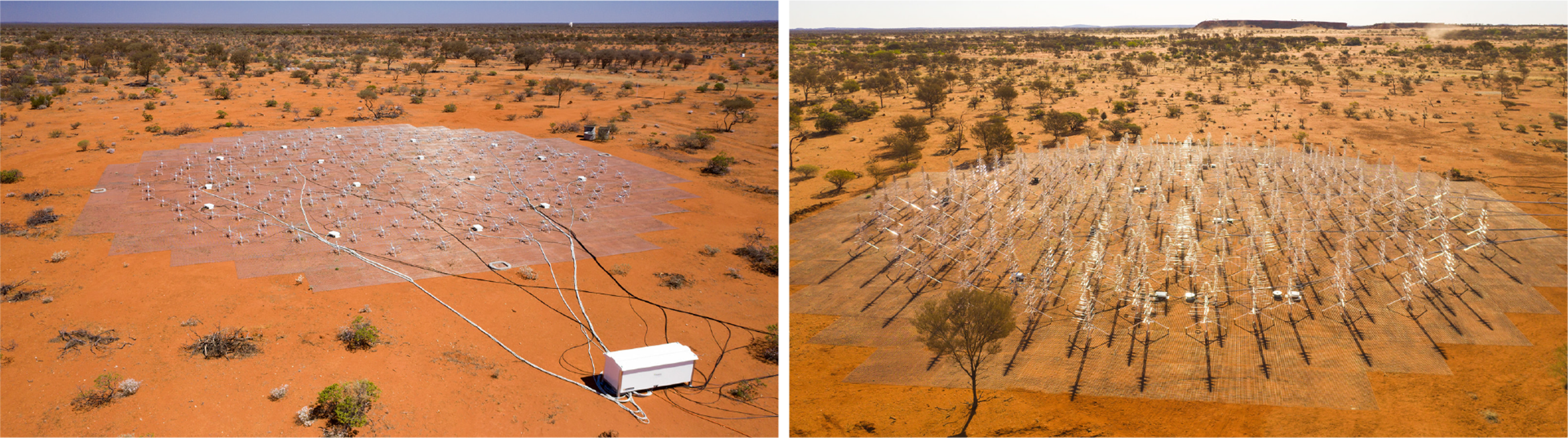
Figure 1. An aerial view of the SKA-Low prototype stations EDA2 composed of 256 MWA bow-tie dipoles (left image) and AAVS2 composed of 256 SKALA4.1 antennas (right image), which were used for this paper.
The analogue signals from individual antennas (X and Y polarisations) are converted to optical signals near the antennas and transported over the 5.5 km fibre to the central processing facility. The EDA2 and AAVS2 both use tile processing modules (TPM; Naldi et al. Reference Naldi2017) to digitise incoming signals. The TPM is a 32-input signal processing board designed for SKA-Low. Each TPM digitises 32 inputs at 800 M samples s–1 with 8-bit resolution, for a total ingest of 25.6 GB s–1 per board (409.6 GB s–1 per station).
Steam-processing firmware running on the TPM boards coarsely channelises the incoming voltage streams into 512 channels of width $\approx$
0.926 MHz; this firmware is detailed in Comoretto et al. (Reference Comoretto2017). The EDA2 and AAVS2 are connected by high-speed Ethernet to a software correlator running on commercial-off-the-shelf computer hardware with both stations using exactly the same rack-mounted Dell servers each with two Intel Xeon Gold 6226 2.7 GHz, 192 GB RAM, 64 TB of SSD hard-drives in RAID5 for the data, two 240 GB solid-state drives in RAID1 for the operating system, NVIDIA Tesla V100 16GB GPU, and one Mellanox ConnectX-5 dual port 40/100 Gb Ethernet card. We use a custom Ethernet packet capture code and the xGPU software correlator (Clark, La Plante, & Greenhill Reference Clark, La Plante and Greenhill2011) to perform cross-correlation with all 256 inputs in real time.
$\approx$
0.926 MHz; this firmware is detailed in Comoretto et al. (Reference Comoretto2017). The EDA2 and AAVS2 are connected by high-speed Ethernet to a software correlator running on commercial-off-the-shelf computer hardware with both stations using exactly the same rack-mounted Dell servers each with two Intel Xeon Gold 6226 2.7 GHz, 192 GB RAM, 64 TB of SSD hard-drives in RAID5 for the data, two 240 GB solid-state drives in RAID1 for the operating system, NVIDIA Tesla V100 16GB GPU, and one Mellanox ConnectX-5 dual port 40/100 Gb Ethernet card. We use a custom Ethernet packet capture code and the xGPU software correlator (Clark, La Plante, & Greenhill Reference Clark, La Plante and Greenhill2011) to perform cross-correlation with all 256 inputs in real time.
Thus, both stations form 256 element, dual-polarisation interferometers that can be used to produce all-sky images with standard interferometric calibration and imaging techniques. The TPMs can also generate real-time station beams to be correlated with other stations, which will be a typical operation mode for the SKA-Low. However, we do not compute inter-station cross correlations for the work presented here. Nevertheless, this functionality may also be used by the presented system to automatically form station beams in the direction of transients identified by the real-time system or provided by external alerts.
3. Observations
Multiple long (typically longer than 24 h) observations have been performed at several frequencies since both stations were fully deployed at the MRO in 2019. A lot of these observations were conducted with both stations collecting correlated data simultaneously at 2 s resolution and single coarse channel of $\approx$
0.926 MHz bandwidth. Presently, the system can collect correlated data in a single coarse channel, which is its main limitation and will be discussed in Section 11. Many nights of observations dedicated to development of the presented system have also been collected and Table 1 contains a summary of the observations used for this paper. All the presented data were collected at frequencies equal or above 159.375 MHz and stations recorded either the same frequency channel or AAVS2 observed at a higher frequency channel than the EDA2.
$\approx$
0.926 MHz bandwidth. Presently, the system can collect correlated data in a single coarse channel, which is its main limitation and will be discussed in Section 11. Many nights of observations dedicated to development of the presented system have also been collected and Table 1 contains a summary of the observations used for this paper. All the presented data were collected at frequencies equal or above 159.375 MHz and stations recorded either the same frequency channel or AAVS2 observed at a higher frequency channel than the EDA2.
Table 1. Number of candidates after the main filtering criteria for 14 analysed nights when both stations were collecting data. For some columns, two numbers are shown for the EDA2 and AAVS2, respectively. The columns ${N}_{\text{eda2}}$
and
${N}_{\text{eda2}}$
and ${N}_{\text{aavs2}}$
are numbers of transients detected in difference images from the EDA2 and AAVS2 stations, respectively.
${N}_{\text{aavs2}}$
are numbers of transients detected in difference images from the EDA2 and AAVS2 stations, respectively. ${N}_{\text{coinc}}$
is the number of candidates after requiring time coincidence, that is, maximum of 2 s or dispersion time corresponding to maximum DM=1 000 pc cm-3 if the stations observed at different frequencies, and spatial coincidence in radius
${N}_{\text{coinc}}$
is the number of candidates after requiring time coincidence, that is, maximum of 2 s or dispersion time corresponding to maximum DM=1 000 pc cm-3 if the stations observed at different frequencies, and spatial coincidence in radius $R_{\rm coinc} = 3.3^\circ$
between both stations.
$R_{\rm coinc} = 3.3^\circ$
between both stations. ${N}_{\text{sat}}$
is the number of candidates matched to satellites in TLE catalogue according to the criteria described in the text.
${N}_{\text{sat}}$
is the number of candidates matched to satellites in TLE catalogue according to the criteria described in the text. ${N}_{\text{acc}}$
is the number of the remaining candidates (excluding the transients associated with PSR B0950+08 shown in the separate column
${N}_{\text{acc}}$
is the number of the remaining candidates (excluding the transients associated with PSR B0950+08 shown in the separate column ${N}_{\text{B0950}}$
), which are potentially of astrophysical origin
${N}_{\text{B0950}}$
), which are potentially of astrophysical origin
aFrequencies are approximated to a first decimal digit with the exact frequencies 159.375, 229.6875, 312.5, and 320.3125 MHz; at these frequencies, the synthesised beam sizes are approximately $2.4^\circ$ $(2.2^\circ)$
,
$(2.2^\circ)$
, $1.7^\circ (1.5^\circ)$
,
$1.7^\circ (1.5^\circ)$
, $1.1^\circ$
, and
$1.1^\circ$
, and $1.2^\circ(1.1^\circ)$
, respectively, where values in brackets are for the AAVS2 station (except 312.5 MHz observed only with AAVS2 station).
$1.2^\circ(1.1^\circ)$
, respectively, where values in brackets are for the AAVS2 station (except 312.5 MHz observed only with AAVS2 station).
bThe number of astrophysical candidates after excluding candidates caused by the PSR B0950+08 pulses.
cThese candidates were discarded upon visual inspection as satellites, planes, or artefacts.
dNumber of candidates which passed visual inspection, but could not be confirmed to be of astrophysical origin.
eMultiple transients from the same position, which is currently under investigation and will be reported in a future publication.
fThe EDA2 was only collecting data for about 3 h, but more AAVS2 data were used for PSR B0950+08 monitoring.
gRejected as a moving object (most likely a satellite) after visual inspection of images.
4. Real-time all-sky imager
4.1. Data pre-processing
The correlation products in $\approx$
2 s resolution are saved in HDF5 format,Footnote b which is envisaged as the data format for the SKA telescope. The system waits for the new HDF5 file to be collected and converts it into the UV FITS file (Greisen Reference Greisen2019) in the native time resolution using the current metadata information, which includes list of flagged antennas, antenna positions, etc. We used auto-correlation spectra to identify and flag antennas with very low power, and antennas which did not calibrate well (i.e. calibration solutions as a function of frequency did not have clear linear form). In the conversion process, the zenith is used as the phase centre, and therefore the resulting images are zenith-centred (Section 4.3). Time averaging is available in the correlator, but the system was always running at the currently highest possible time resolution of 1.96 s. Further processing was performed with the Miriad data processing suite (Sault, Teuben, & Wright Reference Sault, Teuben and Wright1995). In the next step, pre-calculated calibration solutions are applied to the data in UV format (Section 4.2).
$\approx$
2 s resolution are saved in HDF5 format,Footnote b which is envisaged as the data format for the SKA telescope. The system waits for the new HDF5 file to be collected and converts it into the UV FITS file (Greisen Reference Greisen2019) in the native time resolution using the current metadata information, which includes list of flagged antennas, antenna positions, etc. We used auto-correlation spectra to identify and flag antennas with very low power, and antennas which did not calibrate well (i.e. calibration solutions as a function of frequency did not have clear linear form). In the conversion process, the zenith is used as the phase centre, and therefore the resulting images are zenith-centred (Section 4.3). Time averaging is available in the correlator, but the system was always running at the currently highest possible time resolution of 1.96 s. Further processing was performed with the Miriad data processing suite (Sault, Teuben, & Wright Reference Sault, Teuben and Wright1995). In the next step, pre-calculated calibration solutions are applied to the data in UV format (Section 4.2).
4.2. Calibration
The full band calibration scheme for the stations is an extension of the procedure described by Bentham et al. (submitted) and it will be briefly summarised here. Due to current bandwidth limitations (only one coarse channel $\approx$
0.93 MHz can be collected at a time), the full band calibration observations are performed as a loop (so-called ‘calibration loop’) over all 512 frequency channels and only short (2 s) snapshots of correlated data are recorded by both stations, which takes about 30 min to complete. Therefore, longer calibration snapshot is not practicable because calibration data acquisition would take too long time, and change of source’s position within the dipole beam would further complicate the calibration procedure. Due to this limitations, we used transiting Sun as a phase and flux calibrator, which gives signal to noise ratio (SNR)
$\approx$
0.93 MHz can be collected at a time), the full band calibration observations are performed as a loop (so-called ‘calibration loop’) over all 512 frequency channels and only short (2 s) snapshots of correlated data are recorded by both stations, which takes about 30 min to complete. Therefore, longer calibration snapshot is not practicable because calibration data acquisition would take too long time, and change of source’s position within the dipole beam would further complicate the calibration procedure. Due to this limitations, we used transiting Sun as a phase and flux calibrator, which gives signal to noise ratio (SNR) $\sim$
17 000 in 2 s images.
$\sim$
17 000 in 2 s images.
The ‘calibration loop’ has been performed every few days, and short (2 s) snapshots of correlated data have been recorded by both stations in each frequency channel around midday. Using the Sun as a calibrator is justified at the frequencies of interest where the Sun is a dominant and unresolved radio source. Further, over the last few years the solar activity cycle 25 has been at its minimum and it allowed us to also use the Sun a reliable flux calibrator.
The Miriad task mfcal, with the quiet Sun flux model (Benz Reference Benz2009), was used to compute calibration solutions (both phase and amplitude). Projected baselines shorter than $5\lambda$
(where
$5\lambda$
(where $\lambda$
is the observing wavelength) were excluded to minimise the contribution from Galactic extended emission. The resulting calibration solutions are saved and the set of latest calibration solutions is updated on the data acquisition computer. These latest calibration solutions are automatically picked up by the real-time imaging pipeline when it is started.
$\lambda$
is the observing wavelength) were excluded to minimise the contribution from Galactic extended emission. The resulting calibration solutions are saved and the set of latest calibration solutions is updated on the data acquisition computer. These latest calibration solutions are automatically picked up by the real-time imaging pipeline when it is started.
4.2.1. Phase calibration
In the early commissioning stage, the calibration loop was executed to calculate initial phase calibration solutions over the entire band and a linear function fitted to the resulting phase vs frequency dependence. This fit yielded unaccounted time delays (in the range from $-50$
to +80 ns) for every antenna, which were incorporated into the station configuration files and are always uploaded to TPM firmware every time station is initialised (before any new observations are performed). Therefore, presently the unaccounted delays for all antennas are nearly zero, and when calibration loop is executed the resulting phase as a function of frequency dependence is almost a horizontal line for each antenna.
$-50$
to +80 ns) for every antenna, which were incorporated into the station configuration files and are always uploaded to TPM firmware every time station is initialised (before any new observations are performed). Therefore, presently the unaccounted delays for all antennas are nearly zero, and when calibration loop is executed the resulting phase as a function of frequency dependence is almost a horizontal line for each antenna.
It was confirmed during the early commissioning stage that phase calibration solutions are stable over long periods of time. Moreover, stable phase behaviour was confirmed with nearly 18 months of monitoring. Using 24 calibrations in 2020 April, we verified that when the time delays uploaded to firmware at the station initialisation step are used (nearly unchanged for 18 months or so), the mean (of 24 calibrations) antenna delays calculated by the calibration procedure were within 1 ns (i.e. $\sim60^\circ$
at 160 MHz) and standard deviation of additional delays fitted to phase vs frequency by the calibration loop was very small,
$\sim60^\circ$
at 160 MHz) and standard deviation of additional delays fitted to phase vs frequency by the calibration loop was very small, $\sim$
0.084 ns (corresponding to standard deviation of phase
$\sim$
0.084 ns (corresponding to standard deviation of phase $\sim5^\circ$
at 160 MHz). Therefore, given that when stations are initialised with the initial delay values resulting in phase errors below
$\sim5^\circ$
at 160 MHz). Therefore, given that when stations are initialised with the initial delay values resulting in phase errors below $60^\circ$
it is possible to obtain good quality images even without applying any additional phase calibration. Nevertheless, we execute calibration loop every couple of days and the resulting phase calibration solutions (i.e. corrections with respect to the delays in the TPMs) are applied to the data before imaging, which corrects for the residual unaccounted delays.
$60^\circ$
it is possible to obtain good quality images even without applying any additional phase calibration. Nevertheless, we execute calibration loop every couple of days and the resulting phase calibration solutions (i.e. corrections with respect to the delays in the TPMs) are applied to the data before imaging, which corrects for the residual unaccounted delays.
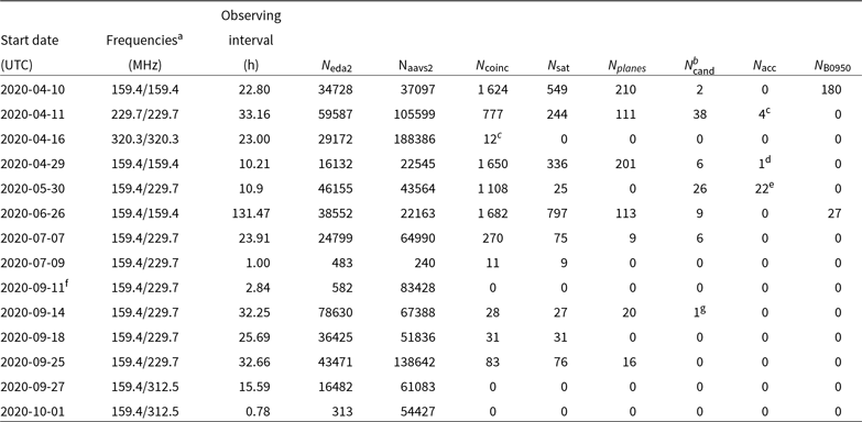
Figure 2. Examples of 2 s all-sky images from the EDA2 at 159.375 MHz collected on 2020 April 10 at 14:11:32 UTC. Left: XX image (YY image is virtually the same and not shown). The brightest sources are labelled. Right: Stokes I image, that is, average of the beam-corrected XX and YY images. The corresponding images from the AAVS2 station are very similar and not shown for brevity.
4.2.2. Flux calibration
For accurate flux calibration, the apparent flux density of the Sun was calculated by multiplying the flux density predicted by the Benz (Reference Benz2009) model by the response of the dipole beam pattern (Davidson et al. Reference Davidson2020b) in the direction of the Sun. These beam patterns were simulated in FEKO electromagnetic simulation software. It was found during the station sensitivity studies that applying a single calibration (from the transiting Sun) to long observations may result in flux density errors of the order of 20–30%. Similar variations were identified in the amplitudes of calibration solutions over many hours of calibration using low-frequency all-sky sky models, such as the sky image at 408 MHz (Haslam et al. Reference Haslam, Salter, Stoffel and Wilson1982), the so-called ‘Haslam map’, scaled down to low frequencies using a spectral index of $-2.55$
(Mozdzen et al. Reference Mozdzen, Mahesh, Monsalve, Rogers and Bowman2019) or Global Sky Model (de Oliveira-Costa et al. Reference de Oliveira-Costa, Tegmark, Gaensler, Jonas, Landecker and Reich2008). These variations of amplitudes of calibration solutions have been found to be mainly due to diurnal changes in ambient temperature. We have also tested flux density vs time (lightcurves) of two bright calibrators (Hydra A and Virgo A) and found that their flux variations were within 10% when they were above elevation
$-2.55$
(Mozdzen et al. Reference Mozdzen, Mahesh, Monsalve, Rogers and Bowman2019) or Global Sky Model (de Oliveira-Costa et al. Reference de Oliveira-Costa, Tegmark, Gaensler, Jonas, Landecker and Reich2008). These variations of amplitudes of calibration solutions have been found to be mainly due to diurnal changes in ambient temperature. We have also tested flux density vs time (lightcurves) of two bright calibrators (Hydra A and Virgo A) and found that their flux variations were within 10% when they were above elevation $40^\circ$
and 50
$40^\circ$
and 50 $^\circ$
for EDA2 and AAVS2 stations, respectively. The inaccuracy of flux density measurements at lower elevations stems mainly from the inaccuracy using a single dipole beam pattern for all station antennas, which may be significantly different from embedded elements patternsFootnote c especially for the AAVS2 station using more complex antenna and more affected by the mutual coupling effects (Davidson et al. Reference Davidson2020b).
$^\circ$
for EDA2 and AAVS2 stations, respectively. The inaccuracy of flux density measurements at lower elevations stems mainly from the inaccuracy using a single dipole beam pattern for all station antennas, which may be significantly different from embedded elements patternsFootnote c especially for the AAVS2 station using more complex antenna and more affected by the mutual coupling effects (Davidson et al. Reference Davidson2020b).
4.2.3. Other calibration methods
Although the routine calibration procedure uses Sun as a phase and flux calibrator other calibration methods have also been successfully tested. The earlier mentioned calibration using low-frequency all-sky model (so-called ‘all-sky model calibration’) leads to similar calibration solutions and is the most likely replacement for the currently used procedure. Especially, that the minimum of solar cycle 25 comes to an end, and more active Sun may soon become a very inaccurate calibrator. We note that using individual bright calibrators (so-called ‘A-team sources’), such as Centaurus A, Hercules A, Hydra A, Pictor A, 3C444, Fornax A, and Virgo A, is limited by SNR and side-lobes. These calibrators can, at best, provide SNR of the order of a few hundred (maybe $\sim$
1 000 for Centaurus A provided that good model of this source is used). However, this way of calibration has not been extensively tested yet, and is planned in the future. Especially, once the instantaneous bandwidth will be increased and/or longer calibration observations become practicable. We are expecting that the all-sky model (including A-team sources) calibration will be the most accurate method applicable over a wide range of local sidereal times (LSTs). Finally, novel calibration methods such as holography also yield very promising results (Kiefner et al. Reference Kiefner2021) and may soon become an viable alternative to standard, visibilities-based methods of station calibration.
$\sim$
1 000 for Centaurus A provided that good model of this source is used). However, this way of calibration has not been extensively tested yet, and is planned in the future. Especially, once the instantaneous bandwidth will be increased and/or longer calibration observations become practicable. We are expecting that the all-sky model (including A-team sources) calibration will be the most accurate method applicable over a wide range of local sidereal times (LSTs). Finally, novel calibration methods such as holography also yield very promising results (Kiefner et al. Reference Kiefner2021) and may soon become an viable alternative to standard, visibilities-based methods of station calibration.
4.3. All-sky imaging
The visibilities are calibrated using the set of the latest calibration solutions generated by the procedure described in Sections 4.1 and 4.2. The same set of calibration solutions is applied to all the data collected during a single acquisition as they are sufficiently stable (Section 4.2). Therefore, it is not critical to dynamically update calibration solutions during the acquisitions, but this improvement is planned in the near future.
Visibilities XX and YY from each UV FITS file are imaged with invert task using robust=-0.5 weights (no CLEAN was performed). We note that all baselines were used and no u,v cut was applied for imaging (only in calibration). The all-sky image size is calculated as $N_{\rm px} = O\pi D \nu / c$
pixels, where D is the station diameter (35 and 38 m for the EDA2 and AAVS2, respectively),
$N_{\rm px} = O\pi D \nu / c$
pixels, where D is the station diameter (35 and 38 m for the EDA2 and AAVS2, respectively), $\nu$
is the observing frequency, c is the speed of light, and the factor of O comes from required over-sampling of the beam and is typically set to
$\nu$
is the observing frequency, c is the speed of light, and the factor of O comes from required over-sampling of the beam and is typically set to $O=3$
(e.g. 180
$O=3$
(e.g. 180 $\times$
180 pixels at 159.375 MHz). The XX and YY images (examples in Figure 2) can be divided by the corresponding images of the average embedded element beam (Figure 3), but this step was only used when flux calibrated lightcurves were generated as artefacts introduced by the inaccuracies of the beam model can affect difference image-based transient searches. In the next step, XX and YY images are averaged to form Stokes I images,Footnote d which is the starting point for the presented ‘blind’ transient searches. An example Stokes I all-sky image generated by the pipeline at
$\times$
180 pixels at 159.375 MHz). The XX and YY images (examples in Figure 2) can be divided by the corresponding images of the average embedded element beam (Figure 3), but this step was only used when flux calibrated lightcurves were generated as artefacts introduced by the inaccuracies of the beam model can affect difference image-based transient searches. In the next step, XX and YY images are averaged to form Stokes I images,Footnote d which is the starting point for the presented ‘blind’ transient searches. An example Stokes I all-sky image generated by the pipeline at $159.375$
MHz is shown in the right panel of Figure 2. The all-sky Stokes I images are used in difference imaging procedure, where
$159.375$
MHz is shown in the right panel of Figure 2. The all-sky Stokes I images are used in difference imaging procedure, where $n-1$
image is subtracted from the nth image and the resulting difference images (example in Figure 4) are analysed in order to identify transient candidates, that is, find pixels exceeding a pre-defined threshold of typically 5 standard deviations of the noise (
$n-1$
image is subtracted from the nth image and the resulting difference images (example in Figure 4) are analysed in order to identify transient candidates, that is, find pixels exceeding a pre-defined threshold of typically 5 standard deviations of the noise ( $5\sigma_n$
); details will be provided in Section 5.
$5\sigma_n$
); details will be provided in Section 5.
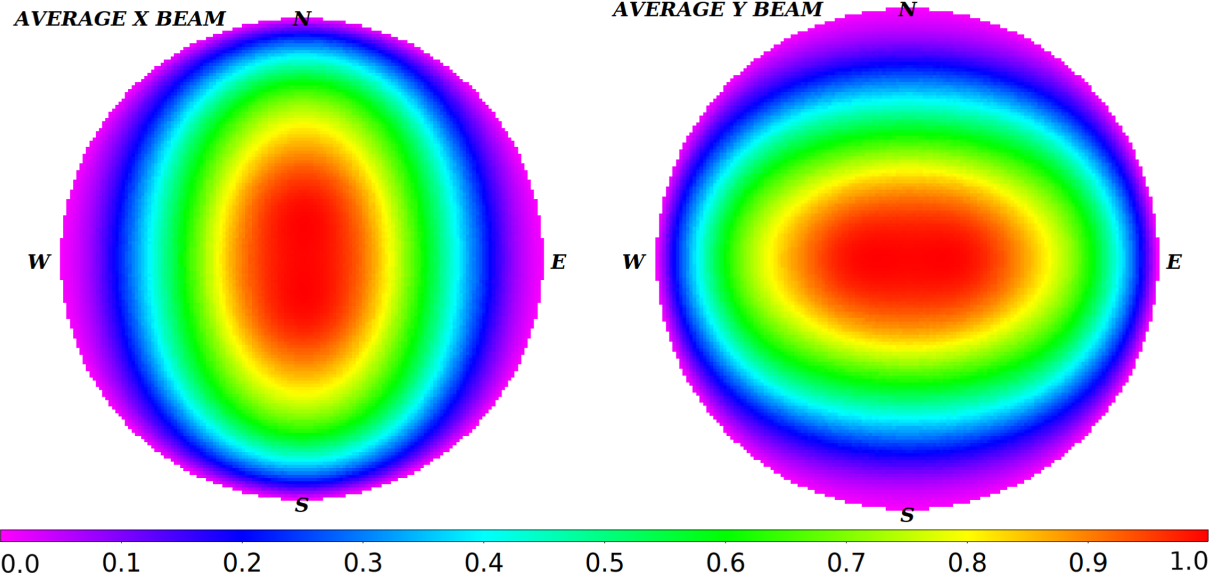
Figure 3. Examples of average beam patterns of the EDA-2 dipole in X polarisation (left) and Y polarisation (right) at 159.375 MHz. These images were used to correct the original XX and YY images for the primary beam response if correct flux scale was required to generate flux-calibrated lightcurves.
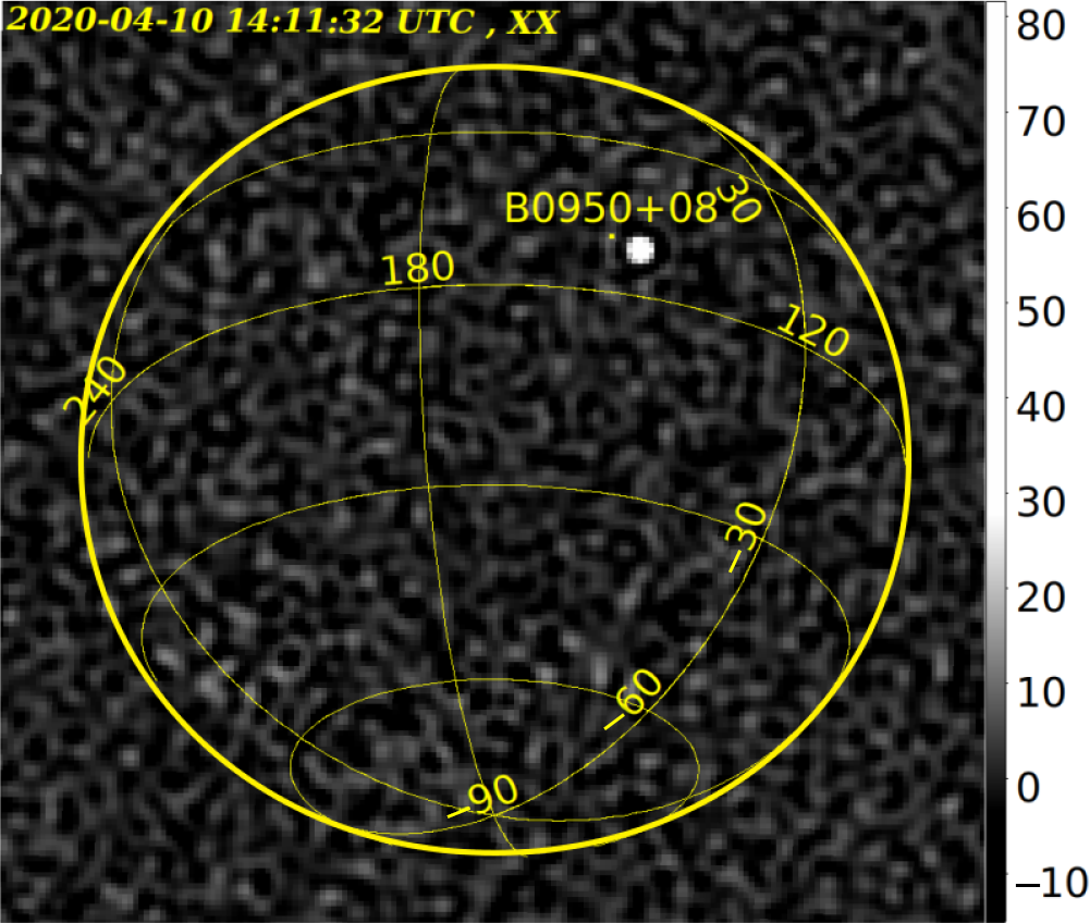
Figure 4. An example of 2 s Stokes I difference image obtained by subtracting image started on 2020 April 10 at 14:11:30 UTC from the next image started at 14:11:32 UTC. The very bright ( $\approx$
80 Jy) transient from pulsar PSR B0950+08 is clearly visible under the B0950+08 label. The thicker yellow circle represents the horizon.
$\approx$
80 Jy) transient from pulsar PSR B0950+08 is clearly visible under the B0950+08 label. The thicker yellow circle represents the horizon.
The sensitivity in terms of system equivalent flux density (SEFD) or effective area divided by system temperature (A/T) was measured from the noise in 0.14 s difference images and compared against electromagnetic simulations and SKA-Low specifications (Sokolowski et al. Reference Sokolowski, Broderick, Wayth and Davidson2021). These comparisons show that, especially at frequencies used in this paper 159.4, 229.7, and 320.1, the measured sensitivity values match the simulations very well at the time of the calibration (also single calibration was applied to long observations) and differ by at most 20–30% a few hours apart from the time of the calibration. These discrepancies are mainly caused by gain variations related to changes in ambient temperature. Furthermore, we verified that the noise in difference images has Gaussian distribution. We also calculated standard deviations of these distributions using data from the night 2020 April 10 (at 159.375 MHz) and found them to be approximately 3.6 and 4.2 Jy for the EDA2 and AAVS2 stations, respectively. We performed sensitivity simulations as described by Sokolowski et al. (Reference Sokolowski, Broderick, Wayth and Davidson2021), which predicted sensitivity averaged over 24 h (changes with LST) to be around 2 Jy in 2 s images and assuming 0.926 MHz observing bandwidth for both stations. The discrepancy of about factor of 2 has not been fully understood. However, there are several differences with respect to the analysis presented in Sokolowski et al. (Reference Sokolowski, Broderick, Wayth and Davidson2021), for example, 2 s dirty images vs 0.14 s lightly cleaned images, which can introduce some systematic effects and we leave further analysis to the future work.
Even at the highest observing frequencies $\approx$
320.3 MHz with pixel size
$\approx$
320.3 MHz with pixel size $\approx0.365^\circ$
, the sidereal sky movement of
$\approx0.365^\circ$
, the sidereal sky movement of $\approx0.00833^\circ$
over the integration time of 2 s corresponds to
$\approx0.00833^\circ$
over the integration time of 2 s corresponds to $\approx$
2.2% of the pixel size. This means that to produce a
$\approx$
2.2% of the pixel size. This means that to produce a $\gtrsim$
11 Jy false candidate due to an artefact of the image subtraction originating from the sky movement (i.e. flux ‘spill-over’ to a neighbouring pixel) a
$\gtrsim$
11 Jy false candidate due to an artefact of the image subtraction originating from the sky movement (i.e. flux ‘spill-over’ to a neighbouring pixel) a $\gtrsim$
500 Jy source is required. The maximum ionospheric offsets reported at 170–200 MHz by Loi et al. (Reference Loi2015) were of the order of 1.2 arcmin (below 1 arcmin under normal conditions), which is a similar fraction of pixel (
$\gtrsim$
500 Jy source is required. The maximum ionospheric offsets reported at 170–200 MHz by Loi et al. (Reference Loi2015) were of the order of 1.2 arcmin (below 1 arcmin under normal conditions), which is a similar fraction of pixel ( $\sim$
2.8%) and could cause similar effects if not the fact that the reported variability timescale was at the level of minutes (much longer than 2 s images). Finally, candidates in difference images may also be caused by the source noise from very bright radio-sources, as recently reported by Morgan & Ekers (Reference Morgan and Ekers2021). These effects justify the selection criteria excluding the regions around bright sources, such as the Sun, A-team sources, Galactic Plane, and Bulge, from the algorithm (as the criteria 1–4 in Section 5.2).
$\sim$
2.8%) and could cause similar effects if not the fact that the reported variability timescale was at the level of minutes (much longer than 2 s images). Finally, candidates in difference images may also be caused by the source noise from very bright radio-sources, as recently reported by Morgan & Ekers (Reference Morgan and Ekers2021). These effects justify the selection criteria excluding the regions around bright sources, such as the Sun, A-team sources, Galactic Plane, and Bulge, from the algorithm (as the criteria 1–4 in Section 5.2).
5. Real-time transient monitor
The all-sky images are produced in real-time and are immediately picked-up by the transients identification algorithm. We note, however, that at these early stages all the datasets were re-analysed off-line as the pipeline and algorithm has been undergoing very rapid development. The algorithm for transient identification has a few stages, which will be described in this section.
5.1. Source finding and transient detection
For each difference image, the standard deviation $\sigma_{n}$
of the noise in the centre of the image is calculated. In the present version, a simple source finding technique was implemented, but in the future it may be replaced by one of many existing source finding packages. All the pixels exceeding a specified threshold of 5
$\sigma_{n}$
of the noise in the centre of the image is calculated. In the present version, a simple source finding technique was implemented, but in the future it may be replaced by one of many existing source finding packages. All the pixels exceeding a specified threshold of 5 $\sigma_{n}$
are identified and nearby pixels are grouped together by selection of only the brightest pixel within a 5-pixel radius in order to avoid multiple detections of the same source.
$\sigma_{n}$
are identified and nearby pixels are grouped together by selection of only the brightest pixel within a 5-pixel radius in order to avoid multiple detections of the same source.
5.2. Filtering transient candidates
The 5 $\sigma_{n}$
transient candidates identified in the difference images from each station are initially filtered by the following station-level criteria implemented to excise false candidates due to artefacts from imperfections of difference imaging around bright radio sources:
$\sigma_{n}$
transient candidates identified in the difference images from each station are initially filtered by the following station-level criteria implemented to excise false candidates due to artefacts from imperfections of difference imaging around bright radio sources:
-
1. Galactic latitude—candidates with Galactic latitude $|b| < 10$
degrees are discarded.
$|b| < 10$
degrees are discarded. -
2. Galactic bulge—candidates with
$|b| < 15^\circ$
and Galactic longitude
$|l| < 25^\circ$
are also discarded. Both ‘Galactic coordinates’ cuts are similar to those used by Tingay et al. (Reference Tingay, Sokolowski, Wayth and Ung2020). -
3. Angular distance to Sun—candidates in angular distance from the Sun smaller than
$8^\circ$
(
$\sim$
2–4 beam sizes) are discarded. -
4. A-team sources—candidates closer than
$4^\circ$
from very bright A-team sources (Centaurus A, Hercules A, Hydra A, Pictor A, 3C444, Fornax A and Virgo A) are discarded.


The station-level criteria were designed to excise only the most common and obvious sources of false alerts and save the list of transient candidates identified by each station to text files for further processing, filtering, and post-processing analysis (including coincidence between the stations). However, some of these criteria may be relaxed in the future as the classification and filtering are improved.
In the analysis described in this paper, the source was required to be detected by both stations within a specified time window and angular distance—this requirement will be referred to as the coincidence. If the stations observed at the same frequency, the time window was set to the integration time (currently 2 s). Otherwise, the time window was determined by the maximum dispersion measure (DM) of a potential transient, which was typically set to DM = 1 000 $\text{pc cm}^{-3}$
corresponding to time window of
$\text{pc cm}^{-3}$
corresponding to time window of $\approx 84.7$
s when the stations observed at
$\approx 84.7$
s when the stations observed at $159.375$
and
$159.375$
and $229.6875$
MHz (or
$229.6875$
MHz (or $\approx 122$
s for observations at
$\approx 122$
s for observations at $159.375$
and
$159.375$
and $320.3125$
MHz). The angular distance between transient positions in the images from both stations was required to be smaller than
$320.3125$
MHz). The angular distance between transient positions in the images from both stations was required to be smaller than $3.3^\circ$
(corresponding to a station beam size at 150 MHz). The candidates accepted by the coincidence requirement were saved to a log file. The candidates detected by both stations were further filtered by the following criteria in order to flag some other sources of false alerts:
$3.3^\circ$
(corresponding to a station beam size at 150 MHz). The candidates accepted by the coincidence requirement were saved to a log file. The candidates detected by both stations were further filtered by the following criteria in order to flag some other sources of false alerts:
-
5. Elevation cut—candidates below certain elevation limit (default
$25^\circ$
) are discarded in order to avoid RFI from ground-based FM, DTV, and other transmitters in the population centres surrounding the MRO, such as Geraldton (South-West from the MRO), which is in a distance of
$\approx$
7 horizons away and can still be detected at the MRO at FM and DTV frequencies especially in favourable propagation conditions, that is, tropospheric ducting (Sokolowski, Wayth, & Ellement Reference Sokolowski, Wayth and Ellement2017; Tingay et al. Reference Tingay, Sokolowski, Wayth and Ung2020). -
6. Catalogue of satellites—each of the remaining candidates in the image is verified against the list of known satellites, which are above the horizon at the MRO at the time of the image (even up to a few hundred during a 2-s integration). In order to achieve this, every day two-line element (TLE) catalogues are downloaded from the Internet sources (e.g. www.space-track.org) and a TLE file with all the satellites (
$\sim$
16 000) is compiled for each day. Then for each image the sattest software (Sokolowski Reference Sokolowski2008) generates a list of satellites with elevation
$e > 0^\circ$
at the time when the image was collected. Next, the position of each transient candidate is verified against this list and if a satellite closer than
$4^\circ$
is found, the candidate is flagged with its NORAD ID from the TLE file. The satellites cross-matching radius
$R_{\rm sat}=4^\circ$
was selected based on a distribution of angular distances of transient candidates to the closest object from the TLE database, and as a compromise between efficiently flagging candidates due to TLE-objects and not excising all astrophysical transients because of false random cross-matches.


The number of TLE satellites ( $N_{\rm sat}$
) at elevations
$N_{\rm sat}$
) at elevations $\ge25^\circ$
at the time of each 2-s image is typically between
$\ge25^\circ$
at the time of each 2-s image is typically between $\approx$
100 and 1 000. Given that the cross-matching radius
$\approx$
100 and 1 000. Given that the cross-matching radius $R_{\rm sat}=4^\circ$
and assuming an isotropic distribution of satellites,Footnote e the probability of randomly matching a transient candidate to one of these satellites (Equation (1)) is around 50% when only about 120 TLE satellites are cross-matched. However, it reaches
$R_{\rm sat}=4^\circ$
and assuming an isotropic distribution of satellites,Footnote e the probability of randomly matching a transient candidate to one of these satellites (Equation (1)) is around 50% when only about 120 TLE satellites are cross-matched. However, it reaches $\approx$
100% for more than 240 TLE satellites and is below 1% when the number of TLE satellites at elevations
$\approx$
100% for more than 240 TLE satellites and is below 1% when the number of TLE satellites at elevations $\ge25^\circ$
is
$\ge25^\circ$
is $N_{\rm sat}\lesssim$
3 (cf. Section 6.1.1). Hence, the chances of random associations can be very high when all the TLE satellites are considered for cross-matching. This criteria is still under consideration whether only low Earth orbit (LEO) objects at a distance
$N_{\rm sat}\lesssim$
3 (cf. Section 6.1.1). Hence, the chances of random associations can be very high when all the TLE satellites are considered for cross-matching. This criteria is still under consideration whether only low Earth orbit (LEO) objects at a distance $\le$
2 000 km should be considered due to the low chances of receiving reflected signals from further objects. However, distant transmitting satellites could easily be detected. Therefore, so far we have been using the full list of satellites, not just LEO objects, but the criteria will be revised as more bandwidth and better time resolution will improve chances for automatic classification of moving objects.
$\le$
2 000 km should be considered due to the low chances of receiving reflected signals from further objects. However, distant transmitting satellites could easily be detected. Therefore, so far we have been using the full list of satellites, not just LEO objects, but the criteria will be revised as more bandwidth and better time resolution will improve chances for automatic classification of moving objects.
-
7. Catalogue of bright radio sources—each of the candidates (including those flagged as a TLE satellite) is verified against a catalogue of bright radio-sources (larger than the short list of A-team sources). If the candidate is closer than
$4^\circ$
from the source in the catalogue, it is flagged with the name of this sources and the angular distance to it is also saved to the log file.Figure 5. Distribution of all candidates detected in the 2020 April 10/11 data (red dots) and positions of all satellites above the horizon at the MRO for all the corresponding timestamps (small black dots). The black dots form clear patterns, such as geo-stationary satellites in approximately
$20^\circ$
wide belt of objects around the Equator. The observed transients detected from PSR B0950+08 form a grouping of red dots at (
$\lambda$
,
$\delta$
)
$\approx (150^\circ,10^\circ)$
and this is how these transients were first noticed among the other transient candidates. -
8. Excision of images with a bright RFI transient—if a very bright RFI transient (flux density
$\ge$
300 Jy beam–1) is identified in the images from both stations, then all the candidates from these images are rejected. This is to reject false candidates from very strong side-lobes resulting from such a bright RFI event, which can cause many false candidates across an entire image. -
9. Sun/daytime—the images collected when the Sun was above elevation of
$20^\circ$
are excluded from the analysis due to very strong side-lobes from the Sun (compare to the previous criterion). -
10. Pre-defined flight paths—candidates which are less than
$10^\circ$
from two typically used flight paths, which were fitted to moving candidates from one of the analysed nights (details in Section 6.1.3), are excised. This criterion can be extended in the future to use the actual data from the plane tracking websites in order to unambiguously excise false candidates due to RFI from planes.


The candidates not rejected by the above criteria are saved to the transient candidates log file for further inspection, while the rejected events are saved to a separate log file.
6. Preliminary results
After applying all the criteria described in Section 5.1, the transient candidates matched to TLE-catalogue satellites or A-team radio-sources are flagged and the corresponding NOARD ID or/and radio-source name and the angular distance are saved to a log file. Due to large number of known satellites (up to 1 000 when any distance is considered) above the horizon, a large fraction of the TLE-catalogue satellites cross-matches are false, which unfortunately noticeably reduces efficiency of the algorithm to detect astrophysical transients. Table 1 shows the number of candidates after subsequent criteria for 14 analysed nights ( $\approx366\,$
h in total) when data from both stations were collected simultaneously. The final list of candidates not matched to any satellite required further visual inspection. As can be seen from Table 1 in some cases, it was impossible to visually inspect all of them. However, at this stage we are not intending to do it as the number of candidates will be significantly reduced when fine channelised images, larger frequency band, and better time resolution are implemented, which will also help in excision of moving objects.
$\approx366\,$
h in total) when data from both stations were collected simultaneously. The final list of candidates not matched to any satellite required further visual inspection. As can be seen from Table 1 in some cases, it was impossible to visually inspect all of them. However, at this stage we are not intending to do it as the number of candidates will be significantly reduced when fine channelised images, larger frequency band, and better time resolution are implemented, which will also help in excision of moving objects.
Using 160 MHz images (180 $\times$
180 pixels), we verified that the number of pixels above the minimum elevation of
$\times$
180 pixels), we verified that the number of pixels above the minimum elevation of $25^\circ$
is approximately 14 261. Given the probability of exceeding the
$25^\circ$
is approximately 14 261. Given the probability of exceeding the $5\sigma_n$
threshold by the Gaussian noise is
$5\sigma_n$
threshold by the Gaussian noise is $\approx 2.86 \times 10^{-7}$
, and the requirement for the candidate to be detected by both stations at the same sky position, the expected number of false candidates in 43 200 images from 24 h of observations is
$\approx 2.86 \times 10^{-7}$
, and the requirement for the candidate to be detected by both stations at the same sky position, the expected number of false candidates in 43 200 images from 24 h of observations is $\approx$
0.7. Moreover, this very low number is before any criteria other than the coincidence and elevation cut. We confirm that we inspected all the events in the column 9 of Table 1, and none of them looked like caused by fluctuation of the noise with most of them having SNR
$\approx$
0.7. Moreover, this very low number is before any criteria other than the coincidence and elevation cut. We confirm that we inspected all the events in the column 9 of Table 1, and none of them looked like caused by fluctuation of the noise with most of them having SNR $\gtrsim10$
.
$\gtrsim10$
.
6.1. Radio frequency-interference
6.1.1. Satellites
The positions of identified transient candidates were compared to positions calculated for objects in the TLE database (typically about 16 600 objects) using the SATTEST program. Figure 5 shows distribution of all transient candidates identified in the 2020 April 10/11 data overplotted with calculated positions of all satellites above the horizon at the MRO at the times of the identified transients. The patterns in expected orbital positions of TLE satellites are clearly visible (e.g. geo-stationary satellites forming an approximately $20^\circ$
wide strip of objects around the Equator). It was also verified that over the 24 h interval starting at around 21:30 AWST on 2020 April 10 the number of satellites at elevations
$20^\circ$
wide strip of objects around the Equator). It was also verified that over the 24 h interval starting at around 21:30 AWST on 2020 April 10 the number of satellites at elevations $\ge25^\circ$
in an arbitrary distance from the Earth was between 860 and 1 010, while number of only LEO satellites (height
$\ge25^\circ$
in an arbitrary distance from the Earth was between 860 and 1 010, while number of only LEO satellites (height $\le$
2 000 km) was between 85 and 170. Given the number of TLE-catalogue satellites
$\le$
2 000 km) was between 85 and 170. Given the number of TLE-catalogue satellites ${N}_{\rm sat}$
above elevation
${N}_{\rm sat}$
above elevation ${e}_{\min}$
at a particular moment, the excision radius
${e}_{\min}$
at a particular moment, the excision radius ${R}_{\rm coinc}$
and minimum considered elevation
${R}_{\rm coinc}$
and minimum considered elevation ${e}_{\min}$
the probability, p, of randomly matching a TLE-catalogue satellite to a transient candidate can be calculated as:
${e}_{\min}$
the probability, p, of randomly matching a TLE-catalogue satellite to a transient candidate can be calculated as:
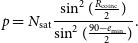 \begin{equation}p = N_{\rm sat} \frac{\sin^2(\frac{R_{\rm coinc}}{2})}{\sin^2(\frac{90 - e_{\min}}{2})}.\end{equation}
Assuming uniform distribution of satellites, which as Figure 5 shows, is not an ideal approximation, and equation 1 results in the probability (p) of falsely matching a transient candidate to a TLE satellite greater than one (between 3.6 and 4.3) for satellites at an arbitrary distance from the Earth, and 0.36–0.72 for LEO satellites (mean 0.54). These probabilities are in an order-of-magnitude agreement with our analysis. When the transient candidates were cross-matched against TLE satellites in an arbitrary distance from the Earth, then $\approx$
92% of transient candidates were matched to a TLE satellite. The disagreement (
$\approx$
92% of transient candidates were matched to a TLE satellite. The disagreement ( $>$
100% probability expected vs 92% probability observed) is most likely due to the fact that the satellite positions are not isotropically distributed and are clustered around certain orbits (e.g. geo-stationary) and because of this clustering the probability of matching transients at any sky coordinates is lower than predicted for an isotropic distribution of satellites. Therefore, many of the real astrophysical transients from PSR B0950+08 were not excised by this criterion. On the other hand, when only LEO satellites were cross-matched, the percentage of transient candidates matched to LEO satellites was approximately 55%, which is close to the predicted value of 54%, indicating that for these objects the isotropic distribution assumption is indeed valid. The full description of these probabilities requires more simulation work and is beyond the scope of this paper, but will be performed if required by the future analysis. Clearly, excision of satellites using a catalogue of orbital elements is not an optimal approach, but it may not be required once the increased bandwidth and better frequency and time resolutions become available.
$>$
100% probability expected vs 92% probability observed) is most likely due to the fact that the satellite positions are not isotropically distributed and are clustered around certain orbits (e.g. geo-stationary) and because of this clustering the probability of matching transients at any sky coordinates is lower than predicted for an isotropic distribution of satellites. Therefore, many of the real astrophysical transients from PSR B0950+08 were not excised by this criterion. On the other hand, when only LEO satellites were cross-matched, the percentage of transient candidates matched to LEO satellites was approximately 55%, which is close to the predicted value of 54%, indicating that for these objects the isotropic distribution assumption is indeed valid. The full description of these probabilities requires more simulation work and is beyond the scope of this paper, but will be performed if required by the future analysis. Clearly, excision of satellites using a catalogue of orbital elements is not an optimal approach, but it may not be required once the increased bandwidth and better frequency and time resolutions become available.
Finally, it can be calculated (Equation (1)) that the probability of matching a specific satellite (with a given NORAD ID) to a transient candidate is very low $\sim$
0.3% and therefore the probability of randomly matching the same satellite more than 5 times is
$\sim$
0.3% and therefore the probability of randomly matching the same satellite more than 5 times is $\lesssim10^{-13}$
. Hence, it can be assumed that multiple matches to the same satellite are genuine identifications of this satellite. Figure 6 shows the number of satellite observations per unique NORAD ID for the data from night 2020 April 10/11. The distribution peaks at a very low number of matches and falls-off rapidly indicating that the majority of cross-matches are random false identifications. However, the peak at 123 matches is due to BGUSAT (NORAD ID 41999), which has been confirmed to be a genuine detection. BGUSAT is a nanosatellite which has been regularly detected in the EDA2 and AAVS2 data at many observing frequencies and it is most likely transmitting out of its nominal band (Tingay et al. Reference Tingay, Sokolowski, Wayth and Ung2020). Example detections of BGUSAT at 159.375 MHz are shown in Figure 7. Other NORAD IDs with more than 10 matches are summarised in Table 2. This table shows that, while there are satellites (like BGUSAT) likely transmitting at wide range of frequencies 159.4 and 229.7 MHz and in FM band (Tingay et al. Reference Tingay, Sokolowski, Wayth and Ung2020), in general a completely different group of satellites have been detected at frequencies above 229.7 MHz (mostly Russian COSMOS class satellites). We also note that no satellites were identified when both stations observed at about 320.3 MHz (2020 April 16/17 data), which seems to be a very clean band to look for transients. The objects in Table 2 are different from those detected with the MWA in 72.335–103.015 MHz band (partially overlapping with the FM band) by the earlier studies (Prabu et al. Reference Prabu, Hancock, Zhang and Tingay2020b, 2020a; Zhang et al. Reference Zhang2018).
$\lesssim10^{-13}$
. Hence, it can be assumed that multiple matches to the same satellite are genuine identifications of this satellite. Figure 6 shows the number of satellite observations per unique NORAD ID for the data from night 2020 April 10/11. The distribution peaks at a very low number of matches and falls-off rapidly indicating that the majority of cross-matches are random false identifications. However, the peak at 123 matches is due to BGUSAT (NORAD ID 41999), which has been confirmed to be a genuine detection. BGUSAT is a nanosatellite which has been regularly detected in the EDA2 and AAVS2 data at many observing frequencies and it is most likely transmitting out of its nominal band (Tingay et al. Reference Tingay, Sokolowski, Wayth and Ung2020). Example detections of BGUSAT at 159.375 MHz are shown in Figure 7. Other NORAD IDs with more than 10 matches are summarised in Table 2. This table shows that, while there are satellites (like BGUSAT) likely transmitting at wide range of frequencies 159.4 and 229.7 MHz and in FM band (Tingay et al. Reference Tingay, Sokolowski, Wayth and Ung2020), in general a completely different group of satellites have been detected at frequencies above 229.7 MHz (mostly Russian COSMOS class satellites). We also note that no satellites were identified when both stations observed at about 320.3 MHz (2020 April 16/17 data), which seems to be a very clean band to look for transients. The objects in Table 2 are different from those detected with the MWA in 72.335–103.015 MHz band (partially overlapping with the FM band) by the earlier studies (Prabu et al. Reference Prabu, Hancock, Zhang and Tingay2020b, 2020a; Zhang et al. Reference Zhang2018).
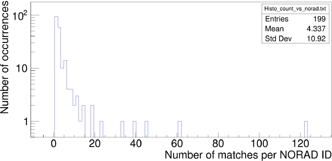
Figure 6. Number of transient candidates matches per NORAD ID for the data from night 2020 April 10/11. The peak at 123 corresponds to BGUSAT (NORAD ID 41999).
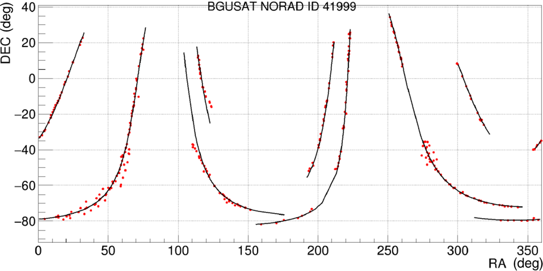
Figure 7. Example detections of BGUSAT (NORAD ID 41999) in AAVS2 difference images at 159.375 MHz (red points) and predicted paths (black curves). Several few minute-long passages were observed between 2020 June 26 21:15:42 and 2020 July 2 08:44:05 AWST. In order to create this image, the transient searching algorithm was executed without any restrictions on the Sun elevation.
Table 2. A list of TLE objects most commonly detected with the system and having at least 10 matches (except a few special cases). In order to create this table, the filtering criteria were relaxed to allow daytime and minimum elevation of transient candidate of $15^\circ$
(nominally transients are searched in night-time data only and at elevations
$15^\circ$
(nominally transients are searched in night-time data only and at elevations $\ge25^\circ$
). Additional information in columns 5, 6, and 7 was obtained from Tingay et al. (Reference Tingay, Sokolowski, Wayth and Ung2020), the web pages https://www.n2yo.com/satellite/?s=NORADID and http://www.zarya.info/Frequencies/FrequenciesAll.php, where NORADID has to be replaced by a value from the first column of this table. For the rocket bodies, space debris, and other inactive elements, the 5-th column contains N/A value. The values of radar cross-section (RCS) in column 7 are poorly known and represent the best estimates we could find. At these frequencies, the most likely sources of reflected signal are ground-based transmitters. However, except the frequency 229.6875 MHz, they cannot be DTV or FM transmitters located in Australia (see discussion in Section 6.1.2)
$\ge25^\circ$
). Additional information in columns 5, 6, and 7 was obtained from Tingay et al. (Reference Tingay, Sokolowski, Wayth and Ung2020), the web pages https://www.n2yo.com/satellite/?s=NORADID and http://www.zarya.info/Frequencies/FrequenciesAll.php, where NORADID has to be replaced by a value from the first column of this table. For the rocket bodies, space debris, and other inactive elements, the 5-th column contains N/A value. The values of radar cross-section (RCS) in column 7 are poorly known and represent the best estimates we could find. At these frequencies, the most likely sources of reflected signal are ground-based transmitters. However, except the frequency 229.6875 MHz, they cannot be DTV or FM transmitters located in Australia (see discussion in Section 6.1.2)
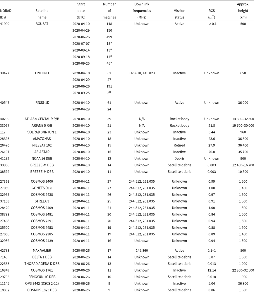
aIt was observed that BGUSAT was much brighter ( $\sim$
30–250 times) at 159.375 MHz (
$\sim$
30–250 times) at 159.375 MHz ( $\sim$
900 Jy beam–1) than at 230 MHz (
$\sim$
900 Jy beam–1) than at 230 MHz ( $\sim$
30 Jy beam–1).
$\sim$
30 Jy beam–1).
bOnly 3 detections, but shown here to exemplify another detection much brighter (nearly 230 times) at 159.375 MHz ( $\sim$
7700 Jy beam–1) than at 230 MHz (
$\sim$
7700 Jy beam–1) than at 230 MHz ( $\sim$
34 Jy beam–1).
$\sim$
34 Jy beam–1).
6.1.2. Origin of the signals
Given large uncertainties in radar cross-sections (RCS) for the majority of the detected objects, the full analysis of the detected signals being due reflections or transmissions is beyond the scope of this paper. A possible source of signals for these reflections at the analysed frequencies are ground-based transmitters in Western Australia or possibly beyond (subject to power constraints). Nevertheless, out of all the frequency channels used in the presented analysis, only the frequency channel 229.6875 MHz is within the frequency band of DTV transmitters in Australia, which extends up to 230 MHz (see, e.g., Figure 2 in Sokolowski, Wayth, & Lewis Reference Sokolowski, Wayth and Lewis2015). Specifically, there are 50 kW DTV transmitters in Perth covering frequency band 170–230 MHz. None of the other frequency channels used in this analysis are within the frequency bands allocated for broadcasting (see Australian Communications and Median AuthorityFootnote f). Hence, the potential reflections could not be due to DTV or FM transmitters. The signal sources for the potential reflections at frequencies other than 229.6875 MHz could be located outside Australia, but we did not explore the list of frequencies and transmitters in the nearest countries. Nevertheless, we provide a simple estimate of the expected flux densities. Assuming isotropic gain of ground-based DTV transmitters of power ${P}_{\text{tr}}^{\text{kW}}$
(in kW) radiating uniformly over the
${P}_{\text{tr}}^{\text{kW}}$
(in kW) radiating uniformly over the $\text{BW}_{\text{MHz}}^{\text{tr}}$
band (7 MHz for DTV) as source of the reflected signal, equal distance
$\text{BW}_{\text{MHz}}^{\text{tr}}$
band (7 MHz for DTV) as source of the reflected signal, equal distance ${r}_{\text{km}}$
(in km) from transmitter to receiver in a bi-static radar configuration, and using a textbook radar equation, the following equation can be derived to estimate expected flux density due to reflections:
${r}_{\text{km}}$
(in km) from transmitter to receiver in a bi-static radar configuration, and using a textbook radar equation, the following equation can be derived to estimate expected flux density due to reflections:
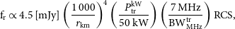 \begin{equation}\text{f}_{\text{r}} \propto \text{4.5\,[mJy]} \left( \frac{\text{1\,000}}{{r}_{\text{km}}} \right)^4 \left( \frac{{P}_{\text{tr}}^{\text{kW}}}{\text{50 kW}} \right) \left( \frac{\text{7\,MHz}}{\text{BW}_{\text{MHz}}^{\text{tr}}} \right) \text{RCS},\end{equation}
where RCS is in m $^2$
. Given that flux densities observed for the objects in Table 2 are in the range from tens to a few thousands Jy, it is nearly impossible that they are caused by off-the-satellites reflections of signals emitted by DTV or other ground-based transmitters in Western Australia or further. Using BGUSAT at the height about 500 km as an example, the expected flux density from a 50 kW transmitter in Perth would be below 7.2 mJy, while the observed flux densities of BGUSAT were in the range 10–3 500 Jy. The observed flux densities are much more consistent with line-of-sight propagation from a low power transmitter (
$^2$
. Given that flux densities observed for the objects in Table 2 are in the range from tens to a few thousands Jy, it is nearly impossible that they are caused by off-the-satellites reflections of signals emitted by DTV or other ground-based transmitters in Western Australia or further. Using BGUSAT at the height about 500 km as an example, the expected flux density from a 50 kW transmitter in Perth would be below 7.2 mJy, while the observed flux densities of BGUSAT were in the range 10–3 500 Jy. The observed flux densities are much more consistent with line-of-sight propagation from a low power transmitter ( $\le$
1 W) with a small fraction of out-of-band ‘spill-over’ over a wide frequency band.
$\le$
1 W) with a small fraction of out-of-band ‘spill-over’ over a wide frequency band.
6.1.3. Aircraft
Bright transient candidates were identified to be mostly due to airplanes passing in the close vicinity of the MRO. Two main routes were identified and a parabola in elevation vs azimuth was fitted to a set candidates from 2020 April 10/11 brighter than 300 Jy beam–1 (black crosses in Figure 8). The relatively low threshold of 300 Jy beam–1 was chosen to fit the curves to a sufficiently large number of points. These two parabolas were later used to excise transient candidates if they were closer than three times beam size ( $\approx10^\circ$
). This is not an ideal criterion because the routes of planes may vary between days. Therefore, in the future we will try to automatically fit tracks to the moving objects, use time and frequency resolution (once coarse channel data are channelised and images in fine channels are formed), and if still required, use aircraft tracking services to obtain coordinates of aircraft in the vicinity of the MRO. These signals may be caused by reflections off nearby (within tens of km) airplanes (with RCS
$\approx10^\circ$
). This is not an ideal criterion because the routes of planes may vary between days. Therefore, in the future we will try to automatically fit tracks to the moving objects, use time and frequency resolution (once coarse channel data are channelised and images in fine channels are formed), and if still required, use aircraft tracking services to obtain coordinates of aircraft in the vicinity of the MRO. These signals may be caused by reflections off nearby (within tens of km) airplanes (with RCS $\gtrsim$
2m
$\gtrsim$
2m $^2$
). It can be shown, using Equation (2), that reflections of signals emitted over a narrow band (
$^2$
). It can be shown, using Equation (2), that reflections of signals emitted over a narrow band ( $\sim$
10 kHz) by even low power (
$\sim$
10 kHz) by even low power ( $\le$
1 W) ground-based transmitters can cause high flux density candidates (of the order of thousands of Jy).
$\le$
1 W) ground-based transmitters can cause high flux density candidates (of the order of thousands of Jy).
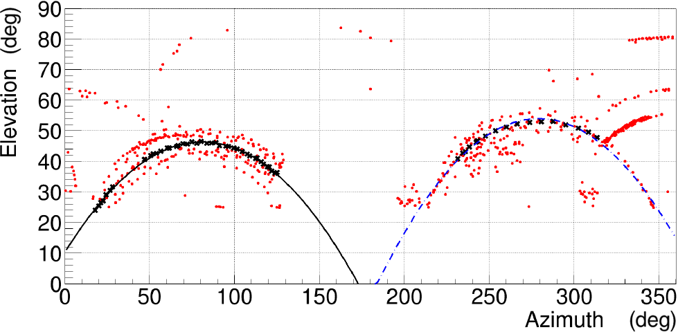
Figure 8. Transient candidates from 2020 April 10/11 data overplotted with second-order polynomials fitted to two paths. These parabolas were later used in excising RFI from aircraft moving along these routes.
The distance between the two stations is approximately 165 m. Therefore, the very near-Earth objects (like planes) can be observed in the images from two stations at slightly different positions with respect to stars due to parallax effect, which could be used to excise these kind of objects. We assume that the minimum measurable angular distance is $\sim\frac{1}{5}$
of the synthesised beam (
$\sim\frac{1}{5}$
of the synthesised beam ( $\approx2.3^\circ$
and
$\approx2.3^\circ$
and $\approx1.15^\circ$
at 160 and 320 MHz, respectively). Therefore, the maximum altitude to which parallax can be observed is 21 and 41 km at 160 and 320 MHz, respectively (assuming a plane flying overhead). Since, our spatial coincidence radius (
$\approx1.15^\circ$
at 160 and 320 MHz, respectively). Therefore, the maximum altitude to which parallax can be observed is 21 and 41 km at 160 and 320 MHz, respectively (assuming a plane flying overhead). Since, our spatial coincidence radius ( $3.3^\circ$
) is larger than the parallax angles at these frequencies we did not take advantage of this effect in the presented analysis. However, in the future if the positions of objects are indeed determined with the accuracy of at least
$3.3^\circ$
) is larger than the parallax angles at these frequencies we did not take advantage of this effect in the presented analysis. However, in the future if the positions of objects are indeed determined with the accuracy of at least $\sim\frac{1}{5}$
of the synthesised beam, it will be possible to use the parallax to excise objects closer than
$\sim\frac{1}{5}$
of the synthesised beam, it will be possible to use the parallax to excise objects closer than $\sim$
41 km. However, the efficacy of this criterion may be limited to aircraft flying over-head as for the objects closer to the horizon (distance to horizon is
$\sim$
41 km. However, the efficacy of this criterion may be limited to aircraft flying over-head as for the objects closer to the horizon (distance to horizon is $\approx700\,$
km for objects at altitude 40 km) the parallax angles will be smaller than the achievable angular resolution.
$\approx700\,$
km for objects at altitude 40 km) the parallax angles will be smaller than the achievable angular resolution.
6.2. PSR B0950+08
The candidate events identified by the ‘blind’ search algorithm described in Section 5.1 and passing all the criteria were visually examined, and a summary is given in Table 1. A majority of these candidates were seen as single image transients, which we could not assign to any of the satellites in the database, nor match to any pre-defined flight paths (Section 6.1.3). A large grouping of these candidates near the position of PSR B0950+08 was identified in the 2020 April 10/11 data (Figure 5 and Table 1), which we interpret as bright pulses from the pulsar and discuss in this section. We however note that our 2 s integration time means averaging over approximately 8 rotation periods ( $P\approx 0.253$
s), and hence these events are not individual bright pulses, although they necessarily imply that there were multiple bright individual pulses in the corresponding integration. We hence refer to these ‘events’ as bright pulses. This also means that some of the individual pulses in a given integration are likely much brighter than that appear to be in our analysis.
$P\approx 0.253$
s), and hence these events are not individual bright pulses, although they necessarily imply that there were multiple bright individual pulses in the corresponding integration. We hence refer to these ‘events’ as bright pulses. This also means that some of the individual pulses in a given integration are likely much brighter than that appear to be in our analysis.
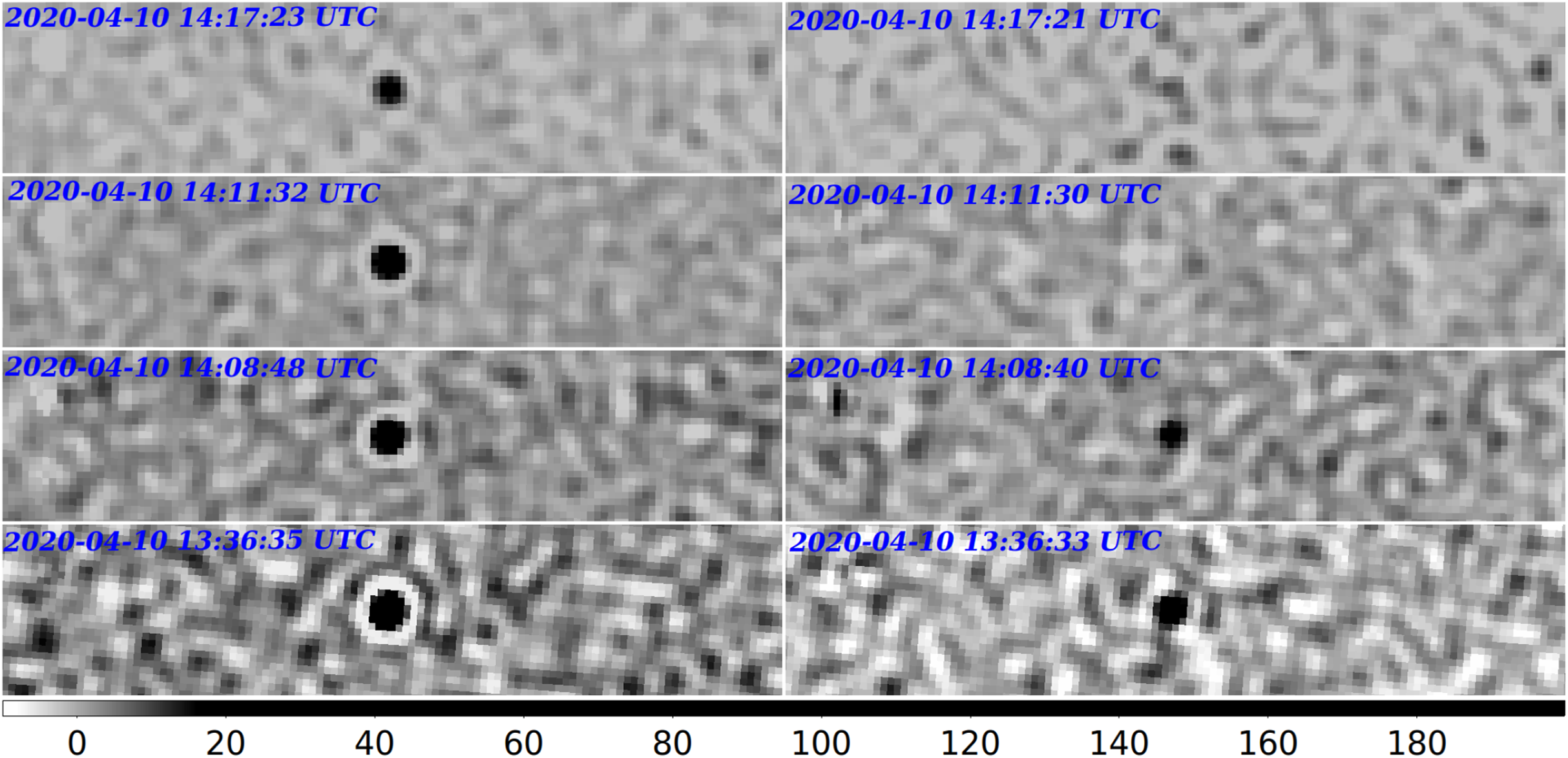
Figure 9. Stokes I difference images of the four brightest pulses from PSR B0950+08 2 s (left column) and the preceding 2 s images (right column). The images were obtained from Stokes I images after subtracting a running median of 30 images from the original images because it was very difficult to see the transients in the original images.
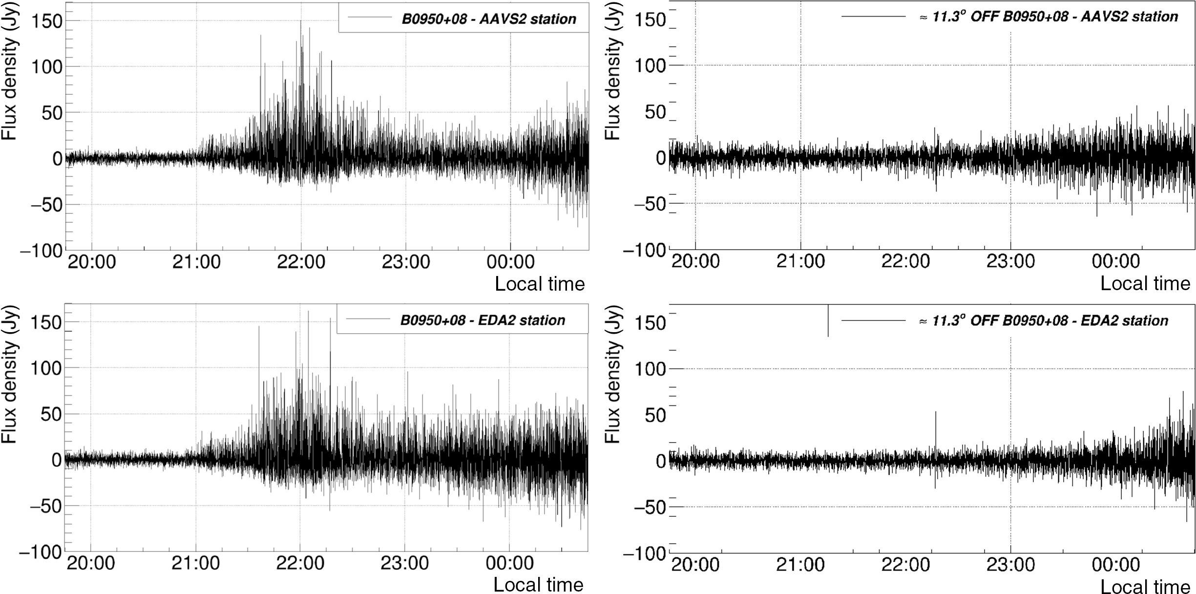
Figure 10. Left: the lightcurve of PSR B0950+08 based on the data from the EDA2 (lower image) and AAVS2 (top image) collected at 159.375 MHz between 2020 April 10 11:30 UTC and 2020 April 11 11:30 UTC (only data when pulsar was above elevation $\approx30^\circ$
are shown). It was obtained from the flux density at the position of pulsar and after subtraction of the running median of 30 points around this timestamp (excluding the value at the current timestamp). The flux densities are consistent between both stations and the peak flux density reached maximum of
$\approx30^\circ$
are shown). It was obtained from the flux density at the position of pulsar and after subtraction of the running median of 30 points around this timestamp (excluding the value at the current timestamp). The flux densities are consistent between both stations and the peak flux density reached maximum of $\approx$
150 Jy beam–1 (i.e. fluence
$\approx$
150 Jy beam–1 (i.e. fluence $\approx$
300 kJy ms) at 2020 April 10 at 14:04:47 UTC. The standard deviation of the noise in the pulsar ‘quiet time’ (before 13 UTC) was approximately 3.8 Jy beam–1 and 3.6 Jy beam–1 for the EDA2 and AAVS2 stations, respectively. Right: a reference lightcurve at a position slightly away (
$\approx$
300 kJy ms) at 2020 April 10 at 14:04:47 UTC. The standard deviation of the noise in the pulsar ‘quiet time’ (before 13 UTC) was approximately 3.8 Jy beam–1 and 3.6 Jy beam–1 for the EDA2 and AAVS2 stations, respectively. Right: a reference lightcurve at a position slightly away ( $\approx11.3^\circ$
) from the pulsar with the EDA2 (lower image) and AAVS2 (top image). The standard deviation of the noise is approximately 4.9 Jy beam–1 and 7.2 Jy beam–1 for the EDA2 and AAVS2, respectively (for the data before 13:00 UTC). In both lightcurves, the noise increased at later times after the Galactic Centre rose above the horizon at 13:30 UTC and especially after it reached
$\approx11.3^\circ$
) from the pulsar with the EDA2 (lower image) and AAVS2 (top image). The standard deviation of the noise is approximately 4.9 Jy beam–1 and 7.2 Jy beam–1 for the EDA2 and AAVS2, respectively (for the data before 13:00 UTC). In both lightcurves, the noise increased at later times after the Galactic Centre rose above the horizon at 13:30 UTC and especially after it reached $30^\circ$
elevation at around 16:00 UTC.
$30^\circ$
elevation at around 16:00 UTC.
Table 3. Number of 5 and 10 $\sigma_n$
pulses (
$\sigma_n$
pulses ( ${N}_{\text{B0950}}^{5\sigma}$
and
${N}_{\text{B0950}}^{5\sigma}$
and ${N}_{\text{B0950}}^{10\sigma}$
columns, respectively) from PSR B0950+08 observed in each dataset. These values were calculated using the lighcurves generated from the difference images with additional cleaning criteria (Section 6.2.1) and used as an indicator of the pulsars’s activity, while the lightcurve with the more exact background subtraction (using the running median) was generated only when the pulsar was found to be active
${N}_{\text{B0950}}^{10\sigma}$
columns, respectively) from PSR B0950+08 observed in each dataset. These values were calculated using the lighcurves generated from the difference images with additional cleaning criteria (Section 6.2.1) and used as an indicator of the pulsars’s activity, while the lightcurve with the more exact background subtraction (using the running median) was generated only when the pulsar was found to be active
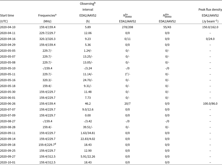
aFrequencies are approximated to a first decimal digit with the exact frequencies 159.375, 229.6875, 312.5 and 320.3125 MHz.
bWhen PSR B0950+08 was above elevation $20^\circ$
cThis pulse 27.3 Jy was only observed in images from the X polarisation (and not in Y polarisation). Thus, it was excised as RFI.
dStrong RFI was observed during some part of the night at the AAVS2 frequency of 229.7 MHz, which was possibly caused by a tropospheric ducting event.
Example difference images from the night 2020 April 10/11 with a running median of 30 images subtracted are shown in Figure 9. The detection of extreme activity from the pulsar PSR B0950+08, with maximum Stokes I flux density reaching 150 Jy beam–1, was one of the most intriguing detections so far. The lightcurves of the pulsar during the night 2020 April 10/11 are shown in the left panel of Figure 10. The EDA2 and AAVS2 station beams at 160 MHz are of order $3^\circ$
. Therefore, a single pixel may contain multiple sources, and in order to show variations at the position of PSR B0950+08 a running median of 30 points before and after each timestamp (excluding the timestamp itself) was subtracted from the flux density values at any given timestamp. Moreover, a reference lightcurve of a neighbouring off-the-pulsar position (
$3^\circ$
. Therefore, a single pixel may contain multiple sources, and in order to show variations at the position of PSR B0950+08 a running median of 30 points before and after each timestamp (excluding the timestamp itself) was subtracted from the flux density values at any given timestamp. Moreover, a reference lightcurve of a neighbouring off-the-pulsar position ( $\approx11.3^\circ$
away from the pulsar) is also shown in the right panel of Figure 10 and except for one RFI spike (at around 22:15 AWST) it does not show any significant flux density variations. These two lightcurves were constructed from the final Stokes I images after subtraction of the running median. It was verified that, unlike some of the spikes spatially coinciding with the pulsar position caused by RFI, the genuine bright pulses from PSR B0950+08 were visible in images in both X and Y polarisations.
$\approx11.3^\circ$
away from the pulsar) is also shown in the right panel of Figure 10 and except for one RFI spike (at around 22:15 AWST) it does not show any significant flux density variations. These two lightcurves were constructed from the final Stokes I images after subtraction of the running median. It was verified that, unlike some of the spikes spatially coinciding with the pulsar position caused by RFI, the genuine bright pulses from PSR B0950+08 were visible in images in both X and Y polarisations.
The 2020 April 10/11 data from both stations observing at $\approx$
159.4 MHz show very unusual, extremely bright pulses from the PSR B0950+08 with 278 and 208 pulses from the EDA2 and AAVS2 stations, respectively. The brightest observed transients (
$\approx$
159.4 MHz show very unusual, extremely bright pulses from the PSR B0950+08 with 278 and 208 pulses from the EDA2 and AAVS2 stations, respectively. The brightest observed transients ( $\sim$
155 Jy) exceed the mean flux density
$\sim$
155 Jy) exceed the mean flux density $\approx$
2.37 Jy at 150 MHz (Lorimer et al. Reference Lorimer, Yates, Lyne and Gould1995) by a factor up to even
$\approx$
2.37 Jy at 150 MHz (Lorimer et al. Reference Lorimer, Yates, Lyne and Gould1995) by a factor up to even $\sim$
65. Interestingly, they were initially discovered in the ‘blind’ search performed on the 2020 April 10/11 dataset. A very similar ‘blind’ detection of extremely bright pulses from PSR B0950+08 was also obtained by the AARTFAAC experiment (Kuiack et al. Reference Kuiack, Wijers, Rowlinson, Shulevski, Huizinga, Molenaar and Prasad2020c), where the authors concluded that these are micro-second giant pulses (GPs) similar to those observed in the Crab pulsar (PSR B0531+21 or J0534+2200; Staelin & Reifenstein 1968).
$\sim$
65. Interestingly, they were initially discovered in the ‘blind’ search performed on the 2020 April 10/11 dataset. A very similar ‘blind’ detection of extremely bright pulses from PSR B0950+08 was also obtained by the AARTFAAC experiment (Kuiack et al. Reference Kuiack, Wijers, Rowlinson, Shulevski, Huizinga, Molenaar and Prasad2020c), where the authors concluded that these are micro-second giant pulses (GPs) similar to those observed in the Crab pulsar (PSR B0531+21 or J0534+2200; Staelin & Reifenstein 1968).
6.2.1. Verification of activity during multiple nights
In an effort to verify how frequent are the episodes of such extreme activity, we have analysed 24 nights ( $\approx$
358.5 h) spread over an interval of nearly 6 months. For a quick assessment of whether the pulsar was active, we used difference images and for each station generated a lightcurve using these images with flux density measured at the position of the pulsar over the full interval of each observation. This procedure was prone to occasional bright RFI transients due to reflections or transmissions from satellites or planes. We have also found that relatively bright false detections can be generated by side-lobes from very bright RFI with flux densities of the order of thousands Jy beam–1. Therefore, in order to calculate the number of 5 and 10
$\approx$
358.5 h) spread over an interval of nearly 6 months. For a quick assessment of whether the pulsar was active, we used difference images and for each station generated a lightcurve using these images with flux density measured at the position of the pulsar over the full interval of each observation. This procedure was prone to occasional bright RFI transients due to reflections or transmissions from satellites or planes. We have also found that relatively bright false detections can be generated by side-lobes from very bright RFI with flux densities of the order of thousands Jy beam–1. Therefore, in order to calculate the number of 5 and 10 $\sigma_n$
pulses in the lightcurves, we filtered them by requiring that: (i) there is no spike of the same significance in the lightcurve generated from the pixel values at the off-pulsar position
$\sigma_n$
pulses in the lightcurves, we filtered them by requiring that: (i) there is no spike of the same significance in the lightcurve generated from the pixel values at the off-pulsar position $\approx11.3^\circ$
away from PSR B0950+08; (ii) there is no very bright RFI (exceeding the threshold of 2 500 Jy beam–1) identified in the images from a corresponding station within time interval
$\approx11.3^\circ$
away from PSR B0950+08; (ii) there is no very bright RFI (exceeding the threshold of 2 500 Jy beam–1) identified in the images from a corresponding station within time interval $\pm$
integration time (2 s) around the PSR B0950+08 pulse time. The same procedure was uniformly applied to all analysed data to calculate the number of bright PSR B0950+08 pulses in the data from both stations and the results are summarised in Table 3.
$\pm$
integration time (2 s) around the PSR B0950+08 pulse time. The same procedure was uniformly applied to all analysed data to calculate the number of bright PSR B0950+08 pulses in the data from both stations and the results are summarised in Table 3.
Besides the 2020 April 10/11, bright pulses were found only in two other datasets. Much fewer (20 by EDA2 and 7 by AAVS2) bright pulses ( $\sim$
100 Jy beam–1) from PSR B0950+08 were observed in the data from 2020 June 26/28 when both stations also observed at
$\sim$
100 Jy beam–1) from PSR B0950+08 were observed in the data from 2020 June 26/28 when both stations also observed at $\approx$
159.4 MHz. Finally, bright pulses from PSR B0950+08 were also detected at another frequency in a single dataset (2020 April 16) when both stations observed at 320.3 MHz and 11 weak pulses (
$\approx$
159.4 MHz. Finally, bright pulses from PSR B0950+08 were also detected at another frequency in a single dataset (2020 April 16) when both stations observed at 320.3 MHz and 11 weak pulses ( $\lesssim$
24 Jy beam–1) were detected only by the AAVS2 station (Table 3). No sufficiently bright pulses from PSR B0950+08 were detected in other datasets. Hence, based on the total time of
$\lesssim$
24 Jy beam–1) were detected only by the AAVS2 station (Table 3). No sufficiently bright pulses from PSR B0950+08 were detected in other datasets. Hence, based on the total time of $\approx$
358.5 h on PSR B0950+08 spread over nearly 6 months, it is clear that the extreme activity observed in the data 2020 April 10/11 is very rare and appears to be less common than refractive or diffractive scintillation events.
$\approx$
358.5 h on PSR B0950+08 spread over nearly 6 months, it is clear that the extreme activity observed in the data 2020 April 10/11 is very rare and appears to be less common than refractive or diffractive scintillation events.
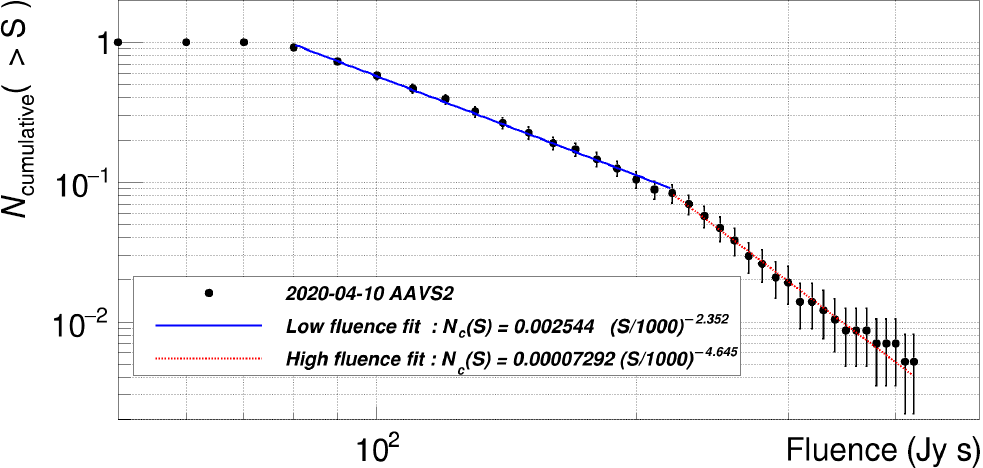
Figure 11. The cumulative distribution of bright pulses from PSR B0950+08 as observed by the AAVS2 station in the 2020 April 10/11 data. The pulse brightness was obtained by subtracting the running median. The distribution can be described with a shallower power law (fitted index $\alpha_{\rm low} \approx -2.4$
) below
$\alpha_{\rm low} \approx -2.4$
) below $F_b$
=220 Jy s (corresponding to
$F_b$
=220 Jy s (corresponding to $\approx$
360 average pulse fluences) and steeper power law above
$\approx$
360 average pulse fluences) and steeper power law above $F_b$
with
$F_b$
with $\alpha_{\rm high} \approx -4.6$
.
$\alpha_{\rm high} \approx -4.6$
.
6.2.2. Pulse fluence distribution
Figure 11 shows the fluence distribution of the pulses detected with the AAVS2 station obtained after subtracting a running median. The corresponding distribution from the EDA2 station is nearly the same and was not shown for brevity. It can be clearly seen that the slope of the distribution changes at approximate fluence $F_b$
=220 Jy s, with the fitted power law index below this
$F_b$
=220 Jy s, with the fitted power law index below this $F_b$
value being shallower
$F_b$
value being shallower $\alpha_{\rm low} \approx -2.4$
and steeper above
$\alpha_{\rm low} \approx -2.4$
and steeper above $F_b$
with
$F_b$
with $\alpha_{\rm high} \approx -4.6$
. This value of
$\alpha_{\rm high} \approx -4.6$
. This value of $F_b$
corresponds to approximately 360 average pulses (APs) assuming mean flux of 2.37 Jy at 150 MHz (Lorimer et al. Reference Lorimer, Yates, Lyne and Gould1995) and pulsar period
$F_b$
corresponds to approximately 360 average pulses (APs) assuming mean flux of 2.37 Jy at 150 MHz (Lorimer et al. Reference Lorimer, Yates, Lyne and Gould1995) and pulsar period $P=0.253$
s according to the ATNF pulsar catalogue (Manchester et al. Reference Manchester, Hobbs, Teoh and Hobbs2005). This is very similar to the distributions of GP fluences previously reported by Kuiack et al. (Reference Kuiack, Wijers, Rowlinson, Shulevski, Huizinga, Molenaar and Prasad2020c) and shown in Figure 6 in their paper, where their fitted power law indexes were
$P=0.253$
s according to the ATNF pulsar catalogue (Manchester et al. Reference Manchester, Hobbs, Teoh and Hobbs2005). This is very similar to the distributions of GP fluences previously reported by Kuiack et al. (Reference Kuiack, Wijers, Rowlinson, Shulevski, Huizinga, Molenaar and Prasad2020c) and shown in Figure 6 in their paper, where their fitted power law indexes were $-2.5$
and
$-2.5$
and $-4.3$
at frequency 58.3 MHz and
$-4.3$
at frequency 58.3 MHz and $-1.9$
and
$-1.9$
and $-6.8$
at 61.8 MHz. In their work, the ‘break fluence’ values were
$-6.8$
at 61.8 MHz. In their work, the ‘break fluence’ values were $\approx$
45 AP fluences at 58.3 MHz and
$\approx$
45 AP fluences at 58.3 MHz and $\approx$
88 AP fluences at 61.8 MHz. Moreover, a similarly steep distribution of fluence was also reported by Tsai et al. (2016) based on the LWA observations at 42 and 74 MHz with power law indexes
$\approx$
88 AP fluences at 61.8 MHz. Moreover, a similarly steep distribution of fluence was also reported by Tsai et al. (2016) based on the LWA observations at 42 and 74 MHz with power law indexes $-4.09$
and
$-4.09$
and $-5.06,$
respectively. On the other hand, Singal & Vats (Reference Singal and Vats2012) reported much shallower (power law index
$-5.06,$
respectively. On the other hand, Singal & Vats (Reference Singal and Vats2012) reported much shallower (power law index $\approx$ $-2.2$
) GP fluence distribution at 103 MHz. These previous studies assign the high fluences and the steep slope of their cumulative distribution to be due to intrinsic emission mechanisms.
$-2.2$
) GP fluence distribution at 103 MHz. These previous studies assign the high fluences and the steep slope of their cumulative distribution to be due to intrinsic emission mechanisms.
6.2.3. Plausible physical mechanisms for the observed extreme activity
The limited bandwidth and time resolution of current observations prevent us from making firm conclusions about the physical mechanisms that may have caused the observed extreme activity. It may be due to intrinsic effects, such as large-amplitude pulses (e.g. giant pulses) that are part of the pulsar emission process, or caused by propagation effects (e.g. refractive or diffractive scintillation). Even though disentangling between the two is difficult, we comment on the related possibilities, on the basis of our observations and analysis.
As discussed in Section 6.2.2, a cumulative fluence distribution of the observed bright events (pulses) suggests a break in the power law index, which hints there being two populations of pulses. The brighter population exhibits a substantially larger power law index of $-4.6$
, akin to those observed for giant pulses from the Crab-like pulsars (Popov & Stappers Reference Popov and Stappers2007; Bhat, Tingay, & Knight Reference Bhat, Tingay and Knight2008; Zhuravlev et al. Reference Zhuravlev, Popov, Soglasnov, Kondrat’ev, Kovalev, Bartel and Ghigo2013; McKee et al. Reference McKee2019). Propagation effects may have enhanced their apparent flux densities, but is unlikely to cause such a break in the cumulative distribution.
$-4.6$
, akin to those observed for giant pulses from the Crab-like pulsars (Popov & Stappers Reference Popov and Stappers2007; Bhat, Tingay, & Knight Reference Bhat, Tingay and Knight2008; Zhuravlev et al. Reference Zhuravlev, Popov, Soglasnov, Kondrat’ev, Kovalev, Bartel and Ghigo2013; McKee et al. Reference McKee2019). Propagation effects may have enhanced their apparent flux densities, but is unlikely to cause such a break in the cumulative distribution.
As noted earlier, our measured flux densities of pulses (up to $\sim150$
Jy beam–1) are significantly larger than the mean flux densities expected for this pulsar at 150 MHz (
$\sim150$
Jy beam–1) are significantly larger than the mean flux densities expected for this pulsar at 150 MHz ( $\approx$
2.37 Jy, cf. Lorimer et al. Reference Lorimer, Yates, Lyne and Gould1995). The observed flux density increase (by a factor of
$\approx$
2.37 Jy, cf. Lorimer et al. Reference Lorimer, Yates, Lyne and Gould1995). The observed flux density increase (by a factor of $\sim$
65) is well over order of magnitude more than typical amplifications that can be attributed to refractive scintillation, which tends to enhance the flux density by a factor of 2–3. Indeed there is observational evidence that nearby pulsars tend to exhibit much higher variability, for example, flux density modulations of
$\sim$
65) is well over order of magnitude more than typical amplifications that can be attributed to refractive scintillation, which tends to enhance the flux density by a factor of 2–3. Indeed there is observational evidence that nearby pulsars tend to exhibit much higher variability, for example, flux density modulations of $\sim$
5–6 have been reported for PSR B0950+08 (Bell et al. Reference Bell2016) and PSR J0437-4715 (Bell et al. Reference Bell2016; Bhat et al. Reference Bhat2014). The measured boost in flux density is thus almost an order of magnitude larger than that we may have expected from refractive scintillation alone. The relative rarity of occurrence (3 nights out 24 spread over nearly 6 months) further supports such a conjecture. A similar possibility was also suggested by the recent work of Kuiack et al. (Reference Kuiack, Wijers, Rowlinson, Shulevski, Huizinga, Molenaar and Prasad2020c).
$\sim$
5–6 have been reported for PSR B0950+08 (Bell et al. Reference Bell2016) and PSR J0437-4715 (Bell et al. Reference Bell2016; Bhat et al. Reference Bhat2014). The measured boost in flux density is thus almost an order of magnitude larger than that we may have expected from refractive scintillation alone. The relative rarity of occurrence (3 nights out 24 spread over nearly 6 months) further supports such a conjecture. A similar possibility was also suggested by the recent work of Kuiack et al. (Reference Kuiack, Wijers, Rowlinson, Shulevski, Huizinga, Molenaar and Prasad2020c).
However, we note that MWA observations of this pulsar (Bell et al. Reference Bell2016) have reported peak flux densities of $\sim$
48.6 Jy near these frequencies, which they attribute to diffractive scintillation. The fact that our measured flux densities are only
$\sim$
48.6 Jy near these frequencies, which they attribute to diffractive scintillation. The fact that our measured flux densities are only $\sim$
3 times larger may suggest a similar possibility, particularly considering their relatively coarser time resolution (112 s images), due to which a significantly larger number of pulses are averaged (i.e.
$\sim$
3 times larger may suggest a similar possibility, particularly considering their relatively coarser time resolution (112 s images), due to which a significantly larger number of pulses are averaged (i.e. $\sim$
448 vs 8). In other words, it is possible that individual pulses in their observations may have been as bright as those seen in our observations. However, a major distinction is, in our case, that the observed activity tends to last on significantly longer timescales (
$\sim$
448 vs 8). In other words, it is possible that individual pulses in their observations may have been as bright as those seen in our observations. However, a major distinction is, in our case, that the observed activity tends to last on significantly longer timescales ( $\sim$
2 h) than the expected timescale for diffractive scintillation, which is
$\sim$
2 h) than the expected timescale for diffractive scintillation, which is $\sim$
30 min, based on the analysis of Bell et al. (Reference Bell2016). Therefore, it is possible that the extreme activity seen in our data is likely a more complex form of propagation effects, for example, flux density boosting caused by both the effects, and our observations capturing a bright scintle near its diffractive scintillation peak, when the pulsar’s mean flux density was near its refractive scintillation peak at the time of observation. While the timescale and bandwidth of Bell et al. (Reference Bell2016) are consistent with the expectations based on earlier low-frequency observations of the pulsar Phillips & Clegg (Reference Phillips and Clegg1992), we note that our observations suggest the activity lasting for a longer period of time (
$\sim$
30 min, based on the analysis of Bell et al. (Reference Bell2016). Therefore, it is possible that the extreme activity seen in our data is likely a more complex form of propagation effects, for example, flux density boosting caused by both the effects, and our observations capturing a bright scintle near its diffractive scintillation peak, when the pulsar’s mean flux density was near its refractive scintillation peak at the time of observation. While the timescale and bandwidth of Bell et al. (Reference Bell2016) are consistent with the expectations based on earlier low-frequency observations of the pulsar Phillips & Clegg (Reference Phillips and Clegg1992), we note that our observations suggest the activity lasting for a longer period of time ( $\sim$
2 h). A large amplification from diffractive scintillation has also been reported for another nearby pulsar PSR B0655+64 by Galama et al. (Reference Galama, de Bruyn, van Paradijs, Hanlon and Bennett1997), who observed
$\sim$
2 h). A large amplification from diffractive scintillation has also been reported for another nearby pulsar PSR B0655+64 by Galama et al. (Reference Galama, de Bruyn, van Paradijs, Hanlon and Bennett1997), who observed $\sim$
43 factor amplification in their data, and disfavoured the intrinsic effects in favour of diffractive scintillation as an explanation of such a large increase in brightness of this specific pulsar.
$\sim$
43 factor amplification in their data, and disfavoured the intrinsic effects in favour of diffractive scintillation as an explanation of such a large increase in brightness of this specific pulsar.
In short, while it is possible that the observed flux density enhancement can in principle be attributed to diffractive scintillation, the timescale of the activity and the indication of a break in the slope of cumulative fluence distribution are suggestive of somewhat different mechanisms. Future observations at higher time resolutions and over a larger bandwidth may help to resolve this.
6.3. Other astrophysical candidates
As shown in Table 1, besides transients from PSR B0950+08 and RFI, several transients of astrophysical origin were detected in the data. One of them was observed as multiple pulses from the same position (other than PSR B0950+08) in the sky and is very similar to the initial ‘blind’ detection of the pulsar PSR B0950+08 in the 2020 April 10/11 data. This is a potentially interesting astrophysical object and is currently being investigated.
Our transient searches were not optimised for longer timescales. Nevertheless, we note that all the identified candidates were seen in single 2 s images only (images after the detection difference images were verified not to have any signals). Hence, we have not detected events visible in more than one subsequent 2 s images. Neither, we observed prolonged periods of activity with different sources at some parts of the sky being magnified by ionospheric magnification events on timescales $\gtrsim$
10 s as reported by Kuiack et al. (Reference Kuiack, Wijers, Shulevski and Rowlinson2020a) using AARTFAAC system. The most likely explanation for the lack of such detections are our higher observing frequencies than the AARTFAAC observations at 60 MHz, which based on the equation 5 in their paper reduces the potential magnifications by a factor
$\gtrsim$
10 s as reported by Kuiack et al. (Reference Kuiack, Wijers, Shulevski and Rowlinson2020a) using AARTFAAC system. The most likely explanation for the lack of such detections are our higher observing frequencies than the AARTFAAC observations at 60 MHz, which based on the equation 5 in their paper reduces the potential magnifications by a factor $\sim(60.00/160)^2\sim$
0.14. However, we expect to observe similar events in the future when we start observations and transient searches (including longer timescales) at low frequencies (especially
$\sim(60.00/160)^2\sim$
0.14. However, we expect to observe similar events in the future when we start observations and transient searches (including longer timescales) at low frequencies (especially $\le$
100 MHz), which we have not tried yet. We also note that our detections of activity from PSR B0950+08 and the other similar object (during different nights) were limited to a single active source per night, lasted several hours, and were observed only on timescales
$\le$
100 MHz), which we have not tried yet. We also note that our detections of activity from PSR B0950+08 and the other similar object (during different nights) were limited to a single active source per night, lasted several hours, and were observed only on timescales $\lesssim$
2 s. Hence, they were unlikely caused by similar effects.
$\lesssim$
2 s. Hence, they were unlikely caused by similar effects.
7. Limits on low-frequency emission from FRBs
The monitoring system was routinely used since 2020 April whenever stations were observing in a standalone interferometer mode. On 2020 September 14 and 2020 September 19, EDA2 and AAVS2 were observing at 159.375 and 229.6875 MHz when they serendipitously co-observed FRBs 200914 and 200919 (ATel #14040; Gupta et al. 2020), which were detected by the Deeper Wider Faster (Andreoni & Cooke Reference Andreoni and Cooke2019) program using Parkes Radio-Telescope. The 1- $\sigma$
upper limits, of the order of 25–33 kJy ms, were derived from 2 s images using difference images and reported in (ATel #14044; Sokolowski et al. Reference Sokolowski2020). These limits can be scaled to predict that with the millisecond time resolution of images the 1-
$\sigma$
upper limits, of the order of 25–33 kJy ms, were derived from 2 s images using difference images and reported in (ATel #14044; Sokolowski et al. Reference Sokolowski2020). These limits can be scaled to predict that with the millisecond time resolution of images the 1- $\sigma$
limits will be of the order of 670 and 2 100 Jy ms for integration time 1 and 10 ms, respectively, with the original bandwidth of
$\sigma$
limits will be of the order of 670 and 2 100 Jy ms for integration time 1 and 10 ms, respectively, with the original bandwidth of $\approx$
0.926 MHz and assuming an approximate 30 kJy ms limit from 2 s images. Moreover, increasing the bandwidth to
$\approx$
0.926 MHz and assuming an approximate 30 kJy ms limit from 2 s images. Moreover, increasing the bandwidth to $\sim$
50 MHz will further improve the 1-
$\sim$
50 MHz will further improve the 1- $\sigma$
limits to
$\sigma$
limits to $\sim$
85 and 265 Jy
$\sim$
85 and 265 Jy $\cdot$
ms for 1 and
$\cdot$
ms for 1 and $10\,$
ms integration times, respectively, which in the light of the recent LOFAR results predicting 3-450 FRBs/sky/day above 50 Jy ms at 90% confidence level (Pastor-Marazuela et al. Reference Pastor-Marazuela2020), gives very good prospects for FRB detections with the upgraded back-end systems for the SKA-Low stations.
$10\,$
ms integration times, respectively, which in the light of the recent LOFAR results predicting 3-450 FRBs/sky/day above 50 Jy ms at 90% confidence level (Pastor-Marazuela et al. Reference Pastor-Marazuela2020), gives very good prospects for FRB detections with the upgraded back-end systems for the SKA-Low stations.
8. Limits on radio transient rate
Given the limitations of the system in terms of time and frequency resolutions, as well as bandwidth, and the difficulties of excising all the false positives due to RFI from satellites (Section 6.1.1), we cannot unambiguously determine which transients are of genuine astrophysical origin. This is especially the case when both stations observed at the same frequency. However, as can be seen from Table 1, it is much easier to excise RFI due to satellites when the two stations observed at different frequencies. Therefore, we used 7 datasets when EDA2 observed at 159.4 MHz and AAVS2 at 229.7 MHz, corresponding to a total observing time $\approx$
129.25 h. We did not include the datasets when EDA2 observed at 159.4 MHz and AAVS2 at
$\approx$
129.25 h. We did not include the datasets when EDA2 observed at 159.4 MHz and AAVS2 at $\ge$
312.5 MHz in order to keep the data uniform, at the expense of a small (
$\ge$
312.5 MHz in order to keep the data uniform, at the expense of a small ( $\sim$
10–20%) reduction in the total observing time. In the above cases, the only source of broadband RFI that we detect is the satellite BGUSAT, as previously discussed in Section 6.1.1.
$\sim$
10–20%) reduction in the total observing time. In the above cases, the only source of broadband RFI that we detect is the satellite BGUSAT, as previously discussed in Section 6.1.1.
Using the 7 dual-frequency 159.4/229.7 MHz datasets, we identified one astrophysical object, which generated multiple transients on 2020 May 30, and is currently being investigated as a potential new pulsar candidate. Besides these detections, there were no other transient candidates identified in the dual-frequency data. Therefore, assuming that the particular candidate from the 2020 May 30 dataset is a different class of object (repeating and likely a Galactic pulsar) than other reported short-timescale, low-frequency transients (Stewart et al. Reference Stewart2016; Varghese et al. Reference Varghese, Obenberger, Dowell and Taylor2019; Kuiack et al. Reference Kuiack, Wijers, Shulevski and Rowlinson2020a, 2020b), we derived a preliminary surface density upper limit on non-repeating transients in the frequency range 159.4–229.7 MHz (note: we required transients to be detected at both frequencies), following the procedure outlined by Stewart et al. (Reference Stewart2016) and references therein.
8.1. Calculation of a single transient detection threshold
The mean transient detection flux density threshold of our study was calculated as 5 $\sigma_m$
, where
$\sigma_m$
, where $\sigma_m$
is a mean standard deviation (RMS) noise level. Because we were searching for transients in all-sky difference images (elevation
$\sigma_m$
is a mean standard deviation (RMS) noise level. Because we were searching for transients in all-sky difference images (elevation $\ge25^\circ$
), the RMS noise has a strong dependence on the zenith angle, that is, the distance from the centre of an image, due to the beam correction (required to provide the correct flux density scale). Moreover, the noise level changes with the LST. Hence, in order to provide a single number for the RMS noise level averaged both spatially and over time, for each all-sky difference image we calculated an average RMS by generating a noise map following the procedure described in Section 5.3.2 in Sutinjo et al. (Reference Sutinjo, Sokolowski, Kovaleva, Ung, Broderick, Wayth, Davidson and Tingay2021). In brief, for each image pixel, a corresponding local RMS was calculated as the standard deviation of all pixel values in a radius of 10 pixels. Then, the average RMS (
$\ge25^\circ$
), the RMS noise has a strong dependence on the zenith angle, that is, the distance from the centre of an image, due to the beam correction (required to provide the correct flux density scale). Moreover, the noise level changes with the LST. Hence, in order to provide a single number for the RMS noise level averaged both spatially and over time, for each all-sky difference image we calculated an average RMS by generating a noise map following the procedure described in Section 5.3.2 in Sutinjo et al. (Reference Sutinjo, Sokolowski, Kovaleva, Ung, Broderick, Wayth, Davidson and Tingay2021). In brief, for each image pixel, a corresponding local RMS was calculated as the standard deviation of all pixel values in a radius of 10 pixels. Then, the average RMS ( $\sigma_i$
) was calculated as the mean of all the local RMS values over the entire noise map (i.e. the mean of all pixels at elevation
$\sigma_i$
) was calculated as the mean of all the local RMS values over the entire noise map (i.e. the mean of all pixels at elevation $\ge25^\circ$
). This averaging of the RMS is effectively equivalent to a procedure used by Stewart et al. (Reference Stewart2016), where the authors calculated an average RMS noise level over a much smaller field of view (FoV) as an area-weighted average RMS calculated in three rings around the centre of the image. Finally, we excluded bad images (
$\ge25^\circ$
). This averaging of the RMS is effectively equivalent to a procedure used by Stewart et al. (Reference Stewart2016), where the authors calculated an average RMS noise level over a much smaller field of view (FoV) as an area-weighted average RMS calculated in three rings around the centre of the image. Finally, we excluded bad images ( $\sigma_i >$
15 Jy) and averaged the
$\sigma_i >$
15 Jy) and averaged the $\sigma_i$
values over all observed LSTs. This resulted in a single averaged value of the RMS noise level:
$\sigma_i$
values over all observed LSTs. This resulted in a single averaged value of the RMS noise level: $\sigma_m \approx8.5\,$
Jy (i.e.
$\sigma_m \approx8.5\,$
Jy (i.e. $5\sigma_m\approx$
42 Jy), which was consistent between both stations and frequencies.
$5\sigma_m\approx$
42 Jy), which was consistent between both stations and frequencies.
8.2. Calculation of a transient surface density upper limit
For this calculation, the original FoV of the sky above elevation $25^\circ$
,
$25^\circ$
, $\Omega\approx$
11 909.35 deg
$\Omega\approx$
11 909.35 deg $^2$
, was multiplied by a correction factor
$^2$
, was multiplied by a correction factor $\approx$
0.82 to account for regions of the sky excluded by criteria 1–4 in Section 5.2. This correction factor was estimated using a Monte Carlo simulation; the corrected FoV
$\approx$
0.82 to account for regions of the sky excluded by criteria 1–4 in Section 5.2. This correction factor was estimated using a Monte Carlo simulation; the corrected FoV $\Omega_{\text{corr}}\approx$
9765.7 deg
$\Omega_{\text{corr}}\approx$
9765.7 deg $^2$
. The reduction in the total observing time (
$^2$
. The reduction in the total observing time ( $\approx$
129.25 h) due to strong RFI (criterion 8 in Section 5.2) was negligible (
$\approx$
129.25 h) due to strong RFI (criterion 8 in Section 5.2) was negligible ( $\approx$
0.0062 h) when the stations observed at 159.4 (EDA2) and 229.7 (AAVS2) MHz. Given that the number of 2 s images (epochs) was
$\approx$
0.0062 h) when the stations observed at 159.4 (EDA2) and 229.7 (AAVS2) MHz. Given that the number of 2 s images (epochs) was $N=232\,645$
, the transient surface density upper limit at the 95% confidence level was then calculated as
$N=232\,645$
, the transient surface density upper limit at the 95% confidence level was then calculated as $-\text{ln}(0.05)/(\Omega_{\text{corr}} \times (N-1)) = 1.32 \times 10^{-9} \text{deg}^{-2}$
for flux densities brighter than 42 Jy (5
$-\text{ln}(0.05)/(\Omega_{\text{corr}} \times (N-1)) = 1.32 \times 10^{-9} \text{deg}^{-2}$
for flux densities brighter than 42 Jy (5 $\sigma$
), and on a timescale of 2 s for each individual epoch.
$\sigma$
), and on a timescale of 2 s for each individual epoch.
8.3. Comparison with other low-frequency surveys
While a detailed analysis is beyond the scope of this paper, the upper limit calculated in Section 8.2 is at least several times higher (up to a factor $\approx$
20) than the transient surface densities reported by Obenberger et al. (Reference Obenberger2015), Varghese et al. (Reference Varghese, Obenberger, Dowell and Taylor2019), and Kuiack et al. (Reference Kuiack, Wijers, Shulevski, Rowlinson, Huizinga, Molenaar and Prasad2020b); for example, see Figure 3 in the latter study, or Figure 6 in Anderson et al. (Reference Anderson2019). Our sensitivity level (
$\approx$
20) than the transient surface densities reported by Obenberger et al. (Reference Obenberger2015), Varghese et al. (Reference Varghese, Obenberger, Dowell and Taylor2019), and Kuiack et al. (Reference Kuiack, Wijers, Shulevski, Rowlinson, Huizinga, Molenaar and Prasad2020b); for example, see Figure 3 in the latter study, or Figure 6 in Anderson et al. (Reference Anderson2019). Our sensitivity level ( $42 \pm 15$
Jy) is deeper than the flux densities of the transients detected by Varghese et al. (Reference Varghese, Obenberger, Dowell and Taylor2019) and Kuiack (2020a, 2020b), as well as the sensitivity levels in the Obenberger et al. (Reference Obenberger2015) study, with the caveat that our study was conducted at higher observing frequencies. If the underlying transient population has a steep spectral index, then our effective sensitivity level at lower frequencies is more directly comparable to those achieved in the aforementioned studies, being a similar order of magnitude. Our upper limit on the transient surface density adds a new measurement at short timescales: between the limits at 5 s reported by Obenberger et al. (Reference Obenberger2015) and the shortest reported timescale of 1 s in Kuiack et al. (Reference Kuiack, Wijers, Shulevski, Rowlinson, Huizinga, Molenaar and Prasad2020b). This a relatively unexplored region of parameter space.
$42 \pm 15$
Jy) is deeper than the flux densities of the transients detected by Varghese et al. (Reference Varghese, Obenberger, Dowell and Taylor2019) and Kuiack (2020a, 2020b), as well as the sensitivity levels in the Obenberger et al. (Reference Obenberger2015) study, with the caveat that our study was conducted at higher observing frequencies. If the underlying transient population has a steep spectral index, then our effective sensitivity level at lower frequencies is more directly comparable to those achieved in the aforementioned studies, being a similar order of magnitude. Our upper limit on the transient surface density adds a new measurement at short timescales: between the limits at 5 s reported by Obenberger et al. (Reference Obenberger2015) and the shortest reported timescale of 1 s in Kuiack et al. (Reference Kuiack, Wijers, Shulevski, Rowlinson, Huizinga, Molenaar and Prasad2020b). This a relatively unexplored region of parameter space.
9. Other applications
The presented all-sky imaging system has been routinely used for real-time monitoring of the EDA2 and AAVS2 data acquisitions and quick assessment of the data quality for the datasets collected since the end of 2019. As described in AAVS1 description paper (Bentham et al. submitted) difference imaging technique is a very convenient way of calculating station sensitivity expressed as SEFD at zenith. Real-time calculation of SEFD and comparison with the sensitivity predicted by the simulations is one of the planned extensions to the system. This will enable real-time monitoring of the SKA-Low stations sensitivity, which is a critical characteristic of the radio-telescope performance.
10. Summary
We presented the first real-time all-sky imaging system in the Southern Hemisphere operating at low radio-frequency implemented on the two prototype stations (EDA2 and AAVS2) of the SKA-Low radio-telescope. The all-sky 2 s images generated by the system have been searched for radio-transients using transient identification pipeline based on difference imaging. Many long observations (up to even 6 d) were conducted with both stations collecting data in parallel at the same or different frequency channels and the resulting images have been analysed in search for transients. The search algorithm requiring the transient candidate to be detected in corresponding difference images from both stations (coincidence) was executed on the data from 14 nights ( $\approx$
366 h) when both stations were collecting data simultaneously.
$\approx$
366 h) when both stations were collecting data simultaneously.
The majority of detected transients are due to RFI emissions or reflections from the satellites, aircraft, or meteors as RFI from ground-based transmitters was excised by imposing elevation $\ge25^\circ$
criterion. However, even with the existing limitations of the system, a small number of interesting transients of confirmed astrophysical origin have been identified. The most interesting detections of astrophysical phenomena were extremely bright pulses from the pulsar PSR B0950+08. Similar activity was reported by the AARTFAAC experiment and claimed them to be due to giant pulses similar to those produced by the Crab pulsar (Kuiack et al. Reference Kuiack, Wijers, Rowlinson, Shulevski, Huizinga, Molenaar and Prasad2020c). The highest activity of the pulsar was observed during 3 h of the night 2020 April 10/11 when pulses as bright as 150 Jy beam–1 (fluence 300 Jy s beam–1) were detected in 2 s images with over 208 and 278 pulses exceeding 5
$\ge25^\circ$
criterion. However, even with the existing limitations of the system, a small number of interesting transients of confirmed astrophysical origin have been identified. The most interesting detections of astrophysical phenomena were extremely bright pulses from the pulsar PSR B0950+08. Similar activity was reported by the AARTFAAC experiment and claimed them to be due to giant pulses similar to those produced by the Crab pulsar (Kuiack et al. Reference Kuiack, Wijers, Rowlinson, Shulevski, Huizinga, Molenaar and Prasad2020c). The highest activity of the pulsar was observed during 3 h of the night 2020 April 10/11 when pulses as bright as 150 Jy beam–1 (fluence 300 Jy s beam–1) were detected in 2 s images with over 208 and 278 pulses exceeding 5 $\sigma_n$
thresholds of 21 and 18 Jy beam–1 for AAVS2 and EDA2, respectively. In total, data from 24 nights (
$\sigma_n$
thresholds of 21 and 18 Jy beam–1 for AAVS2 and EDA2, respectively. In total, data from 24 nights ( $\approx$
358.5 h) spread over nearly 6 months were used to create lightcurves at the position of PSR B0950+08, but pulses were detected only in 3 of them. Besides the original detections in the 2020 April 10/11 dataset, in the 2020 June 26/27 data
$\approx$
358.5 h) spread over nearly 6 months were used to create lightcurves at the position of PSR B0950+08, but pulses were detected only in 3 of them. Besides the original detections in the 2020 April 10/11 dataset, in the 2020 June 26/27 data $\sim$
10–20 (ten times less) pulses from PSR B0950+08 up to
$\sim$
10–20 (ten times less) pulses from PSR B0950+08 up to $\sim$
100 Jy beam–1 were also detected by the both stations, while in the 2020 April 16/17 data 11 weak pulses were detected by AAVS2 only (both stations observed at 320.3 MHz). The extreme brightness of these events, steep slope (fitted power law index
$\sim$
100 Jy beam–1 were also detected by the both stations, while in the 2020 April 16/17 data 11 weak pulses were detected by AAVS2 only (both stations observed at 320.3 MHz). The extreme brightness of these events, steep slope (fitted power law index $\approx-4.6$
) of the cumulative fluence distribution of the brighter population of transients (fluence
$\approx-4.6$
) of the cumulative fluence distribution of the brighter population of transients (fluence $\gtrsim$
220 Jy
$\gtrsim$
220 Jy $\cdot$
s), and rare occurrence (only 3 out of 24 nights spread over nearly 6 months) makes it unlikely to be entirely due to diffractive scintillation and indicates another mechanisms, such as combination of diffractive and refractive scintillation or intrinsic emission mechanisms (e.g. giant pulses as suggested by earlier study by Kuiack et al. Reference Kuiack, Wijers, Rowlinson, Shulevski, Huizinga, Molenaar and Prasad2020c). However, we leave further analysis and conclusions to the future publications. We have also detected an unknown astrophysical object showing similar bright pulses over about 1 h on two subsequent days, which is currently being investigated.
$\cdot$
s), and rare occurrence (only 3 out of 24 nights spread over nearly 6 months) makes it unlikely to be entirely due to diffractive scintillation and indicates another mechanisms, such as combination of diffractive and refractive scintillation or intrinsic emission mechanisms (e.g. giant pulses as suggested by earlier study by Kuiack et al. Reference Kuiack, Wijers, Rowlinson, Shulevski, Huizinga, Molenaar and Prasad2020c). However, we leave further analysis and conclusions to the future publications. We have also detected an unknown astrophysical object showing similar bright pulses over about 1 h on two subsequent days, which is currently being investigated.
The small observing bandwidth ( $\approx$
0.926 MHz), which is the main limitation of the current system, prevented us from analysing spectral properties of the bright pulses from PSR B0950+08. However, these detections clearly demonstrate that very bright pulsars (even new) and/or other transient objects, such as FRBs, can be successfully detected with this system and potentially trigger more sensitive instruments, such as the MWA. Especially, once the system is upgraded with more observing bandwidth (of the order of 50 MHz) and millisecond time resolution.
$\approx$
0.926 MHz), which is the main limitation of the current system, prevented us from analysing spectral properties of the bright pulses from PSR B0950+08. However, these detections clearly demonstrate that very bright pulsars (even new) and/or other transient objects, such as FRBs, can be successfully detected with this system and potentially trigger more sensitive instruments, such as the MWA. Especially, once the system is upgraded with more observing bandwidth (of the order of 50 MHz) and millisecond time resolution.
Finally, using the observations at different frequencies (EDA2 at 159.4 MHz and AAVS2 at 229.7 MHz), we derived a preliminary transient surface density upper limit of $1.32 \times 10^{-9} \text{deg}^{-2}$
for a timescale of 2 s and a
$1.32 \times 10^{-9} \text{deg}^{-2}$
for a timescale of 2 s and a $5\sigma$
sensitivity level of
$5\sigma$
sensitivity level of $42 \pm 15$
Jy. While our upper limit is not as constraining as other results from previous low-frequency studies in the literature, this is one of the shortest timescales for which a surface density, or surface density upper limit, has been reported thus far.
$42 \pm 15$
Jy. While our upper limit is not as constraining as other results from previous low-frequency studies in the literature, this is one of the shortest timescales for which a surface density, or surface density upper limit, has been reported thus far.
The system can also be used for other purposes, such as continuous monitoring of SKA-Low stations sensitivity and RFI studies at the MRO in real-time. Particularly, with better automatic classification of identified events it will be possible to continuously catalogue all the RFI detections to be later used in science data analysis.
11. Future plans
In order to increase the sensitivity to short pulses, we are planning to upgrade the system with more instantaneous bandwidth (of the order of 50 MHz) and millisecond time resolution. Furthermore, the data will also be fine channelised and the spectral information will further help with classification and distinguishing between different types of events and RFI excision in particular. These improvements will enable real-time image-based searches for dispersed radio pulses such as FRBs. We estimate that at least 50–100 FRBs per year can be detected by such an extended system (assuming continuous operation).
Moreover, the system will also be enhanced with the triggering capability to react to external FRB triggers from ASKAP CRAFT (Macquart et al. Reference Macquart2010), UTMOST (Bailes et al. Reference Bailes2017), or Parkes Radio telescope. In addition, we will react to alerts from transients distribution networks, such as Gamma-ray Bursts Coordinate NetworkFootnote g and VO-Events (Swinbank Reference Swinbank2014; Staley & Fender Reference Staley and Fender2016). Therefore, upon receiving the trigger complex voltages from all antennas will be recorded in full time resolution before, during, and after the burst detection by high frequency instruments, which will be enabled by a voltage buffer. However, even before the upgrade to higher time resolution and wider bandwidth, we will enable automatic formation of station beam in the direction of the externally provided transient coordinates and record station beam complex voltages for off-line analysis.
Besides these major developments, we are also planning several smaller software improvements. The system will automatically perform calibration using data collected during Sun transits. Several existing source finders will be tested to select the most optimal for the SKA-Low station all-sky difference images. Further, we will test the possibility of using real-time plane tracking systems to automatically excise RFI caused by these objects. Using wider observing bandwidth and spectral information from fine channalisation of complex voltages, we will improve excision of candidates caused the RFI transmissions and/or reflections. This will also enable real-time cataloguing of RFI events to a database, which will be extremely valuable for developing future observing strategies with the SKA-Low. We will also start using full polarimetric information and form Stokes images (I, Q, U and V), which will help with RFI excision (known to be polarised) and potentially enable identification of pulsar candidates in Stokes V images. With the improvements in the RFI excision, we will start testing automatic algorithms for classification of identified transient candidates in order to further reduce the number of events which require visual inspection. Finally, as discussed in Section 9, the system will be extended with real-time measurements of station sensitivity and comparisons against the expectations based on simulations.
Acknowledgements
AAVS2 and EDA2 are hosted by the MWA under an agreement via the MWA External Instruments Policy. This scientific work makes use of the Murchison Radio-astronomy Observatory, operated by CSIRO. We acknowledge the Wajarri Yamatji people as the traditional owners of the Observatory site. This work was further supported by resources provided by the Pawsey Supercomputing Centre with funding from the Australian Government and the Government of Western Australia. The acquisition system was designed and purchased by INAF/Oxford University and the RX chain was design by INAF, as part of the SKA design and prototyping program. We acknowledge the work and support of the developers of the following Python packages: Astropy (Astropy Collaboration et al. 2013; Price-Whelan et al. Reference Price-Whelan2018) and Numpy (van der Walt, Colbert, & Varoquaux Reference van der Walt, Colbert and Varoquaux2011). This research has made use of NASA’s Astrophysics Data System.


