


Introduction
Motivation for using SBCE
Concurrent engineering allows design teams to develop subsystems in parallel and communicate with suppliers, manufacturers, and each other throughout the process to shorten project times and resolve problems as they appear (Koufteros et al., Reference Koufteros, Vonderembse and Doll2001). Studies in this field have addressed varying degrees of concurrency and communication based on problem complexity (Le et al., Reference Le, Wynn and Clarkson2012), directing development using design structure matrices (Yassine and Braha, Reference Yassine and Braha2003; Pektaş and Pultar, Reference Pektaş and Pultar2006), and timing of design reviews (Ha and Porteus, Reference Ha and Porteus1995). Lean product design is another method which seeks to increase the value of design iteration and reduce design rework (Ballard, Reference Ballard2000).
It is difficult to eliminate design rework with conventional point-based concurrent engineering (PBCE) practices as they develop only single design candidates (or “points”) for each subsystem, which may become incompatible or insufficient as project progress reveals new information and need rework to accommodate the new information. Set-based concurrent engineering (SBCE) aims to resolve this by developing many design candidates for each subsystem (creating “sets”) throughout the process and only eliminates candidates once testing rules them out. This ensures that some designs remain valid as new information is learned (Khan et al., Reference Khan, Al-Ashaab, Shehab, Haque, Ewers, Sorli and Sopelana2013) which eliminates the need for rework and increases design efficiency. These subsystems may be as broad as a vehicle's style, body, manufacturing, and supplied parts (Sobek et al., Reference Sobek, Allen and Jeffrey1999) or as narrow as individual components (Maulana et al., Reference Maulana, Al-Ashaab, Flisiak, Araci, Lasisz, Shehab, Beg and Rehman2017).
SBCE description and impacts
The design process in SBCE is guided by three main principles described by Sobek et al. (Reference Sobek, Allen and Jeffrey1999). The first is mapping the design space, where at the beginning of a project, designers in each subproblem prototype and test varieties of designs to define what they can and cannot do and communicate the resulting ranges of possibilities with other subproblems. The second is integrating by intersection, in which designers use their design space maps to find feasible solutions, which in this work are defined as collections of subproblem design candidates that satisfy the project, while maintaining minimal constraints to stay flexible in their development. Fallback designs are also identified at this time to ensure the project maintains a viable solution. The third is establishing feasibility before commitment, where designers must stay within their communicated sets to prevent incompatibilities while they further integrate designs and eliminate the weakest candidates. These principles are a key element of Toyota's process which is considered one of the fastest and most efficient in the industry, yet its performance is considered paradoxical as the practice of pursuing many more preliminary designs is considered wasteful by conventional project management as designers must divide their effort between these designs (Sobek et al., Reference Sobek, Allen and Jeffrey1999).
Figure 1 presents the arguments for how SBCE improves performance despite this division of development. First, it shows how rework is prompted in PBCE and how SBCE avoids this. PBCE as shown in Figure 1a selects a single design early on to develop, adapting it as new information is learned. If this information reveals that drastic changes are needed such that the chosen design cannot be adapted to accommodate, significant rework becomes necessary and a new design must then be created; this sequential redesign extends the project and requires large amounts of time. With SBCE shown in Figure 1b, the project progresses by increasing the detail of many designs in parallel and eliminating only those proven not to work while continuing to develop the rest. This parallel development uses time efficiently through greater concurrency and avoids sequential rework as one of the maintained designs will likely satisfy all new information and requirements as the project develops. This dynamic also reduces the amount of communication needed to ensure compatibility (Lycke, Reference Lycke2018), as fewer adaptations are needed for each design, and incompatibilities are not as consequential as they only exclude parts of sets rather than necessitating rework.
Illustration of how (b) SBCE's many designs allow one to proceed to completion, while (a) PBCE may reach a dead end design, requiring rework.

Figure 1 also demonstrates how SBCE can discover many solutions, which increases its chances of discovering better solutions. The sets of many designs for each subproblem enable the synthesis of many solutions to discover which designs work best together and create a more globally optimal solution. In contrast, a point-based process, limited by the single design for each subproblem it develops, explores only one solution and settles on a locally optimal point, potentially blind to better solutions created from significantly different design combinations.
Study of SBCE
Despite this potential, there are opportunities to better understand SBCE and its applications. Some design studies introduced it to companies with positive results (Raudberget, Reference Raudberget2010; Al-Ashaab et al., Reference Al-Ashaab, Golob, Attia, Khan, Parsons, Andino, Perez, Guzman, Onecha, Kesavamoorthy, Martinez, Shehab, Berkes, Haque, Soril and Sopelana2013; Miranda De Souza and Borsato, Reference Miranda De Souza and Borsato2016; Schulze, Reference Schulze2016; Maulana et al., Reference Maulana, Al-Ashaab, Flisiak, Araci, Lasisz, Shehab, Beg and Rehman2017), with participants going as far as to state it should be used at most times (Raudberget, Reference Raudberget2010). Other studies use SBCE and related methods in computational assistants (Wang and Terpenny, Reference Wang and Terpenny2003; Nahm and Ishikawa, Reference Nahm and Ishikawa2004; Canbaz et al., Reference Canbaz, Yannou and Yvars2013; Dafflon et al., Reference Dafflon, Essamlali, Sekhari and Bouras2017) or create tools to facilitate the process itself (Raudberget, Reference Raudberget2011; Miranda De Souza and Borsato, Reference Miranda De Souza and Borsato2016; Suwanda et al., Reference Suwanda, Al-Ashaab and Beg2020); however, these tools have not been applied to study the impacts of SBCE. Additionally, industry exposure to SBCE as described is still primarily through academic study, indicating that it is still in a research phase (Lycke, Reference Lycke2018). A primary barrier to adoption is that SBCE proposes significant changes to the design process that require support from management, as these changes rely on decisions being deferred until necessary, rather than made early to reduce uncertainty. This support is difficult to obtain as the core element of SBCE that relies on this deferment, developing many designs simultaneously through the full process, is perceived as wasteful due to the effort expended in designs that are discontinued (Raudberget, Reference Raudberget2010).
Rigorous evaluation of SBCE may advise on how to capitalize on its proposed benefits and minimize waste; however, this evaluation is hampered by the challenge of assessing large, collaborative processes with traditional human subjects research. SBCE is therefore ripe for study through artificial intelligence (AI)-based simulation techniques. Specifically, this work uses multi-agent systems (MAS) in which intelligent “agents” mimic individual designers to enable controlled, low-cost exploration of design through simulation (Olson et al., Reference Olson, Cagan and Kotovsky2009; McComb et al., Reference McComb, Cagan and Kotovsky2015). Previous works have applied this method to study subjects ranging from team communication to organizational structure and multidisciplinary design (Danesh and Jin, Reference Danesh and Jin2001; Hu et al., Reference Hu, Hall and Carley2009; Olson et al., Reference Olson, Cagan and Kotovsky2009; McComb et al., Reference McComb, Cagan and Kotovsky2015; Hulse et al., Reference Hulse, Tumer, Hoyle and Tumer2019; Lapp et al., Reference Lapp, Jablokow and McComb2019). Such models or similar exploratory tools have not yet been applied to study SBCE (Lycke, Reference Lycke2018), however, compounding the uncertainty in its adoption and presenting an opportunity for further study. By using MAS to study SBCE, it is possible to test statements such as its ability to prevent rework, its wide applicability except in very simple, short projects (Raudberget, Reference Raudberget2010), that it progresses slowly in early phases of projects (Lycke, Reference Lycke2018), and that its knowledge capture and reuse from mapping the design space can improve future project efficiency (Raudberget, Reference Raudberget2010).
To fill this gap and test these statements, this work introduces the Point/Set-Organized Research Teams (PSORT) platform, a multi-agent system that implements the principles of SBCE to computationally study the method over a variety of set sizes, ranging from point-based design with a set size of 1, to large set sizes. Agents in this system develop and maintain sets of designs pertaining to their roles in the project and coordinate by considering others’ design sets when developing their own. First, descriptions of the simulated design process and objective functions are presented, including their ties to the principles of SBCE. Then the design problems, representing different design projects, are described, including a contextualized design problem that varies the importance of coupled and uncoupled subproblems, and a model problem structured similarly to it that also investigates how the number of coupled subproblems influences performance. The results from the simulated design process will then be presented, in which the importance of coupled and uncoupled subproblems of problems are varied and the resulting project's performance at different points in time is measured and analyzed to compare with previous statements about SBCE. Finally, the impacts of design space mapping and design reuse on the process are similarly investigated. These studies will improve understanding of the impacts of SBCE by realizing how set size and design space mapping impacts project quality over different timespans and design problems and verifying statements in previous literature. By comparing results to previous literature, PSORT may also be validated so that it may be used to study other phenomena as well.
Methods
Implementation of SBCE
PSORT conducts concurrent engineering by dividing a project into subproblems and assigning an agent to develop a design set for each one; dividing a project into more subproblems therefore requires more agents and more design sets to resolve the project. Subproblems and their designs in this work represent individual components similar to Maulana et al. (Reference Maulana, Al-Ashaab, Flisiak, Araci, Lasisz, Shehab, Beg and Rehman2017); examples include a car's wheels or brakes. PSORT has two different strategies to evaluate designs by, an “exploring” strategy and an “integrating” strategy, that direct agents to map the design space or integrate by intersection according to SBCE. The exploring strategy focuses on creating diverse sets of designs for each agent to map the design space while the integrating strategy focuses on creating cohesive project solutions, which require compatible designs from all agents, to integrate by intersection. The integrating strategy is strongly influenced by problem coupling, which requires agents to consider what designs to combine with their own to make good solutions. The process for this consideration is further explained with the integrating strategy in Section “Integrating strategy”. The user directs PSORT to use the exploring or integrating strategy for any period of iteration and may change between them during the simulation to change the focus of a developing project.
SBCE is enabled through the design set management described in Figure 2. Each agent publishes design candidates for their subproblem to a set that is visible to other agents to use in project solutions that are used in the integrating strategy. Set size is defined by the user at the start of a simulation and allows more or fewer design candidates for a subproblem to exist at once. An agent develops designs by periodically copying a design from its set, iterating on that copy, and then publishing it back into the set, expanding it if its maximum size has not been reached. Otherwise, the agent overwrites an old design, preferring to overwrite those with worse evaluations. The originally copied design is retained unless overwritten due to a full set and poor performance. A design used in the current best solution also may only be overwritten if a better solution is discovered with the design to be published, ensuring that fallback designs are always present. Because each agent develops only one design at a time, each design receives only a fraction of the agent's total iterations; larger sets lead to fewer iterations on each design. This set of published designs samples the design space to map it for SBCE and define the feasible region. By making the entire set available to others to use, it communicates an agent's current capabilities in a set-based manner as well, as agents can use any published design from other sets when synthesizing their project solutions. Agents’ learning schemes, which in this work are Markov learning schemes, are shared across all designs, reflecting the agents’ ability to retain the knowledge of effective action sequences between designs.
An agent chooses designs to develop by starting from the base design or copying an existing design in their set and advance their set by publishing its developing design to it.

Iteration process
Figure 3 describes the agents’ iteration process in more detail. An agent periodically chooses a design to develop by copying it from the subproblem's set and then develops that design by randomly choosing actions to modify it, such as changing part dimensions, according to its Markov learning scheme; actions an agent may take are determined by the subproblem it is solving. These actions are then accepted or rejected via a simulated annealing (SA) process, in which the actions such as the dimension change are probabilistically accepted or rejected depending on how much they improve the design's evaluation according to the current strategy, and the design temperature, which in this work is determined by the Triki annealing schedule (Triki et al., Reference Triki, Collette and Siarry2005). Once done iterating, the agent publishes its design back to the set to make it available for project solutions and for future development before copying a new one to develop. By using an optimization process, the simulation maintains minimal constraint; the only constraints imposed are those physically required by the engineering problem, and those caused by incompatibility between designs.
Agents concurrently iterate on their respective designs to advance the project. White boxes in the loop are conducted every iteration, while shaded boxes are conducted intermittently.

Markov learning is used to allow agents to learn and use effective sequences of actions. SA is used because it directs agents toward globally optimal designs, enabling search in multi-modal spaces, and only requires objective function information, rather than gradient information which makes it applicable to a wide range of problems (Bertsimas and Tsitsiklis, Reference Bertsimas and Tsitsiklis1992). Triki annealing builds on this wide applicability by adapting the annealing schedule to the problem being solved (Triki et al., Reference Triki, Collette and Siarry2005). To integrate with SBCE, temperatures are assigned to designs instead of agents, so each one experiences a balance of exploration and improvement that navigates them to more promising regions of the design space. Similar combinations of Markov learning, SA, and Triki annealing have been used in other simulations validated against human behavior (McComb et al., Reference McComb, Cagan and Kotovsky2015; McComb et al., Reference McComb, Cagan and Kotovsky2017), indicating its applicability.
Design data structure
Design representations are divided into the values of independent and dependent variables to support the exploration and integrating strategies. Their use in the process is highlighted in Figure 4. Agents directly determine independent variables such as part dimensions and material selection through their actions. Dependent are calculated from the independent variables and describe properties that affect project performance or compatibility with other parts; examples include part weight or strength. Dependent variables are then used to generate the evaluations for either strategy that provide feedback for agent actions and drive their acceptance or rejection.
Detailed view of connections between agent actions, design variables, and evaluation strategies. Agents can only directly change independent variables, which determine dependent variables to generate evaluations for agent actions.

To support the exploring strategy, dependent variables are classified based on their effect on the problem objective function, where they may be lower-is-better, higher-is-better, or a “target” in which the variable must occupy a certain range to achieve optimal performance. These classifications determine how design properties should be directed and how they trade off to create effective design space maps. To support the integrating strategy, agents keep track of what dependent variable values their designs require from those of other subproblems. These requirements are given by constraints in the problem that span subproblems, for example, if a car's suspension design requires certain dependent variable values from the body to be valid, then the suspension design places requirements on the body design. To determine if designs in a solution are compatible, each designs’ requirements and corresponding dependent variables are checked to see if the requirements are satisfied; if they are not, the resulting solution's evaluation is penalized for being incompatible.
Exploring and integrating strategies
Exploring and integrating strategies are used to steer agents to develop their designs for different purposes, depending on what stage the project is in. These strategies are independent of any specific problem but use information from the problem's objective function, which reflects how well a solution performs on the problem, to create their precise evaluations for SA to probabilistically accept actions. The exploring strategy directs development to create a Pareto front to map the design space for SBCE, using the lower-is-better, higher-is-better, and target classifications of dependent variables derived from the problem objective function. The dimensions of this resulting front depend on the number of dependent variables for the subproblem being worked on. The integrating strategy uses the problem objective function more directly by creating solutions to evaluate and optimize designs for the performance of the whole project.
Exploring strategy
The exploring strategy does not directly use the problem objective function but instead uses the lower-is-better, higher-is-better, and target classifications of dependent variables from it to create a new evaluation. An agent developing with this strategy only considers its own published designs instead of others to create a Pareto front that maps its design space. It operates similarly to the Pareto SA algorithm by Czyz and Jaszkiewicz (Reference Czyz and Jaszkiewicz1998) and is defined as:
 $$f_{i_{exp}} = [ {{\vec{x}}_i\cdot \;\overrightarrow {w_x} } ] - P_{\,proxlin} + P_{\,prox}\; - P_{dom\;}, \;$$
where  $\vec{x}_i$ are the dependent variables of the design being evaluated, ⋅ is the dot product, and $\overrightarrow {w_x}$ are the variable weights. These weights determine where agents initially explore, and are determined by the possible ranges of $\vec{x}_i$ to make them roughly equally impactful; weights for lower-is-better variables are positive and weights for higher-is-better variables are negative. P proxlin, P prox, and P dom are penalties that consider other designs in the set to focus on unexplored areas and automatically generate a Pareto front. P proxlin is defined as:
 $$P_{\,proxlin} = C_{\,proxlin}\mathop \sum \limits_{\,j\;\ne \;i}^n \;\mathop \sum \limits_x \max ( {( {{\vec{x}}_j-{\vec{x}}_i} ) \ast \overrightarrow {w_x} , \;\vec{0}} ) , \;$$
where C proxlin is a scaling constant,  $\vec{x}_j$ are the dependent variables of other designs in the set, n is the number of designs in the set, and * is element-by-element multiplication. The $( {{\vec{x}}_j-{\vec{x}}_i} ) \ast \overrightarrow {w_x}$ term defines what $\vec{x}_i$ is superior or inferior in; positive values are superior and negative are inferior. The max function zeroes out any negative variables, ensuring only factors in which $\vec{x}_i$ is superior are considered. This penalty encourages the designer to focus on the aspects the design is superior to others in and push its region of the Pareto front. P prox is defined as:
 $$\eqalign{&P_{\,prox} = \cr & \mathop \sum \limits_{\,j\;\ne \;i}^n \left[{\displaystyle{{\;C_{\,prox}\;} \over {\varepsilon + \mathop \sum \nolimits_x \max ( {( {{\vec{x}}_j-{\vec{x}}_i} ) \ast \overrightarrow {w_x} , \;\vec{0}} ) }} + \displaystyle{{\;C_{\,prox}\;} \over {\varepsilon + \mathop \sum \nolimits_x {\rm abs}( {{\vec{t}}_j-{\vec{t}}_i} ) \ast \;\overrightarrow {w_t} }}} \right]\;, }$$
where C prox is a scaling constant and  $\varepsilon$ is a constant to prevent singularities due to duplicate designs, which commonly occurs just after copying a design. $\vec{t}_i$ and $\vec{t}_j$ are target variables, and $\vec{w}_t$ are their respective weights, determined by the ranges of $\vec{t}_i$ similarly to $\vec{w}_x$. This penalty creates a nonlinearity that promotes improving on characteristics that a design is especially close to another in and allows designs to settle on non-convex regions of the Pareto front, which is otherwise difficult when using weighted sums (Marler and Arora, Reference Marler and Arora2004; Ghane-Kanafi and Khorram, Reference Ghane-Kanafi and Khorram2014). This penalty also encourages the dispersion of target variables with situational effects on the objective function to ensure greater design variety. P dom is defined as:
 $$P_{dom\;} = C_{dom\;}\mathop \sum \limits_{\,j\;\ne \;i}^n {\rm min}( {{\rm amax}( {( {{\vec{x}}_j-{\vec{x}}_i} ) \ast \;\overrightarrow {w_x} \;} ) , \;0} ) -b_{\,prox}, \;$$
where C dom is a scaling constant, the amax function returns the highest element of the vector to select the variable in which the evaluated design is least inferior. This directs the dominated design to take the shortest route to the Pareto front. The min function nullifies the penalty if the design is superior in at least one aspect. b prox is added to nonzero penalties in P dom so that P dom is always greater than the largest values of P prox, ensuring that the evaluation monotonically improves with improvement in variables. It is defined as:
 $$b_{\,prox} = \left\{{\matrix{ {\displaystyle{{C_{\,prox}} \over \varepsilon }} \hfill & {{\rm if}\,{\rm min}( {{\rm amax}( {( {{\vec{x}}_j-{\vec{x}}_i} ) \ast \;\overrightarrow {w_x} \;} ) , \;0} ) < 0} \hfill \cr 0 \hfill & {{\rm \;otherwise}} \hfill \cr } .} \right.$$
 Figure 5 provides a demonstration of the exploring strategy's evaluation on a simplified two-dimensional case. When applied to a subproblem, the number of dependent variables in the subproblem's corresponding design determines the dimensionality of the resulting exploring strategy. Two design points, located at (1,2) and (2,1) represent existing designs in the set. Region A shows how P dom causes clear penalties to the evaluation if a design is dominated and directs the agent to resolve that domination. Contours toward the bottom left that curve around the two designs in region B indicate how P proxlin encourages designs to build on variables in which they are superior. Additionally, concave contours can be observed in the space between the two existing design points at region C, indicating how P prox enables designs to settle on a concave front, rather than collapsing onto existing designs. Altogether these penalties allow designers to automatically construct a Pareto front and map the design space by considering their other designs while they develop. While C proxlin, C prox, C dom, and  $\varepsilon$ are determined by the user, they are only used to create a rough Pareto front which serves as the starting set to create refined designs with the integrating strategy; therefore, tuning is only required at a coarse level. Because this starting set is later refined with the integrating strategy, uncertainty is not represented in the exploring strategy; however, this may be implemented in future work using new solving methods.
Contour plot of the exploring strategy's evaluation given existing designs. Letters A, B, and C indicate regions of interest that demonstrate penalty effects. Parameters used for this figure are  $\overrightarrow {w_x}$ = [1,1], C proxlin, C prox, = 2, C dom = 10, and $\varepsilon$ = 0.5.

Integrating strategy
The integrating strategy directly uses the problem's objective function by constructing a solution around an individual design to evaluate it. An agent developing designs with this strategy searches other subproblems” designs for those that make the best solution with the one they are developing, and the resulting solution's problem objective function is the design's value. The resulting evaluation is:
 $$f_{i_{int\;}} = argmin( {\,f_{\,problem}( {d_{a1}, \;d_{a2} \ldots d_{an}} ) } ) \;subject\;to\;d_{aj} = d_i, \;$$
where f problem is the problem's objective function, d a1…d an are the designs of the first through nth agents, which together form a solution. aj represents the agent currently iterating, and d i is the design being evaluated. The constraint enables agents to construct solutions around the design they are developing for the integrating strategy as shown in Figure 6, evaluating the project's best solution if it includes the developing design. f project is additionally penalized if the submitted solution is incompatible, defined as containing any design with requirements that are unmet by the others in the solution. This strategy directs agents to optimize their designs for the overall project solution's performance, rather than the performance of their individual subsystems.
The searching method to find the best solution from a combination of designs; it may be forced to use a particular design to evaluate it under the integrating strategy. Design subscripts indicate the agent, and then design used. In this case, agent 2 is using the searcher to evaluate the global objective for Di.
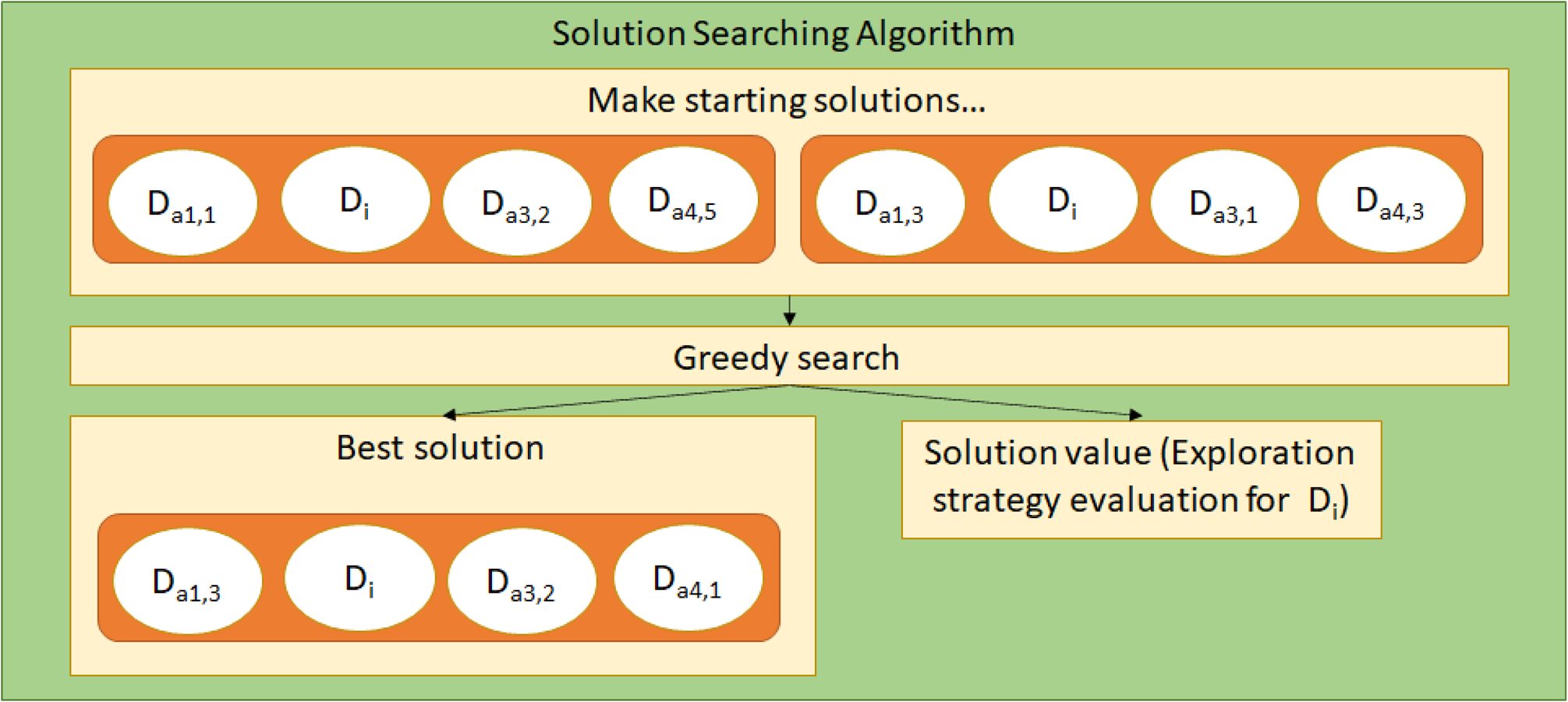
Figure 6 shows how new solutions are created from agents’ sets and evaluated to solve the minimization problem. An initial population of random solutions is first created using published designs, and designs within the solutions are changed according to a greedy algorithm. The best solution's value is then used as the f iint value. Agents do not have to search for new solutions at every iteration and instead may continue using the previously used solution to save resources. The integrating strategy finds the intersection of sets by discovering the best combinations of designs, measured by the project objective function of the solution they create. It also establishes feasibility by ensuring that designers stay within their sets; if a designer strays from its set and creates an incompatible design, then that design's evaluation becomes heavily penalized, resulting in the rejection of actions that make it incompatible.
Design problems
Design methodologies may be tested in various situations by simulating over different design problems. One key factor that is varied in these problems is the degree of coupling, indicating how much a design for one subproblem influences which designs for other subproblems are best. Other factors that change with problems are the difficulties of individual subproblems, and the number of agents to coordinate.
Model problem
A model problem allows a clear definition of coupled and uncoupled subobjectives to test the impacts of SBCE with different problems and numbers of agents. In this problem, the uncoupled subobjective promotes maximizing each agents’ dependent variables, while the coupled subobjective requires balancing these variables and their scaling factors. To make the problem simple and extendable, all agents control similarly structured variables. The agents manage two dependent variables each, defined as
Agent i: a i, b i, i = 1…n,
where a is the primary dependent variable and b is its scaling factor in the coupled subobjective. Dependent variables use the relations
 $$a_1 \ldots a_n = w_{1 \ldots n}\ast x_{1 \ldots n}, \;\,2\;< w_{1 \ldots n}, \;x_{1 \ldots n} < 10, \;$$
 $$\;b_1 \ldots b_n = y_{1 \ldots n}\ast z_{1 \ldots n}, \;0\;< y_{1 \ldots n}, \;z_{1 \ldots n} < 0.5, \;$$
where w 1…n, x 1…n, y 1…n, z 1…n are the independent variables. All variables are continuous and are changed by Eqs (9) and (10):
 $${\rm Continuous}\,{\rm Increase\colon }\;v_{new} = v_{old} + ( {v_{max}-v_{old}} ) \ast r; \;$$
 $${\rm Continuous\;}\,{\rm Decrease}\colon \;v_{new} = v_{old}-( {v_{old}-v_{min}} ) \ast r, \;$$
where v old is the pre-change value, v new is the post-change value, v max is the variable's upper limit, v min is the lower limit, and r is a uniform random number from 0 to 1.
The problem objective function for the model problem is defined as follows:
 $$f = f_u\ast w_u + f_c\ast w_c$$
 $$f_u = \mathop \sum \limits_1^n -a_n$$
 $$f_c = abs\left({a_1 + \mathop \sum \limits_2^n a_n\ast ( {b_1-b_n + 1.125} ) \ast {( {-1} ) }^{n-1}} \right)$$
where f u, f c are the uncoupled and coupled portions of the objective function, and w u, w c are their respective weights which allow the problem to transition between uncoupled and coupled. The coupled subobjective is made to avoid trivial solutions and allow the coordination of any number of agents. The ( − 1)n−1 factor ensures that agents are split evenly between positive and negative contributions to the sum, though odd numbers of agents will be slightly imbalanced. The (b 1 − b n + 1.125) term gives agents limited control over the scaling of their a n contributions. The constant of 1.125 is used to prevent the overall scale from becoming 1 or 0 at extreme values of b 1…b m, which would trivially solve the coupled subobjective by repeated use of Eqs (9) or (10).
The absolute value of a sum of variables controlled by different agents represents the need to finely balance different subproblem properties. Additionally, the primary dependent variable used in the coupled subproblem is also maximized for the uncoupled subproblem. This prevents agents from driving the relevant values down to their minimum to avoid the coupled subproblem and requires them to reconcile the two in a mixed case.
SAE car design problem
The contextual design problem used to verify the process in this work is the formula SAE car problem defined by Soria Zurita et al. (Reference Soria Zurita, Colby, Tumer, Hoyle and Tumer2018). This problem is chosen as it presents a large enough project to distribute among a design team while being simple enough to quickly evaluate for the simulator. Some roles in the previous work are merged to make each subproblem roughly equally complex. The new subproblems are given in Table 1.
Subproblems for the SAE car problem used in this work

Designs options consist of varying parameters for the architecture described in Soria Zurita et al. (Reference Soria Zurita, Colby, Tumer, Hoyle and Tumer2018) to create designs with different characteristics; these parameters are the independent variables in this work and include continuous variables such as part dimensions or locations and discrete variables such as material selection or catalogue selections for complex parts like engines. Continuous variables are changed by Eqs (9) and (10), while discrete variables are similarly changed with the following equations:
 $${\rm Discrete}\,{\rm Increase}\colon \;v_{new} = v_{old} + randint( {1, \;\;v_{max}-v_{old}} ) $$
 $${\rm Discrete}\,{\rm Decrease}\colon \;v_{new} = v_{old}-randint( {1, \;\;v_{old}-v_{min}} ) , \;$$
where the randint function returns a random integer between the given lower and upper bounds. Dependent variables include functional characteristics such as part masses, wing downforces, or tire radii.
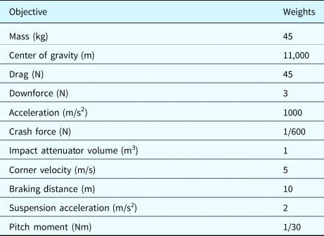
The problem objective function for the SAE car problem is a weighted sum of 12 factors. Factors to minimize are the car's mass, center of gravity, aerodynamic drag, crash force, impact attenuator volume, braking distance, suspension acceleration, and pitch moment. Factors to maximize are the car's aerodynamic downforce, acceleration, and corner velocity.
Weights between the subobjectives differ from Soria Zurita et al. (Reference Soria Zurita, Colby, Tumer, Hoyle and Tumer2018) to account for differences in the scales of subobjectives, which range from tenths to millions of units. Subobjectives are divided into primary and secondary subobjectives like the previous work. Primary subobjectives are the car's mass, center of gravity, drag, downforce, and acceleration. Secondary subobjectives are the crash force, impact attenuator volume, corner velocity, braking distance, suspension acceleration, and pitch moment. Weights are adjusted to make each primary and secondary subobjective contribute roughly equally to others in its group, with secondary subobjectives contributing less than primary subobjectives. The resulting weights are given in Table 2.
Weights of the SAE car subobjectives used in this work
The subobjectives of the SAE car problem are analyzed to generate a Design Structure Matrix as shown in Figure 7 to highlight subproblem dependencies and coupled systems. It is found that most subobjectives do not create significantly coupled subproblems as either subobjectives belonging to different subproblems are summed, allowing them to independently optimize, or dependencies are simple and only between two subproblems, such as subproblem 4 coupling only with subproblem 5 to balance the car's braking distance and acceleration, indicated by the lightly shaded box in Figure 7. Constraints also add some dependencies between subproblems, but these effects have minor influences on project development.
Design structure matrix of the SAE car problem. Constraining dependencies are marked with Xs. Subproblems 4 and 5 coupled through acceleration are lightly shaded, while subproblems coupled through pitch moment are more darkly shaded

The only significantly coupled subobjective identified is pitch moment, which is modified from the previous work by using an absolute value to minimize the moment in either direction. This necessitates coordination between all agents except subproblem 4 indicated by the darkly shaded box in Figure 7, as forces are positive or negative based on where they are positioned on the car and are scaled based on the cabin length and wing lengths. Due to the absolute value agents must balance relevant variables to reach 0 as closely as possible, similar to the model problem.
The pitch moment subobjective, by coupling five out of the six agents, presents an opportunity to easily vary the necessity of agent coordination in this problem by changing its weight. The default weighting, which considers it only a secondary subobjective and therefore weights it low, will behave as an uncoupled problem as agents favor optimizing primary subobjectives which do not require coordination. Increasing its weight such that it becomes significant, however, will make the problem behave as coupled, allowing testing of SBCE on both coupled and uncoupled contextualized problems.
While the SAE car problem uses a similar mechanism to couple agents, it is distinguished from the model problem by the difficulty of its uncoupled subobjectives, which are more numerous and have more complex relationships with their independent variables. This may change how SBCE impacts the uncoupled objective as it develops at a different rate. It is also more heterogeneous than the model problem, as each agent has a different degree of influence on the overall objective function and the coupled pitch moment subobjective; for example, the wing agents have significantly more influence on pitch moment than the cabin or suspension agents.
Experimental setup
All simulations are run for 1000 iterations to allow quality trends to settle, indicating rough project completion. Because these iterations are constant with respect to set size and are divided over designs in the sets, this also establishes an equal amount of development effort per project. Progress is also observed at shorter timespans to investigate shorter deadlines and lower-effort projects. Simulations are run 20 times for each condition and the results are averaged to account for the stochasticity of agents’ move selection, acceptance, and rejection. Rework is not conducted in these simulations, therefore projects that would otherwise require it are expected to perform poorly. Agents publish their designs every 20 iterations, and when using the integrating strategy, search for new solutions every 10 iterations where they reassess which designs to combine their own with during development. The objective function is minimized so results are presented as lower-is-better. In most cases the integrating strategy is used for the entire project; the investigation of the exploring strategy is conducted in a separate study only on the SAE car problem. The model problem is excluded from the exploration study due to its simplicity; each agent does not control enough variables to meaningfully use the exploring strategy.
Results and discussion
Model problem
Figure 8 investigates the performance of the model problem with respect to set size and weighting of uncoupled versus coupled objectives to test if SBCE can prevent rework and how applicable it is in various scenarios. The uncoupled model problem only considers its uncoupled subobjective, the coupled model problem only considers its coupled subobjective, and the mixed model problem considers both of them equally. The horizontal axis represents set sizes and therefore design candidates per set, while the number of sets is fixed by the problem itself. Each point on the vertical axis represents the best solution made from candidate designs from each set in a simulated project. Figure 8a displays the uncoupled case, with weight given to only the uncoupled objective; Figure 8b displays the mixed case, with equal weight to both, and Figure 8c displays the coupled case, with weight given only to the coupled objective. Y axes differ between these figures due to the different scales of relevant effects. Box plots are used as the data are skewed with long tails of lower-quality solutions. The box spans the 75th and 25th percentiles of the data, or upper and lower quartiles. The horizontal line in the box marks the data median. The whiskers extend to the nearest data points within 1.5 times the height of the box, or interquartile distance (IQD). All data points beyond this distance are marked as outliers with individual points. The many outlying points are due to the saturation of solutions at the problem's minimum objective function value of −600, causing small IQDs.
Project objective function values with respect to set size for the (a) uncoupled, (b) mixed, and (c) coupled model problems with six agents. Figures for other numbers of agents are given in the Appendix. Whiskers are +/1.5 IQD. Axes differ between figures due to the different scales of relevant effects.

Problems in Figure 8a, which focus only on the uncoupled subobjective, indicate that PBCE, corresponding to the set size of 1, performs better and more consistently than SBCE. SBCE's worse performance, in this case, can be explained by less time being devoted to each design, so they are less likely to reach the minimum. Problems in Figure 8c focus only on the coupled subobjective. In these, the trend is reversed where PBCE performs worse it cannot reliably coordinate agents to resolve the coupled subobjective. SBCE succeeds in coordinating the agents, with somewhat better performance at a set size of 2 and much better at 3 and greater. The mixed problem in Figure 8b shows results like those in Figure 8c as the coupled subobjective creates a larger difference than the uncoupled one. PBCE performs adequately much of the time in this case but has two extreme failures indicated by the outlying points at −560 and −470 quality, while SBCE does not show any similar failures. These severe failures in coupled cases result from failure to coordinate agents and reconcile the two subobjectives and would require restarting the project to achieve better performance. These failures correlate to the “dead end” designs in PBCE that require rework, corroborating arguments that SBCE reduces the need for rework in complex projects.
Figure 9 investigates the same simulations as Figure 8, but at shorter timescales to investigate the rate that SBCE progresses in the early phases of projects. To account for skew, median regression was used. The 75th percentile is also plotted to investigate if a process is frequently failing. Because the integrating strategy is used from the beginning of each project, no time is spent explicitly exploring the design space. For the uncoupled problem in Figure 9a, it is found that the trend of quality with respect to set size becomes significantly worse at shorter timespans (t(316) > 8.17, p < 0.001), supporting the statement that early phases of projects progress slowly in SBCE (Lycke, Reference Lycke2018). For the coupled problem in Figure 9c, this degradation is not observed. Instead, performance improves with increasing set size and improves even more at shorter timespans (t(316) > 3.35, p < 0.001), suggesting that shorter timespans magnify both PBCE's poor coordination of agents and SBCE's underdevelopment of uncoupled designs, as there is little time to compensate for process weaknesses with additional optimization. Figure 9b, presenting the mixed problem, clearly demonstrates both effects at 500 and 250 iterations. PBCE performs inconsistently due to its inability to coordinate agents for the coupled subobjective, with failures prevalent in the 75th percentiles. Large set sizes show gradual degradation of quality due to the underdevelopment of designs for the uncoupled subobjective. In this case, small set sizes perform the best as they coordinate agents while allowing them sufficient time to develop individual designs.
Solution objective function values with respect to subobjective weightings, set size, and elapsed time for the (a) uncoupled, (b) mixed, and (c) coupled model problems. Dark lines are sample medians, while light lines are 75th percentiles. Axes differ between figures due to the different scales of relevant effects.

SAE car problem
Figure 10 shows how the SAE car project performs over different set sizes and weightings of the pitch moment subobjective, presenting effects on the contextualized problem with varying degrees of coupling. The uncoupled problem in Figure 10a uses the default pitch moment weighting, the mixed problem in Figure 10b uses 100× weighting, and the coupled problem in Figure 10c 1000× weighting. For the uncoupled problem in Figure 10a, results are like those in Figure 8a, where a trend of gradually decreasing quality with set size is observed (t(158) = 6.052, p < 0.001). Figure 10b presents the mixed problem. Here PBCE and the set size of 2 show bimodal distributions, indicating “success” and “failure” cases. This bimodal distribution transitions to a more normal distribution at set sizes 3 and higher, indicating resolution of agent coordination; however, overall quality also decreases as set size further increases (t(158) = 4.359, p < 0.001). This simultaneously demonstrates the failure to coordinate agents in PBCE, and inefficiency due to dividing time among designs in SBCE. The highly coupled case in Figure 10c shows that PBCE fails to coordinate agents even more frequently, while SBCE successfully does so at any set size. These results indicate that results from the model problem generalize to contextualized problems. Additionally, small set sizes around 3 perform similarly to PBCE on uncoupled problems while also succeeding in coupled problems, suggesting that SBCE should be widely applicable in problems of unknown structure.
Solution objective function values for different pitch moment weightings on the SAE car problem. (a) represents low weightings, (b) intermediate weightings, and (c) high weightings of the coupled subobjective, respectively. Whiskers are +/1.5 IQD (c) uses a different axis due to the large value at set size of 1.

Figure 11 investigates the previous results at shorter timespans similar to Figure 9. Performance with respect to set size continues to worsen at short timespans as in the model problem but to a lesser degree. For the uncoupled SAE car problem in Figure 11(a), the only significant difference is between 1000 and 500 iterations (t(316) = 4.52, p < 0.001). In the mixed problem in Figure 11b, significant differences are observed with respect to 1000 iterations (t(316) > 2.43, p = 0.015), but not between 250 and 500 iterations (t(316) = 0.854, p = 0.39). In the highly coupled problem in Figure 11c, only 250 iterations show significant differences between other timespans (t(316) > 2.60, p < 0.010). While these results are weaker, they continue to suggest that large set sizes perform especially worse on short projects, lending further credibility to the statement that SBCE projects often have slow starts (Lycke, Reference Lycke2018). Small set sizes continue to perform well while mitigating difficulties on coupled subobjectives, however, promising a solution to this dilemma.
Solution objective function values with respect to pitch moment weight, set size, and elapsed time on the SAE car problem. (a) represents low weightings, (b) intermediate weightings, and (c) high weightings of the coupled subobjective, respectively. Dark lines are sample medians, while light lines are 75th percentiles. (c) uses a different axis due to the large values at set size of 1.

Design exploration impacts
Figure 12 further investigates the slow start of projects in SBCE by considering the cost of time spent mapping the design space. In this figure, projects are given 1000 total iterations, divided between exploration and integration. The default SAE car subobjective weightings are used, and the PBCE case is omitted as it lacks the multiple designs needed to use the exploring strategy well. Most projects perform worse if they spend time exploring (t(316) > 2.54, p < 0.011); however, there is little difference between the cases that do explore. When 100% of the time is spent exploring, projects frequently perform poorly, indicated by the upper quartile line, as they do not explicitly optimize for the project. Large set sizes mitigate this as the design space is more thoroughly explored, however. These losses in performance due to exploration are because the exploring strategy does not directly solve the problem's objective function. Such a misalignment is unavoidable, as the precise priorities for designs are unknown until the time is devoted to making an integrated solution which requires using the integrating strategy. This loss in performance, therefore, suggests that taking time to explore the design space and generate knowledge contributes to the slow start of projects in SBCE.
Solution objective function values for a project with 1000 total iterations using the default weights, divided between exploration and integration. Dark lines are sample medians, while light lines are 75th percentiles.

While design space exploration may contribute to the slow start of a project, a key practice in SBCE is reusing that exploration and its generated knowledge for future projects. Designs created using the exploring strategy can represent pre-existing knowledge, as they are generally useful but are not aligned with the specific project being developed. In this case, exploration has already been completed, and so does not detract from integration. Figure 13 presents the impacts of varying amounts of exploration on the SAE car problem at different timespans of integration to test the benefits of design capture and reuse. Exploration significantly improves project performance at all timespans and set sizes (t(158) > 2.80, p < 0.006), and becomes especially important for very short projects as in the 250 iterations case (t(316) > 3.70, p < 0.003). These performance gains can be explained as generic designs created when mapping the design space, which may occur in previous projects, are carried over and reused to get a head start on new projects which allows them to create good solutions much faster.
Solution objective function values with respect to exploration iterations at different timespans in integration and set sizes of (a) two, (b) four, and (c) seven. Dark lines are sample medians, while light lines are 75th percentiles.

Conclusion
This work introduces the PSORT platform to simulate the SBCE process and its impacts on a design project. PSORT reproduces the chance for PBCE to fail on coupled problems, correlating to dead-end projects that require rework. These failures are mitigated or absent when simulating SBCE, reproducing its proposed stability. Additionally, it lends plausibility to concerns about dividing designers’ time over designs as uncoupled projects perform worse with large set sizes, though small set sizes perform adequately on uncoupled problems while consistently resolving coupled ones as well, supporting statements of SBCE's wide applicability except in very simple, short projects in Raudberget (Reference Raudberget2010). Other effects reproduced include the slow start on projects observed in Lycke (Reference Lycke2018), and the benefits of recording and reusing designs in future projects. The reproduction of all these effects when implementing the principles of SBCE suggests the applicability of this platform to further study the impacts of SBCE on new team and problem structures.
While the simulated projects lend plausibility to concerns about the inefficiency of developing many designs throughout the project, a conservative approach in which small sets are used, combined with a focus on creating an integrated solution from the beginning, is found to mitigate this inefficiency while still performing well on coupled problems. Therefore, it may be desired to use SBCE to mitigate potential difficulties when the coupling of the problem is uncertain.
SBCE's principle of mapping the design space may significantly contribute to the slow start of projects, as designers must first devote time to learning the capabilities of their discipline and how they interact with others. The knowledge and designs generated from this process can be reused in future projects to significantly improve performance under tight schedules, however. This highlights how mapping the design space allows future projects to be completed much more efficiently, despite its upfront costs.
Future work includes expanding on the limitations of PSORT to explore how SBCE interacts with other aspects of design team composition. PSORT currently requires that only one agent works on each subproblem, presenting an opportunity for SBCE to coordinate multiple agents assigned to a single subproblem in new ways. Another limitation is that only one decomposition of the SAE car problem is used, leaving open further investigation of how SBCE's benefits to coordination interact with other degrees of problem decomposition. Modeling with more complex and varied agents may investigate how agent properties and communication influence the process. Finally, the use of other solving methods during iteration may allow for new insights and explicit modeling of other factors such as uncertainty.
Acknowledgements
The authors would like to thank Mitchell Fogelson and Ambrosio Valencia-Romero for their review and comments on this work. This work was partially supported by the Defense Advanced Research Projects Agency through cooperative agreement N66001-17-1-4064. Any opinions, findings, and conclusions or recommendations expressed in this paper are those of the authors and do not necessarily reflect the views of the sponsors.
Software availability
The simulator source code used for this study is openly available in the SBCE-Simulator repository at http://doi.org/referencenumber10.5281/zenodo.7048666.
Competing interests
The authors declare no competing interests.
Sean Rismiller received his PhD in mechanical engineering from Carnegie Mellon University where he used simulation to research how the engineering design process is influenced by various conditions. He conducted further simulation research using molecular dynamics simulations to study chemical reactions at the University of Missouri - Columbia, where he received his bachelor's in mechanical engineering.
Jonathan Cagan is the David and Susan Coulter Head of Mechanical Engineering and George Tallman and Florence Barrett Ladd Professor at Carnegie Mellon University, with an appointment in Design. Cagan also served as Interim Dean of the College of Engineering and Special Advisor to the Provost. Cagan co-founded the Integrated Innovation Institute for interdisciplinary design education at CMU, bringing engineering, design and business together to create new products and services. Cagan's research focuses on design automation and methods, problem solving, and medical technologies. His work merges AI, machine learning, and optimization methods with cognitive- and neuro-science problem solving. A Fellow of the American Society of Mechanical Engineers, Cagan has been awarded the ASME Design Theory and Methodology, Design Automation, and Ruth and Joel Spira Outstanding Design Educator Awards. He is also a Fellow of the American Association for the Advancement of Science.
Christopher McComb is a faculty member in Carnegie Mellon University's Department of Mechanical Engineering. Previously, he was an assistant professor in the School of Engineering Design, Technology, and Professional Programs at Penn State. He also served as director of Penn State's Center for Research in Design and Innovation and led its Technology and Human Research in Engineering Design Group. He received dual B.S. degrees in civil and mechanical engineering from California State University-Fresno. He later attended Carnegie Mellon University as a National Science Foundation Graduate Research Fellow, where he obtained his M.S. and Ph.D. in mechanical engineering. His research interests include human social systems in design and engineering; machine learning for engineering design; human-AI collaboration and teaming; and STEM education, with funding from NSF, DARPA, and private corporations.
Appendix
Trends of solution quality with respect to set size were found to be similar over the number of agents present. Demonstration of this is shown in Figure A1 for both 3 and 4 agents, demonstrating similar cases for both even and odd numbers of agents.
Solution objective function values with respect to set size for the model problem for three (A,B,C) and four (D,E,F) agents. U represents the weight of the uncoupled objective, and C represents the weight of the coupled objective. Error bars are +/1 SE Axes that differ between figures due to the different scales of relevant effects.


 Open access