


1. Introduction ${\mathrm{HESS\,J}1804{-}216}$
is one of the brightest unidentified
${\mathrm{HESS\,J}1804{-}216}$
is one of the brightest unidentified ${\gamma}$
-ray sources, discovered by the High Energy Stereoscopic System (H.E.S.S.) in 2004 as part of the first H.E.S.S. Galactic Plane Survey (Aharonian et al. Reference Aharonian2005).
${\gamma}$
-ray sources, discovered by the High Energy Stereoscopic System (H.E.S.S.) in 2004 as part of the first H.E.S.S. Galactic Plane Survey (Aharonian et al. Reference Aharonian2005). ${\mathrm{HESS\,J}1804{-}216}$
features extended emission with a radius of
${\mathrm{HESS\,J}1804{-}216}$
features extended emission with a radius of ${\mathord{\sim}22\,{\rm arcmin}}$
, a photon flux of almost 25% of the Crab Nebula above 200 GeV (Aharonian et al. Reference Aharonian2006), and a TeV luminosity of
${\mathord{\sim}22\,{\rm arcmin}}$
, a photon flux of almost 25% of the Crab Nebula above 200 GeV (Aharonian et al. Reference Aharonian2006), and a TeV luminosity of ${5\times10^{33}(\rm d/kpc)^2\,\mathrm{erg\,s^{-1}}}$
and is one of the softest galactic sources with a photon index of
${5\times10^{33}(\rm d/kpc)^2\,\mathrm{erg\,s^{-1}}}$
and is one of the softest galactic sources with a photon index of ${\Gamma = 2.69\,{\pm}\,0.04}$
(H.E.S.S. Collaboration et al. Reference Collaboration2018a).
${\Gamma = 2.69\,{\pm}\,0.04}$
(H.E.S.S. Collaboration et al. Reference Collaboration2018a).
High-Altitude Water Cherenkov observatory (HAWC) detected emission at ${\mathord{\sim}4\sigma}$
towards the north of
${\mathord{\sim}4\sigma}$
towards the north of ${\mathrm{HESS\,J}1804{-}216}$
; however, no source has been identified.
${\mathrm{HESS\,J}1804{-}216}$
; however, no source has been identified.
The GeV ${\gamma}$
-ray source,
${\gamma}$
-ray source, ${\mathrm{FGES\,J}1804.8{-}2144}$
, (Ackermann et al. Reference Ackermann2017) is a disc of radius
${\mathrm{FGES\,J}1804.8{-}2144}$
, (Ackermann et al. Reference Ackermann2017) is a disc of radius ${\mathord{\sim}23\ {\rm arcmin}}$
, coincident with the TeV emission from
${\mathord{\sim}23\ {\rm arcmin}}$
, coincident with the TeV emission from ${\mathrm{HESS\,J}1804{-}216}$
(see Figure 1).
${\mathrm{HESS\,J}1804{-}216}$
(see Figure 1). ${\mathrm{HESS\,J}1804{-}216}$
has several possible counterparts found within
${\mathrm{HESS\,J}1804{-}216}$
has several possible counterparts found within ${\mathord{\sim}1^{\circ}}$
of its centroid, but none of these have been unambiguously associated with the TeV source. Two prominent candidates for the acceleration of cosmic rays (CRs) are supernova remnants (SNRs) and pulsar wind nebulae (PWNe). Here, the potential counterparts are
${\mathord{\sim}1^{\circ}}$
of its centroid, but none of these have been unambiguously associated with the TeV source. Two prominent candidates for the acceleration of cosmic rays (CRs) are supernova remnants (SNRs) and pulsar wind nebulae (PWNe). Here, the potential counterparts are ${\mathrm{SNR\,G}8.7{-}0.1}$
,
${\mathrm{SNR\,G}8.7{-}0.1}$
, ${\mathrm{SNR}\,8.3{-}0.1}$
(also referred to as SNR G8.3
${\mathrm{SNR}\,8.3{-}0.1}$
(also referred to as SNR G8.3 ${-}$
0.0 in other literature, see Hewitt & Yusef-Zadeh Reference Hewitt and Yusef-Zadeh2009),
${-}$
0.0 in other literature, see Hewitt & Yusef-Zadeh Reference Hewitt and Yusef-Zadeh2009), ${\mathrm{PSR\,J}1803{-}2137}$
,
${\mathrm{PSR\,J}1803{-}2137}$
, ${\mathrm{PSR\,J}1803{-}2149}$
, and PSR J1806
${\mathrm{PSR\,J}1803{-}2149}$
, and PSR J1806 ${-2125}$
. The location of each counterpart with respect to
${-2125}$
. The location of each counterpart with respect to ${\mathrm{HESS\,J}1804{-}216}$
is shown in Figure 1. The
${\mathrm{HESS\,J}1804{-}216}$
is shown in Figure 1. The ${\gamma}$
-ray contours used here were obtained from Aharonian et al. (Reference Aharonian2006).
${\gamma}$
-ray contours used here were obtained from Aharonian et al. (Reference Aharonian2006). ${\mathrm{SNR}\,8.3{-}0.1}$
has radio shell-like morphology with a radius of
${\mathrm{SNR}\,8.3{-}0.1}$
has radio shell-like morphology with a radius of ${0.04^{\circ}}$
(Kilpatrick, Bieging, & Rieke Reference Kilpatrick, Bieging and Rieke2016; Acero et al. Reference Acero2016). Kilpatrick et al. (Reference Kilpatrick, Bieging and Rieke2016) find a systematic velocity of
${0.04^{\circ}}$
(Kilpatrick, Bieging, & Rieke Reference Kilpatrick, Bieging and Rieke2016; Acero et al. Reference Acero2016). Kilpatrick et al. (Reference Kilpatrick, Bieging and Rieke2016) find a systematic velocity of ${+2.6\,\,\mathrm{km\,s}^{-1}}$
, placing it at a kinematic distance of 16.4 kpc, hence it is in the background.
${+2.6\,\,\mathrm{km\,s}^{-1}}$
, placing it at a kinematic distance of 16.4 kpc, hence it is in the background. ${\mathrm{SNR}\,8.3{-}0.1}$
would have an unusually high TeV luminosity (H.E.S.S. Collaboration et al. Reference Collaboration2018a) at 16.4 kpc of
${\mathrm{SNR}\,8.3{-}0.1}$
would have an unusually high TeV luminosity (H.E.S.S. Collaboration et al. Reference Collaboration2018a) at 16.4 kpc of ${1.34\times10^{36}\,\mathrm{erg\,s}^{-1}}$
, making it unlikely to be powering
${1.34\times10^{36}\,\mathrm{erg\,s}^{-1}}$
, making it unlikely to be powering ${\mathrm{HESS\,J}1804{-}216}$
.
${\mathrm{HESS\,J}1804{-}216}$
. ${\mathrm{SNR\,G}8.7{-}0.1}$
has a large radius of
${\mathrm{SNR\,G}8.7{-}0.1}$
has a large radius of ${26 {\rm arcmin}}$
as determined by radio observations (Fang & Zhang Reference Fang and Zhang2008). It has been associated with a number of young Hii regions, forming the W30 complex, a large star-forming region with a
${26 {\rm arcmin}}$
as determined by radio observations (Fang & Zhang Reference Fang and Zhang2008). It has been associated with a number of young Hii regions, forming the W30 complex, a large star-forming region with a ${\mathord{\sim}1^{\circ}}$
region of radio continuum emission (Kassim & Weiler Reference Kassim and Weiler1990).
${\mathord{\sim}1^{\circ}}$
region of radio continuum emission (Kassim & Weiler Reference Kassim and Weiler1990). ${\mathrm{SNR\,G}8.7{-}0.1}$
is a mature SNR with an age of 15 kyr (Odegard Reference Odegard1986). A distance of 4.5 kpc is adopted here, which is found through X-ray observations and the column density of neutral hydrogen (Hewitt & Yusef-Zadeh Reference Hewitt and Yusef-Zadeh2009). Ajello et al. (Reference Ajello2012) modelled the GeV to TeV emission assuming CRs are accelerated by this SNR.
${\mathrm{SNR\,G}8.7{-}0.1}$
is a mature SNR with an age of 15 kyr (Odegard Reference Odegard1986). A distance of 4.5 kpc is adopted here, which is found through X-ray observations and the column density of neutral hydrogen (Hewitt & Yusef-Zadeh Reference Hewitt and Yusef-Zadeh2009). Ajello et al. (Reference Ajello2012) modelled the GeV to TeV emission assuming CRs are accelerated by this SNR.
A 1720-MHz OH is located along the southern edge of ${\mathrm{SNR\,G}8.7{-}0.1}$
(Hewitt & Yusef-Zadeh Reference Hewitt and Yusef-Zadeh2009). It is currently categorised as an SNR-type maser, as no compact radio source has been found within
${\mathrm{SNR\,G}8.7{-}0.1}$
(Hewitt & Yusef-Zadeh Reference Hewitt and Yusef-Zadeh2009). It is currently categorised as an SNR-type maser, as no compact radio source has been found within ${5\ {\rm arcmin}}$
and it is believed to originate in a post-shock environment (Fernandez et al. Reference Fernandez2013). It is located at a velocity (
${5\ {\rm arcmin}}$
and it is believed to originate in a post-shock environment (Fernandez et al. Reference Fernandez2013). It is located at a velocity ( ${\mathrm{v}_{\mathrm{lsr}}}$
) of
${\mathrm{v}_{\mathrm{lsr}}}$
) of ${36\,\mathrm{km\,s}^{-1}}$
corresponding to a distance of
${36\,\mathrm{km\,s}^{-1}}$
corresponding to a distance of ${\mathord{\sim}4.55}$
kpc, similar to the distance to
${\mathord{\sim}4.55}$
kpc, similar to the distance to ${\mathrm{SNR\,G}8.7{-}0.1}$
. The coexistence of molecular clouds with
${\mathrm{SNR\,G}8.7{-}0.1}$
. The coexistence of molecular clouds with ${\mathrm{SNR\,G}8.7{-}0.1}$
and the location of the OH maser suggest that the SNR is interacting with nearby molecular clouds (Hewitt & Yusef-Zadeh Reference Hewitt and Yusef-Zadeh2009).
${\mathrm{SNR\,G}8.7{-}0.1}$
and the location of the OH maser suggest that the SNR is interacting with nearby molecular clouds (Hewitt & Yusef-Zadeh Reference Hewitt and Yusef-Zadeh2009).
The characteristics of the pulsars are summarised in Table 1. ${\mathrm{PSR\,J}1803{-}2137}$
was found by high-frequency radio observations by Clifton & Lyne (Reference Clifton and Lyne1986). A dispersion measure distance of 3.8 kpc is used here (Kargaltsev, Pavlov, & Garmire Reference Kargaltsev, Pavlov and Garmire2007a). Chandra detected a faint and small (
${\mathrm{PSR\,J}1803{-}2137}$
was found by high-frequency radio observations by Clifton & Lyne (Reference Clifton and Lyne1986). A dispersion measure distance of 3.8 kpc is used here (Kargaltsev, Pavlov, & Garmire Reference Kargaltsev, Pavlov and Garmire2007a). Chandra detected a faint and small ( ${\mathord{\sim}7\ {\rm arcsec} \times4\ {\rm arcsec}}$
) synchrotron nebula around
${\mathord{\sim}7\ {\rm arcsec} \times4\ {\rm arcsec}}$
) synchrotron nebula around ${\mathrm{PSR\,J}1803{-}2137}$
, with the inner PWN positioned perpendicular to the direction of proper motion of the pulsar (Kargaltsev et al. Reference Kargaltsev, Pavlov and Garmire2007a).
${\mathrm{PSR\,J}1803{-}2137}$
, with the inner PWN positioned perpendicular to the direction of proper motion of the pulsar (Kargaltsev et al. Reference Kargaltsev, Pavlov and Garmire2007a).
Pulsar characteristics, including spin period (P), period derivative ( ${\dot{P}}$
), characteristic age (
${\dot{P}}$
), characteristic age ( ${\tau_c}$
), spin-down power (
${\tau_c}$
), spin-down power ( ${\dot{E}}$
), distance, and TeV luminosity at that distance.
${\dot{E}}$
), distance, and TeV luminosity at that distance.

aFrom Brisken et al. (Reference Brisken, Carrillo-Barragán, Kurtz and Finley2006).
bFrom Abdo et al. (Reference Abdo2013).
cFrom Morris et al. (Reference Morris2002).
TeV ${\gamma}$
-ray significance map of
${\gamma}$
-ray significance map of ${\text{HESS\,J}1804{-}216}$
, along with potential counterparts.
${\text{HESS\,J}1804{-}216}$
, along with potential counterparts. ${\text{SNR\,G}8.7{-}0.1}$
and
${\text{SNR\,G}8.7{-}0.1}$
and ${\text{SNR}\,8.3{-}0.1}$
are indicated by the blue dashed circles,
${\text{SNR}\,8.3{-}0.1}$
are indicated by the blue dashed circles, ${\text{PSR\,J}1803{-}2137}$
,
${\text{PSR\,J}1803{-}2137}$
, ${\text{PSR\,J}1803{-}2149}$
, and PSR J1806
${\text{PSR\,J}1803{-}2149}$
, and PSR J1806 ${-2125}$
are indicated by the white dots and the 1720-MHz OH is indicated by a purple cross.
${-2125}$
are indicated by the white dots and the 1720-MHz OH is indicated by a purple cross. ${\text{FGES\,J}1804.8{-}2144}$
is shown by the yellow dashed circle. The TeV
${\text{FGES\,J}1804.8{-}2144}$
is shown by the yellow dashed circle. The TeV ${\gamma}$
-ray emission for 5-10
${\gamma}$
-ray emission for 5-10 ${\sigma}$
is shown by the solid white contours. Image adapted from H.E.S.S. Collaboration et al. (Reference Collaboration2018a).
${\sigma}$
is shown by the solid white contours. Image adapted from H.E.S.S. Collaboration et al. (Reference Collaboration2018a).
 ${\mathrm{PSR\,J}1803{-}2137}$
is located towards the north-eastern edge of
${\mathrm{PSR\,J}1803{-}2137}$
is located towards the north-eastern edge of ${\mathrm{SNR\,G}8.7{-}0.1}$
, but their association is highly unlikely according to a proper motion study of the pulsar (Brisken et al. Reference Brisken, Carrillo-Barragán, Kurtz and Finley2006). This study showed that for the pulsar to be born at the centre of
${\mathrm{SNR\,G}8.7{-}0.1}$
, but their association is highly unlikely according to a proper motion study of the pulsar (Brisken et al. Reference Brisken, Carrillo-Barragán, Kurtz and Finley2006). This study showed that for the pulsar to be born at the centre of ${\mathrm{SNR\,G}8.7{-}0.1}$
, a transverse velocity of
${\mathrm{SNR\,G}8.7{-}0.1}$
, a transverse velocity of ${\mathord{\sim}1700\,\mathrm{km\,s}^{-1}}$
is required. Therefore,
${\mathord{\sim}1700\,\mathrm{km\,s}^{-1}}$
is required. Therefore, ${\mathrm{PSR\,J}1803{-}2137}$
was born outside the central region of
${\mathrm{PSR\,J}1803{-}2137}$
was born outside the central region of ${\mathrm{SNR\,G}8.7{-}0.1}$
(see Figure A1). The pulsar is most likely moving towards this area, rather than away from it, ruling out their connection (Brisken et al. Reference Brisken, Carrillo-Barragán, Kurtz and Finley2006).
${\mathrm{SNR\,G}8.7{-}0.1}$
(see Figure A1). The pulsar is most likely moving towards this area, rather than away from it, ruling out their connection (Brisken et al. Reference Brisken, Carrillo-Barragán, Kurtz and Finley2006).
PSR J1806 ${-2125}$
is a
${-2125}$
is a ${\gamma}$
-ray-quiet radio pulsar discovered with the Parkes radio telescope (Morris et al. Reference Morris2002), and is located at a distance of
${\gamma}$
-ray-quiet radio pulsar discovered with the Parkes radio telescope (Morris et al. Reference Morris2002), and is located at a distance of ${\mathord{\sim}10}$
kpc. Comparing the inferred
${\mathord{\sim}10}$
kpc. Comparing the inferred ${\gamma}$
-ray luminosity at 10 kpc to the spin-down power, we obtain a TeV
${\gamma}$
-ray luminosity at 10 kpc to the spin-down power, we obtain a TeV ${\gamma}$
-ray efficiency (
${\gamma}$
-ray efficiency ( ${\eta_{\gamma}=L_{\gamma}/\dot{E}}$
) of more than 100%, excluding it as a plausible counterpart.
${\eta_{\gamma}=L_{\gamma}/\dot{E}}$
) of more than 100%, excluding it as a plausible counterpart. ${\mathrm{PSR\,J}1803{-}2149}$
is a radio-quiet
${\mathrm{PSR\,J}1803{-}2149}$
is a radio-quiet ${\gamma}$
-ray pulsar located at a distance of 1.3 kpc (Pletsch et al. Reference Pletsch2012). This distance is obtained by inverting the
${\gamma}$
-ray pulsar located at a distance of 1.3 kpc (Pletsch et al. Reference Pletsch2012). This distance is obtained by inverting the ${\gamma}$
-ray luminosity equation (see Saz Parkinson et al. Reference Saz Parkinson2010) and is discussed further in Section 5.1.
${\gamma}$
-ray luminosity equation (see Saz Parkinson et al. Reference Saz Parkinson2010) and is discussed further in Section 5.1.
Multiple studies (Higashi et al. Reference Higashi2008; Kargaltsev, Pavlov, & Garmire Reference Kargaltsev, Pavlov and Garmire2007b; Lin, Webb, & Barret Reference Lin, Webb and Barret2013) have found a lack of X-ray emission towards ${\mathrm{HESS\,J}1804{-}216}$
, particularly towards
${\mathrm{HESS\,J}1804{-}216}$
, particularly towards ${\mathrm{SNR\,G}8.7{-}0.1}$
and
${\mathrm{SNR\,G}8.7{-}0.1}$
and ${\mathrm{PSR\,J}1803{-}2137}$
. As mentioned previously, there is a faint and small X-ray nebula towards
${\mathrm{PSR\,J}1803{-}2137}$
. As mentioned previously, there is a faint and small X-ray nebula towards ${\mathrm{PSR\,J}1803{-}2137}$
. No SNR shell has been detected within the field of view of the Chandra imaging (Kargaltsev et al. Reference Kargaltsev, Pavlov and Garmire2007b). Investigation of this region by XMM-Newton (Lin et al. Reference Lin, Webb and Barret2013) showed that the detected X-ray sources (both extended and point-like) are unlikely to be associated with
${\mathrm{PSR\,J}1803{-}2137}$
. No SNR shell has been detected within the field of view of the Chandra imaging (Kargaltsev et al. Reference Kargaltsev, Pavlov and Garmire2007b). Investigation of this region by XMM-Newton (Lin et al. Reference Lin, Webb and Barret2013) showed that the detected X-ray sources (both extended and point-like) are unlikely to be associated with ${\mathrm{HESS\,J}1804{-}216}$
due to them being located far away from the TeV peak.
${\mathrm{HESS\,J}1804{-}216}$
due to them being located far away from the TeV peak.
Our detailed arcminute-scale ISM study here follows on from earlier work by de Wilt et al. (Reference de Wilt2017) who revealed dense clumpy gas using the ammonia inversion line tracer. By studying the distribution and density of the ISM towards ${\mathrm{HESS\,J}1804{-}216}$
on arcminute scales, we can investigate morphological differences between hadronic and leptonic scenarios for the
${\mathrm{HESS\,J}1804{-}216}$
on arcminute scales, we can investigate morphological differences between hadronic and leptonic scenarios for the ${\gamma}$
-ray production. We will utilise data from the Mopra radio telescope and Southern Galactic Plane Survey (SGPS) in order to carry out such an investigation and look at an isotropic CR diffusion model for further insight into the likelihood of a hadronic interpretation.
${\gamma}$
-ray production. We will utilise data from the Mopra radio telescope and Southern Galactic Plane Survey (SGPS) in order to carry out such an investigation and look at an isotropic CR diffusion model for further insight into the likelihood of a hadronic interpretation.
2. ISM observations
In this work, we utilised the publicly available SGPS
Footnote a
of atomic hydrogen (HI) and 3, 7, and 12 mm (frequency ranges 76–117, 30–50, and 16–27 GHz, respectively) data taken with the Mopra radio telescope towards the ${\mathrm{HESS\,J}1804{-}216}$
region.
${\mathrm{HESS\,J}1804{-}216}$
region.
The Australia Telescope Compact Array (ATCA) and Parkes telescope together mapped the HI emission along the Galactic Plane to form the SGPS. The survey is for latitudes of ${b=\pm1.5^{\circ}}$
and longitudes covering
${b=\pm1.5^{\circ}}$
and longitudes covering ${l=253^{\circ}}$
–
${l=253^{\circ}}$
– ${358^{\circ}}$
(SGPS I) as well as
${358^{\circ}}$
(SGPS I) as well as ${l=5^{\circ}}$
–
${l=5^{\circ}}$
– ${20^{\circ}}$
(SGPS II, McClure-Griffiths et al. Reference McClure-Griffiths, Dickey, Gaensler, Green, Haverkorn and Strasser2005).
${20^{\circ}}$
(SGPS II, McClure-Griffiths et al. Reference McClure-Griffiths, Dickey, Gaensler, Green, Haverkorn and Strasser2005).
Mopra is a single dish with a 22-m diameter surface. The 3-mm data were taken from the Mopra SGPS, which is designed to map the fourth quadrant in the CO isotopologues (e.g. Braiding et al. Reference Braiding2018
Footnote b
). The Mopra spectrometer (MOPS) was used in wide-band mode at 8 GHz in Fast-On-The-Fly (FOTF) mapping to detect the four isotopologue lines ( ${^{12}\mathrm{CO}}$
,
${^{12}\mathrm{CO}}$
, ${^{13}\mathrm{CO}}$
,
${^{13}\mathrm{CO}}$
, ${\mathrm{C}^{17}}$
O, and
${\mathrm{C}^{17}}$
O, and ${\mathrm{C}^{18}}$
O). FOTF mapping is conducted by scanning across 1 square degree segments. To reduce artefacts in the data, each segment contains a longitudinal and latitudinal scan. The target region covering
${\mathrm{C}^{18}}$
O). FOTF mapping is conducted by scanning across 1 square degree segments. To reduce artefacts in the data, each segment contains a longitudinal and latitudinal scan. The target region covering ${\mathrm{HESS\,J}1804{-}216}$
is
${\mathrm{HESS\,J}1804{-}216}$
is ${b=\pm 0.5^{\circ}}$
and
${b=\pm 0.5^{\circ}}$
and ${l=7.0}$
–
${l=7.0}$
– ${9.0^{\circ}}$
for the two CO isotopologue lines of interest:
${9.0^{\circ}}$
for the two CO isotopologue lines of interest: ${^{12}\mathrm{CO}}$
and
${^{12}\mathrm{CO}}$
and ${^{13}\mathrm{CO}}$
.
${^{13}\mathrm{CO}}$
.
The 7-mm studies towards ${\mathrm{HESS\,J}1804{-}216}$
were taken in 2011 and 2012. The 7-mm coverage is for a
${\mathrm{HESS\,J}1804{-}216}$
were taken in 2011 and 2012. The 7-mm coverage is for a ${49 \times 52}$
arcmin region centred on
${49 \times 52}$
arcmin region centred on ${l=8.45^{\circ}}$
and
${l=8.45^{\circ}}$
and ${b=-0.07^{\circ}}$
. MOPS was used in ‘zoom’ mode for these observations. This provides 16 different subbands each with 4096 channels and a bandwidth of 137.5 MHz (Urquhart et al. Reference Urquhart2010). Table F.1 lists the various spectral lines at 7 mm.
${b=-0.07^{\circ}}$
. MOPS was used in ‘zoom’ mode for these observations. This provides 16 different subbands each with 4096 channels and a bandwidth of 137.5 MHz (Urquhart et al. Reference Urquhart2010). Table F.1 lists the various spectral lines at 7 mm.
The 12-mm receiver on the Mopra telescope was used to carry out the ${\mathrm{H}_2\mathrm{O}}$
SGPS (Walsh et al. Reference Walsh2011, HOPS). This survey also detected other molecules such as the different inversion transitions of ammonia (
${\mathrm{H}_2\mathrm{O}}$
SGPS (Walsh et al. Reference Walsh2011, HOPS). This survey also detected other molecules such as the different inversion transitions of ammonia ( ${\mathrm{NH}_3}$
). HOPS utilised On-The-Fly (OTF) mode with the Mopra wide-bandwidth spectrometer. HOPS mapped the region surrounding
${\mathrm{NH}_3}$
). HOPS utilised On-The-Fly (OTF) mode with the Mopra wide-bandwidth spectrometer. HOPS mapped the region surrounding ${\mathrm{HESS\,J}1804{-}216}$
;
${\mathrm{HESS\,J}1804{-}216}$
; ${b=\pm 0.5^{\circ}}$
and
${b=\pm 0.5^{\circ}}$
and ${l=7.0^{\circ}}$
–
${l=7.0^{\circ}}$
– ${9.0^{\circ}}$
.
${9.0^{\circ}}$
.
The Mopra 3-, 7-, and 12-mm data must be corrected to account for the extended beam efficiency of Mopra before any data analysis can be performed. The main beam brightness temperature is obtained by dividing the antenna temperature by the extended beam efficiency ( ${\eta_{XB}}$
). At 3 mm (115 GHz), for the CO(1-0) lines (
${\eta_{XB}}$
). At 3 mm (115 GHz), for the CO(1-0) lines ( ${^{12}\mathrm{CO}}$
and
${^{12}\mathrm{CO}}$
and ${^{13}\mathrm{CO}}$
), a value of
${^{13}\mathrm{CO}}$
), a value of ${\eta_{XB} = 0.55}$
(Ladd et al. Reference Ladd, Purcell, Wong and Robertson2005) is used. Following Urquhart et al. (Reference Urquhart2010), the 7-mm data are corrected to account for the beam efficiency of each frequency from Table F.1. At 12 mm for the
${\eta_{XB} = 0.55}$
(Ladd et al. Reference Ladd, Purcell, Wong and Robertson2005) is used. Following Urquhart et al. (Reference Urquhart2010), the 7-mm data are corrected to account for the beam efficiency of each frequency from Table F.1. At 12 mm for the ${\mathrm{NH}_3}$
(1,1) (24 GHz) line, the main beam efficiency of
${\mathrm{NH}_3}$
(1,1) (24 GHz) line, the main beam efficiency of ${\eta_{\mathrm{mb}} = 0.6}$
is used (Walsh et al. Reference Walsh2011).
${\eta_{\mathrm{mb}} = 0.6}$
is used (Walsh et al. Reference Walsh2011).
The Mopra data were processed using the Australia Telescope National Facility (ATNF) analysis software, livedata, gridzilla, and miriad
Footnote c
. Custom idl scripts were written to add further corrections and adjustments to the data (see Braiding et al. Reference Braiding2018). livedata was used first to calibrate each map by the given OFF position and apply a baseline subtraction to the spectra. Next, gridzilla was used to regrid and combine the data from each scan to create three-dimensional cubes (one for each molecular line in Table F.1) of Galactic longitude, Galactic latitude, and velocity along the line of sight ( ${\mathrm{v}_{\mathrm{lsr}}}$
). The produced FITS file is processed with both miriad and idl.
${\mathrm{v}_{\mathrm{lsr}}}$
). The produced FITS file is processed with both miriad and idl.
3. Spectral line analysis
idl and miriad were used to create integrated intensity maps. Different parameters, such as the mass and density, are calculated using these integrated intensity maps for each line described within this section. These parameters are examined to calculate important characteristics of each gas component towards ${\mathrm{HESS\,J}1804{-}216}$
(as shown in Sections 5.1 and 5.2).
${\mathrm{HESS\,J}1804{-}216}$
(as shown in Sections 5.1 and 5.2).
The mass of each gas region can be calculated, assuming that the gas consists of mostly molecular hydrogen with other constituents of the gas being negligible. The mass relationship is then given by:
 $${\begin{equation}M=2 m_H N_{H_2} A,\end{equation}}$$
where ${m_H}$
is the mass of a hydrogen atom,
${m_H}$
is the mass of a hydrogen atom, ${N_{H_2}}$
is the mean column density as obtained from each region, and A is the cross-sectional area of the region. The number density of the gas, n, is estimated using the area, A, column density,
${N_{H_2}}$
is the mean column density as obtained from each region, and A is the cross-sectional area of the region. The number density of the gas, n, is estimated using the area, A, column density, ${N_{H_2}}$
, and volume, V of the gas region,
${N_{H_2}}$
, and volume, V of the gas region, ${n=N_{H_2}\,A/V}$
. For simplicity, we assume a spherical volume for the clouds.
${n=N_{H_2}\,A/V}$
. For simplicity, we assume a spherical volume for the clouds.
3.1. Carbon monoxide
The focus for the 3-mm study is the ${J=1}$
1-0 transition of the
${J=1}$
1-0 transition of the ${^{12}\mathrm{CO}}$
and
${^{12}\mathrm{CO}}$
and ${^{13}\mathrm{CO}}$
lines.
${^{13}\mathrm{CO}}$
lines. ${^{12}\mathrm{CO}(1\mbox{-}0)}$
is the standard molecule used to trace diffuse
${^{12}\mathrm{CO}(1\mbox{-}0)}$
is the standard molecule used to trace diffuse ${\mathrm{H}_{2}}$
gas, as it is abundant and has a critical density of
${\mathrm{H}_{2}}$
gas, as it is abundant and has a critical density of ${\mathord{\sim}10^3\,\mathrm{cm}^{-3}}$
(Bolatto, Wolfire, & Leroy Reference Bolatto, Wolfire and Leroy2013). The CO brightness temperature is converted to column density with the use of an X-factor according to Equation (2):
${\mathord{\sim}10^3\,\mathrm{cm}^{-3}}$
(Bolatto, Wolfire, & Leroy Reference Bolatto, Wolfire and Leroy2013). The CO brightness temperature is converted to column density with the use of an X-factor according to Equation (2):
 $${\begin{equation}N_{\mathrm{H_2}} = W_{\mathrm{CO}} \ X_{\mathrm{CO}} \quad \mathrm{cm}^{-2}.\end{equation}}$$
Here, ${N_{\mathrm{H_2}}}$
is the column density of
${N_{\mathrm{H_2}}}$
is the column density of ${\mathrm{H}_2}$
,
${\mathrm{H}_2}$
, ${W_{\mathrm{CO}}}$
is the integrated intensity of the J = 1-0 transition of either
${W_{\mathrm{CO}}}$
is the integrated intensity of the J = 1-0 transition of either ${^{12}\mathrm{CO}}$
or
${^{12}\mathrm{CO}}$
or ${^{13}\mathrm{CO}}$
, and
${^{13}\mathrm{CO}}$
, and ${X_{\mathrm{CO}}}$
is a scaling factor with values presented in Equation (3), from Dame, Hartmann, & Thaddeus (Reference Dame, Hartmann and Thaddeus2001) and Simon et al. (Reference Simon, Jackson, Clemens, Bania and Heyer2001) for
${X_{\mathrm{CO}}}$
is a scaling factor with values presented in Equation (3), from Dame, Hartmann, & Thaddeus (Reference Dame, Hartmann and Thaddeus2001) and Simon et al. (Reference Simon, Jackson, Clemens, Bania and Heyer2001) for ${^{12}\mathrm{CO}}$
and
${^{12}\mathrm{CO}}$
and ${^{13}\mathrm{CO}}$
, respectively:
${^{13}\mathrm{CO}}$
, respectively:
 $${\begin{equation}\begin{split}X_{^{12}\mathrm{CO}} &= 1.8 \times 10^{20} \, \mathrm{cm}^{-2}\,(\mathrm{K\,km/s})^{-1}, \\[3pt] X_{^{13}\mathrm{CO}} &= 4.92 \times 10^{20} \, \mathrm{cm}^{-2}\,(\mathrm{K\,km/s})^{-1}.\end{split}\end{equation}}$$
Since the ${^{13}\mathrm{CO}(1\mbox{-}0)}$
line is generally optically thin, as
${^{13}\mathrm{CO}(1\mbox{-}0)}$
line is generally optically thin, as ${^{13}\mathrm{CO}}$
is 50 times less abundant than
${^{13}\mathrm{CO}}$
is 50 times less abundant than ${^{12}\mathrm{CO}}$
(Burton et al. Reference Burton2013), the
${^{12}\mathrm{CO}}$
(Burton et al. Reference Burton2013), the ${^{13}\mathrm{CO}(1\mbox{-}0)}$
line tends to follow denser regions of gas. The
${^{13}\mathrm{CO}(1\mbox{-}0)}$
line tends to follow denser regions of gas. The ${^{13}\mathrm{CO}}$
data will provide indication of the dense molecular gas components towards
${^{13}\mathrm{CO}}$
data will provide indication of the dense molecular gas components towards ${\mathrm{HESS\,J}1804{-}216}$
.
${\mathrm{HESS\,J}1804{-}216}$
.
3.2. Atomic hydrogen
The atomic form of hydrogen is detected through the 21-cm line. The column density corresponding to a specific region is calculated through the relationship ${N_{\mathrm{HI}} = W_{\mathrm{HI}} \ X_{\mathrm{HI}}}$
. Here, the X-factor is from Dickey & Lockman (Reference Dickey and Lockman1990) (assuming the line is optically thin), as given by Equation (4):
${N_{\mathrm{HI}} = W_{\mathrm{HI}} \ X_{\mathrm{HI}}}$
. Here, the X-factor is from Dickey & Lockman (Reference Dickey and Lockman1990) (assuming the line is optically thin), as given by Equation (4):
 $${\begin{equation}X_{\mathrm{HI}} = 1.823 \times 10^{18} \, \mathrm{cm}^{-2}\,(\mathrm{K\,km/s})^{-1}.\end{equation}}$$
3.3. Dense gas tracers
As ${^{12}\mathrm{CO}}$
is one of the most abundant molecules in the universe, it quickly becomes optically thick towards dense gas clumps. Tracers of dense gas (
${^{12}\mathrm{CO}}$
is one of the most abundant molecules in the universe, it quickly becomes optically thick towards dense gas clumps. Tracers of dense gas ( ${n>10^4\,\mathrm{cm}^{-3}}$
) are required to understand the internal dynamics and physical conditions of dense cloud cores. The following paragraphs outline the properties of various molecules used to trace the dense molecular clouds. These have a higher critical density and typically a much lower abundance compared to
${n>10^4\,\mathrm{cm}^{-3}}$
) are required to understand the internal dynamics and physical conditions of dense cloud cores. The following paragraphs outline the properties of various molecules used to trace the dense molecular clouds. These have a higher critical density and typically a much lower abundance compared to ${^{12}\mathrm{CO}}$
.
${^{12}\mathrm{CO}}$
.
Carbon monosulfide
Carbon monosulfide (CS) is far less abundant (Penzias et al. Reference Penzias, Solomon, Wilson and Jefferts1971) than the other molecules previously mentioned and has a much higher critical density, on the order ${10^4\,\mathrm{cm}^{-3}}$
. The average abundance ratio between CS and molecular hydrogen is taken from Frerking et al. (Reference Frerking, Wilson, Linke and Wannier1980) for quiescent gas to be
${10^4\,\mathrm{cm}^{-3}}$
. The average abundance ratio between CS and molecular hydrogen is taken from Frerking et al. (Reference Frerking, Wilson, Linke and Wannier1980) for quiescent gas to be ${\mathord{\sim}10^{-9}}$
. CS is known to be a good tracer of dense molecular gas, especially in cases where the CO is optically thick. The focus here is CS(J = 1-0) which is observable with the Mopra 7-mm receiver.
${\mathord{\sim}10^{-9}}$
. CS is known to be a good tracer of dense molecular gas, especially in cases where the CO is optically thick. The focus here is CS(J = 1-0) which is observable with the Mopra 7-mm receiver.
Silicon monoxide
Similar to CS, silicon monoxide (SiO) is a tracer of dense gas and detectable via observing with a 7-mm receiver. The SiO molecule originates in the compressed gas behind a shock moving through the ISM (Martin-Pintado, Bachiller, & Fuente Reference Martin-Pintado, Bachiller and Fuente1992). Such a shock can be found in star formation regions and in SNRs as they interact with the ISM (Gusdorf et al. Reference Gusdorf, Cabrit, Flower and Pineau Des Forêts2008). SiO can be a useful signpost of disruption in molecular clouds, where the SiO abundance is higher. Nicholas et al. (Reference Nicholas, Rowell, Burton, Walsh, Fukui, Kawamura and Maxted2012) detected clumps of SiO(1-0) towards various TeV sources, including the W28 SNR. W28 shows a cluster of 1720-MHz OH masers around the SiO emission, providing evidence of disrupted molecular clouds.
Methanol
Methanol ( ${\mathrm{CH}_3\mathrm{OH}}$
) emission is a marker for star formation outflows and is an abundant organic molecule in the ISM (Qasim et al. Reference Qasim, Chuang, Fedoseev, Ioppolo, Boogert and Linnartz2018). The
${\mathrm{CH}_3\mathrm{OH}}$
) emission is a marker for star formation outflows and is an abundant organic molecule in the ISM (Qasim et al. Reference Qasim, Chuang, Fedoseev, Ioppolo, Boogert and Linnartz2018). The ${\mathrm{CH}_3\mathrm{OH}}$
line is often seen as a Class I maser. The detection of
${\mathrm{CH}_3\mathrm{OH}}$
line is often seen as a Class I maser. The detection of ${\mathrm{CH}_3\mathrm{OH}}$
can be indicative of young massive stars and hence star formation regions.
${\mathrm{CH}_3\mathrm{OH}}$
can be indicative of young massive stars and hence star formation regions. ${\mathrm{CH}_3\mathrm{OH}}$
has also been detected in SNR shocks, where the gas is heated behind the shock front (Voronkov et al. Reference Voronkov, Caswell, Ellingsen and Sobolev2010; Nicholas et al. Reference Nicholas, Rowell, Burton, Walsh, Fukui, Kawamura and Maxted2012).
${\mathrm{CH}_3\mathrm{OH}}$
has also been detected in SNR shocks, where the gas is heated behind the shock front (Voronkov et al. Reference Voronkov, Caswell, Ellingsen and Sobolev2010; Nicholas et al. Reference Nicholas, Rowell, Burton, Walsh, Fukui, Kawamura and Maxted2012).
Cyanopolyyne
A cyanopolyyne is a long chain of carbon triple bonds ( ${\mathrm{HC}_{2n+1}\mathrm{N}}$
) found in the ISM often representing the beginning stages of high-mass star formation. The cyanopolyyne used here is cyanoacetylene,
${\mathrm{HC}_{2n+1}\mathrm{N}}$
) found in the ISM often representing the beginning stages of high-mass star formation. The cyanopolyyne used here is cyanoacetylene, ${\mathrm{HC}_3\mathrm{N}}$
.
${\mathrm{HC}_3\mathrm{N}}$
. ${\mathrm{HC}_3\mathrm{N}}$
is typically detected in warm molecular clouds and hot cores. It is present in dense molecular clouds and can be associated with star formation and Hii regions (Jackson et al. Reference Jackson2013).
${\mathrm{HC}_3\mathrm{N}}$
is typically detected in warm molecular clouds and hot cores. It is present in dense molecular clouds and can be associated with star formation and Hii regions (Jackson et al. Reference Jackson2013).
Ammonia
The inversion transition of the ammonia molecule is denoted as ${\mathrm{NH}_3\mathrm{(J,K)}}$
, for different quantum numbers J and K.
${\mathrm{NH}_3\mathrm{(J,K)}}$
, for different quantum numbers J and K. ${\mathrm{NH}_3}$
traces the higher density (
${\mathrm{NH}_3}$
traces the higher density ( ${n\mathord{\sim}10^4\,\mathrm{cm}^{-3}}$
) gas which can be associated with young stars (Ho & Townes Reference Ho and Townes1983; Walsh et al. Reference Walsh2011). It is readily observed in dense molecular clouds and towards various Hii regions. One common transition is
${n\mathord{\sim}10^4\,\mathrm{cm}^{-3}}$
) gas which can be associated with young stars (Ho & Townes Reference Ho and Townes1983; Walsh et al. Reference Walsh2011). It is readily observed in dense molecular clouds and towards various Hii regions. One common transition is ${\mathrm{NH}_3(1,1)}$
detected at a line frequency of
${\mathrm{NH}_3(1,1)}$
detected at a line frequency of ${\mathord{\sim}23.69}$
GHz (Walsh et al. Reference Walsh2011). The spectra of this inversion transition contain the main emission line surrounded by four weaker satellite lines. A study by de Wilt et al. (Reference de Wilt2017) detected
${\mathord{\sim}23.69}$
GHz (Walsh et al. Reference Walsh2011). The spectra of this inversion transition contain the main emission line surrounded by four weaker satellite lines. A study by de Wilt et al. (Reference de Wilt2017) detected ${\mathrm{NH}_3(1,1)}$
emission towards
${\mathrm{NH}_3(1,1)}$
emission towards ${\mathrm{H}_2\mathrm{O}}$
masers in the vicinity of
${\mathrm{H}_2\mathrm{O}}$
masers in the vicinity of ${\mathrm{HESS\,J}1804{-}216}$
.
${\mathrm{HESS\,J}1804{-}216}$
.
4. Results
The distribution and morphology of interstellar gas along the line of sight of the TeV ${\gamma}$
-ray source
${\gamma}$
-ray source ${\mathrm{HESS\,J}1804{-}216}$
are investigated in depth within this section. Multiple line emissions are analysed to investigate the characteristics of each ISM gas component along the line of sight. In particular, we are interested in any spatial correlation or anti-correlation between the gas and the TeV
${\mathrm{HESS\,J}1804{-}216}$
are investigated in depth within this section. Multiple line emissions are analysed to investigate the characteristics of each ISM gas component along the line of sight. In particular, we are interested in any spatial correlation or anti-correlation between the gas and the TeV ${\gamma}$
-ray emission, as mentioned in Section 1.
${\gamma}$
-ray emission, as mentioned in Section 1.
4.1. Interstellar gas towards ${\text{HESS\,J1804}{-}\text{216}}$

A circular region with a radius of ${0.42^{\circ}}$
which encompasses the extent of the TeV
${0.42^{\circ}}$
which encompasses the extent of the TeV ${\gamma}$
-ray emission from
${\gamma}$
-ray emission from ${\mathrm{HESS\,J}1804{-}216}$
(shown by the cyan circle in Figure B.1) is used to obtain spectra of the various molecular lines. The emission spectrum of the Mopra CO(1-0) data (Figure 2) shows large regions of gas which overlap with
${\mathrm{HESS\,J}1804{-}216}$
(shown by the cyan circle in Figure B.1) is used to obtain spectra of the various molecular lines. The emission spectrum of the Mopra CO(1-0) data (Figure 2) shows large regions of gas which overlap with ${\mathrm{HESS\,J}1804{-}216}$
and encompasses the bulk of its emission. Figure C.1 shows a position–velocity (PV) plot of the Mopra
${\mathrm{HESS\,J}1804{-}216}$
and encompasses the bulk of its emission. Figure C.1 shows a position–velocity (PV) plot of the Mopra ${^{12}\mathrm{CO}(1\mbox{-}0)}$
data, revealing the structure of the gas in velocity space.
${^{12}\mathrm{CO}(1\mbox{-}0)}$
data, revealing the structure of the gas in velocity space.
The CO(1-0) spectra show a large portion of the emission corresponds to a velocity range of ${\mathrm{v}_{\mathrm{lsr}} \approx-40}$
to
${\mathrm{v}_{\mathrm{lsr}} \approx-40}$
to ${160\,\,\mathrm{km\,s}^{-1}}$
. There are six main regions of emission along the line of sight as denoted by Table 2 and Figure 2. The galactic rotation curve (GRC) model for
${160\,\,\mathrm{km\,s}^{-1}}$
. There are six main regions of emission along the line of sight as denoted by Table 2 and Figure 2. The galactic rotation curve (GRC) model for ${\mathrm{HESS\,J}1804{-}216}$
(Figure D.1) is used to obtain ‘near’ and ‘far’ distances, based on the kinematic velocities to different ISM features.
${\mathrm{HESS\,J}1804{-}216}$
(Figure D.1) is used to obtain ‘near’ and ‘far’ distances, based on the kinematic velocities to different ISM features.
Velocity ( ${\mathrm{v}_{\text{lsr}}}$
) integration intervals, with the corresponding distance measures, towards
${\mathrm{v}_{\text{lsr}}}$
) integration intervals, with the corresponding distance measures, towards ${\mathrm{HESS\,J}1804{-}216}$
based on the components derived from the CO(1-0) spectra in Figure 2.
${\mathrm{HESS\,J}1804{-}216}$
based on the components derived from the CO(1-0) spectra in Figure 2.

CO(1-0) spectra towards ${\text{HESS\,J}1804{-}216}$
with a radius of
${\text{HESS\,J}1804{-}216}$
with a radius of ${0.42^{\circ}}$
centred on
${0.42^{\circ}}$
centred on ${[l,b]=[8.4,-0.02]}$
(see Figure B.1). Solid black lines and blue lines represent the emission spectra for Mopra
${[l,b]=[8.4,-0.02]}$
(see Figure B.1). Solid black lines and blue lines represent the emission spectra for Mopra ${^{12}\text{CO}(1\mbox{-}0)}$
and
${^{12}\text{CO}(1\mbox{-}0)}$
and ${^{13}\text{CO}(1\mbox{-}0)}$
(scaled by a factor of 2), respectively. Velocity integration intervals for components A through F are shown by the coloured rectangles.
${^{13}\text{CO}(1\mbox{-}0)}$
(scaled by a factor of 2), respectively. Velocity integration intervals for components A through F are shown by the coloured rectangles.

The spectra for the HI data towards ${\mathrm{HESS\,J}1804{-}216}$
exhibit emission and absorption as shown in Figure E.1. Given HI is extremely abundant in the ISM, the data analysis will use the same velocity components as defined above from the CO data (Figure 2).
${\mathrm{HESS\,J}1804{-}216}$
exhibit emission and absorption as shown in Figure E.1. Given HI is extremely abundant in the ISM, the data analysis will use the same velocity components as defined above from the CO data (Figure 2).
4.2. Discussion of ISM components
It is important to look at both atomic and molecular hydrogen as they provide a look at the total target material available for CRs. The column density of both ${^{12}\mathrm{CO}}$
and HI are calculated using the X-factors from Equations (2) and (4), respectively. Maps of total column density for the selected integrated velocity ranges are essential in comparing the
${^{12}\mathrm{CO}}$
and HI are calculated using the X-factors from Equations (2) and (4), respectively. Maps of total column density for the selected integrated velocity ranges are essential in comparing the ${\gamma}$
-ray emission and column density for the hadronic scenario. The total hydrogen column density,
${\gamma}$
-ray emission and column density for the hadronic scenario. The total hydrogen column density, ${N_{\mathrm{H}}}$
, is the sum of 2
${N_{\mathrm{H}}}$
, is the sum of 2 ${N_{\mathrm{H_2}}}$
and
${N_{\mathrm{H_2}}}$
and ${N_{\mathrm{HI}}}$
from Mopra
${N_{\mathrm{HI}}}$
from Mopra ${^{12}\mathrm{CO}}$
(smoothed up to the beam size of the SGPS HI data) and SGPS HI observations, respectively, giving the total proton content for each gas component. Figure F.5 shows the ratio between the column densities of molecular hydrogen and atomic hydrogen. This figure shows that the molecular gas tends to dominate over the atomic gas. The total column density maps for the defined velocity components are shown in Figure 3. This excludes components E and F (shown in Figure F.4) as these have the weakest emission features and are distant.
${^{12}\mathrm{CO}}$
(smoothed up to the beam size of the SGPS HI data) and SGPS HI observations, respectively, giving the total proton content for each gas component. Figure F.5 shows the ratio between the column densities of molecular hydrogen and atomic hydrogen. This figure shows that the molecular gas tends to dominate over the atomic gas. The total column density maps for the defined velocity components are shown in Figure 3. This excludes components E and F (shown in Figure F.4) as these have the weakest emission features and are distant.
Total column density maps, ${2N_{\text{H}_{2}}+N_{\text{HI}}}$
, (
${2N_{\text{H}_{2}}+N_{\text{HI}}}$
, ( ${\text{cm}^{-2}}$
) towards
${\text{cm}^{-2}}$
) towards ${\text{HESS\,J}1804{-}216}$
, for gas components A, B, C, D, and C+D. The two dashed blue circles indicate
${\text{HESS\,J}1804{-}216}$
, for gas components A, B, C, D, and C+D. The two dashed blue circles indicate ${\text{SNR\,G}8.7-0.1}$
and
${\text{SNR\,G}8.7-0.1}$
and ${\text{SNR}\,8.3{-}0.1}$
. The 1720-MHz OH is indicated by the purple cross and
${\text{SNR}\,8.3{-}0.1}$
. The 1720-MHz OH is indicated by the purple cross and ${\text{PSR\,J}1803{-}2137}$
is indicated by the black dot. The TeV
${\text{PSR\,J}1803{-}2137}$
is indicated by the black dot. The TeV ${\gamma}$
-ray emission for 5-10
${\gamma}$
-ray emission for 5-10 ${\sigma}$
is shown by the solid black contours.
${\sigma}$
is shown by the solid black contours.

Figure 3 also shows an extra component which covers the velocity range ${\mathrm{v}_{\mathrm{lsr}}=8}$
to
${\mathrm{v}_{\mathrm{lsr}}=8}$
to ${56\,\,\mathrm{km\,s}^{-1}}$
encompassing both components C and D, showing features that overlap much of
${56\,\,\mathrm{km\,s}^{-1}}$
encompassing both components C and D, showing features that overlap much of ${\mathrm{HESS\,J}1804{-}216}$
. The dense gas structures in components C and D are connected by a lane of gas as shown in the PV plot (Figures C.1). This indicates that some of the gas in these components are physically close to one another. The distances obtained from the galactic rotation model remain uncertain closer to the Galactic Centre (GC). Due to this, it is possible that the velocity/distance differences in component C and D (see Table 2) arise from local motion.
${\mathrm{HESS\,J}1804{-}216}$
. The dense gas structures in components C and D are connected by a lane of gas as shown in the PV plot (Figures C.1). This indicates that some of the gas in these components are physically close to one another. The distances obtained from the galactic rotation model remain uncertain closer to the Galactic Centre (GC). Due to this, it is possible that the velocity/distance differences in component C and D (see Table 2) arise from local motion.
Figures F.1, F.2, and F.3 show mosaics of the integrated intensity maps of the Mopra ${^{12}\mathrm{CO}(1\mbox{-}0)}$
,
${^{12}\mathrm{CO}(1\mbox{-}0)}$
, ${^{13}\mathrm{CO}(1\mbox{-}0)}$
, and SGPS HI data, respectively. The integrated intensity maps for the dense gas tracers are shown in the Appendix by Figures F.7, F.8, F.9, F.11, and F.11. The CS(1-0) and
${^{13}\mathrm{CO}(1\mbox{-}0)}$
, and SGPS HI data, respectively. The integrated intensity maps for the dense gas tracers are shown in the Appendix by Figures F.7, F.8, F.9, F.11, and F.11. The CS(1-0) and ${\mathrm{NH}_3(1,1)}$
will be discussed here. A number of Hii regions seen towards
${\mathrm{NH}_3(1,1)}$
will be discussed here. A number of Hii regions seen towards ${\mathrm{HESS\,J}1804{-}216}$
(see Figure B.1) overlap with dense regions of interstellar gas, as discussed here.
${\mathrm{HESS\,J}1804{-}216}$
(see Figure B.1) overlap with dense regions of interstellar gas, as discussed here.
4.2.1. Component A
The ${^{12}\mathrm{CO}(1\mbox{-}0)}$
and
${^{12}\mathrm{CO}(1\mbox{-}0)}$
and ${^{13}\mathrm{CO}(1\mbox{-}0)}$
emission in component A (
${^{13}\mathrm{CO}(1\mbox{-}0)}$
emission in component A ( ${\mathrm{v}_{\mathrm{lsr}}=-27}$
to
${\mathrm{v}_{\mathrm{lsr}}=-27}$
to ${-10\,\,\mathrm{km\,s}^{-1}}$
) show little overlap with
${-10\,\,\mathrm{km\,s}^{-1}}$
) show little overlap with ${\mathrm{HESS\,J}1804{-}216}$
. The emission in this component appears to be localised to the Galactic West of the TeV source.
${\mathrm{HESS\,J}1804{-}216}$
. The emission in this component appears to be localised to the Galactic West of the TeV source.
In HI, there is a gas feature overlapping with the Galactic East edge of ${\mathrm{SNR\,G}8.7{-}0.1}$
which coincides with the central region of
${\mathrm{SNR\,G}8.7{-}0.1}$
which coincides with the central region of ${\mathrm{HESS\,J}1804{-}216}$
.
${\mathrm{HESS\,J}1804{-}216}$
.
The ${\mathrm{NH}_3(1,1)}$
emission towards component A has no distinct features. The CS(1-0) data show two dense features, one in the Galactic North-East of
${\mathrm{NH}_3(1,1)}$
emission towards component A has no distinct features. The CS(1-0) data show two dense features, one in the Galactic North-East of ${\mathrm{HESS\,J}1804{-}216}$
and the other to the Galactic South-East of the TeV source. The Galactic North-East feature overlaps two Hii regions, G008.103
${\mathrm{HESS\,J}1804{-}216}$
and the other to the Galactic South-East of the TeV source. The Galactic North-East feature overlaps two Hii regions, G008.103 ${+}$
00.340 and G008.138
${+}$
00.340 and G008.138 ${+}$
00.228, shown in Figure B.1.
${+}$
00.228, shown in Figure B.1.
4.2.2. Component B
In component B ( ${\mathrm{v}_{\mathrm{lsr}}=-10}$
to
${\mathrm{v}_{\mathrm{lsr}}=-10}$
to ${8\,\,\mathrm{km\,s}^{-1}}$
), the
${8\,\,\mathrm{km\,s}^{-1}}$
), the ${^{12}\mathrm{CO}(1\mbox{-}0)}$
emission overlaps most of
${^{12}\mathrm{CO}(1\mbox{-}0)}$
emission overlaps most of ${\mathrm{HESS\,J}1804{-}216}$
. There is gas filling the inner region of
${\mathrm{HESS\,J}1804{-}216}$
. There is gas filling the inner region of ${\mathrm{SNR\,G}8.7{-}0.1}$
, with significant overlap with the Galactic South-West to Galactic West of the TeV source. This emission also extends West beyond both the SNR and TeV source. The
${\mathrm{SNR\,G}8.7{-}0.1}$
, with significant overlap with the Galactic South-West to Galactic West of the TeV source. This emission also extends West beyond both the SNR and TeV source. The ${^{13}\mathrm{CO}(1\mbox{-}0)}$
emission in this component follows a similar spatial morphology to the
${^{13}\mathrm{CO}(1\mbox{-}0)}$
emission in this component follows a similar spatial morphology to the ${^{12}\mathrm{CO}(1\mbox{-}0)}$
.
${^{12}\mathrm{CO}(1\mbox{-}0)}$
.
There is no HI overlap with ${\mathrm{HESS\,J}1804{-}216}$
for this component. The HI appears to anti-correlate with the
${\mathrm{HESS\,J}1804{-}216}$
for this component. The HI appears to anti-correlate with the ${^{12}\mathrm{CO}(1\mbox{-}0)}$
emission.
${^{12}\mathrm{CO}(1\mbox{-}0)}$
emission.
There is an intense point-like region of ${\mathrm{NH}_3(1,1)}$
emission in the central region of
${\mathrm{NH}_3(1,1)}$
emission in the central region of ${\mathrm{SNR\,G}8.7{-}0.1}$
, which corresponds to a maser detection in both
${\mathrm{SNR\,G}8.7{-}0.1}$
, which corresponds to a maser detection in both ${\mathrm{CH}_3\mathrm{OH}}$
and
${\mathrm{CH}_3\mathrm{OH}}$
and ${\mathrm{H}_2\mathrm{O}}$
(see Figure F.11). CS(1-0) emission in this component is quite weak.
${\mathrm{H}_2\mathrm{O}}$
(see Figure F.11). CS(1-0) emission in this component is quite weak.
4.2.3. Component C
Component C ( ${\mathrm{v}_{\mathrm{lsr}}=\ 8}$
to
${\mathrm{v}_{\mathrm{lsr}}=\ 8}$
to ${26\,\,\mathrm{km\,s}^{-1}}$
) shows some morphological matches between the
${26\,\,\mathrm{km\,s}^{-1}}$
) shows some morphological matches between the ${^{12}\mathrm{CO}(1\mbox{-}0)}$
emission and the TeV
${^{12}\mathrm{CO}(1\mbox{-}0)}$
emission and the TeV ${\gamma}$
-ray emission. There is, however, a depletion in molecular emission slightly south of the centre of
${\gamma}$
-ray emission. There is, however, a depletion in molecular emission slightly south of the centre of ${\mathrm{HESS\,J}1804{-}216}$
(also seen in the
${\mathrm{HESS\,J}1804{-}216}$
(also seen in the ${^{13}\mathrm{CO}(1\mbox{-}0)}$
emission) which anti-correlates with the southern TeV peak. Additionally, there is a prominent structure of gas running from Galactic East to Galactic West at the bottom of this panel (to the Galactic South of the TeV source). Towards the Galactic West of
${^{13}\mathrm{CO}(1\mbox{-}0)}$
emission) which anti-correlates with the southern TeV peak. Additionally, there is a prominent structure of gas running from Galactic East to Galactic West at the bottom of this panel (to the Galactic South of the TeV source). Towards the Galactic West of ${\mathrm{HESS\,J}1804{-}216}$
, there is a molecular cloud which is positionally coincident with the northern edge of
${\mathrm{HESS\,J}1804{-}216}$
, there is a molecular cloud which is positionally coincident with the northern edge of ${\mathrm{SNR\,G}8.7{-}0.1}$
, as well as another clump of intense emission to the Galactic East of this. Both of these features are also prominent in the
${\mathrm{SNR\,G}8.7{-}0.1}$
, as well as another clump of intense emission to the Galactic East of this. Both of these features are also prominent in the ${^{13}\mathrm{CO}(1\mbox{-}0)}$
emission.
${^{13}\mathrm{CO}(1\mbox{-}0)}$
emission.
The HI emission (Figure F.3) appears to anti-correlate with the TeV ${\gamma}$
-ray emission in component C, with very little emission detected in this area. Two clumps of HI gas overlap with the TeV source to the Galactic North-West and East of
${\gamma}$
-ray emission in component C, with very little emission detected in this area. Two clumps of HI gas overlap with the TeV source to the Galactic North-West and East of ${\mathrm{SNR}\,8.3{-}0.1}$
. In component C, there is also a dense region of gas to the Galactic North-West, the aforementioned clumps are not consistent with the
${\mathrm{SNR}\,8.3{-}0.1}$
. In component C, there is also a dense region of gas to the Galactic North-West, the aforementioned clumps are not consistent with the ${^{12}\mathrm{CO}(1\mbox{-}0)}$
data.
${^{12}\mathrm{CO}(1\mbox{-}0)}$
data.
The intense emission towards the Galactic East of ${\mathrm{PSR\,J}1803{-}2137}$
in the total column density map (Figure 3) is also visible in both the CS(1-0) and
${\mathrm{PSR\,J}1803{-}2137}$
in the total column density map (Figure 3) is also visible in both the CS(1-0) and ${\mathrm{NH}_3(1,1)}$
(Figures F.7 and F.11). The significant CS(1-0) emission confirms the presence of dense gas in this region. This dense region is consistent with the infrared (IR) bright clouds and the Hii regions G008.103
${\mathrm{NH}_3(1,1)}$
(Figures F.7 and F.11). The significant CS(1-0) emission confirms the presence of dense gas in this region. This dense region is consistent with the infrared (IR) bright clouds and the Hii regions G008.103 ${+}$
00.340 and G008.138
${+}$
00.340 and G008.138 ${+}$
00.228, as shown by Figure B.1.
${+}$
00.228, as shown by Figure B.1.
4.2.4. Component D
In component D ( ${\mathrm{v}_{\mathrm{lsr}}=\ 26}$
to 56
${\mathrm{v}_{\mathrm{lsr}}=\ 26}$
to 56 ${\,\,\mathrm{km\,s}^{-1}}$
), there is a distinct dense structure in the Galactic South of
${\,\,\mathrm{km\,s}^{-1}}$
), there is a distinct dense structure in the Galactic South of ${\mathrm{HESS\,J}1804{-}216}$
present in both the
${\mathrm{HESS\,J}1804{-}216}$
present in both the ${^{12}\mathrm{CO}(1\mbox{-}0)}$
and
${^{12}\mathrm{CO}(1\mbox{-}0)}$
and ${^{13}\mathrm{CO}(1\mbox{-}0)}$
Mopra data. This dense emission overlaps with both
${^{13}\mathrm{CO}(1\mbox{-}0)}$
Mopra data. This dense emission overlaps with both ${\mathrm{SNR\,G}8.7{-}0.1}$
and
${\mathrm{SNR\,G}8.7{-}0.1}$
and ${\mathrm{HESS\,J}1804{-}216}$
, so this region is likely to be associated with the SNR. This feature is consistent with several Hii regions: G008.362-00.303, G008.373-00.352, G008.438-00.331, and G008.666-00.351 (as indicated in Figures F.2 and B.1).
${\mathrm{HESS\,J}1804{-}216}$
, so this region is likely to be associated with the SNR. This feature is consistent with several Hii regions: G008.362-00.303, G008.373-00.352, G008.438-00.331, and G008.666-00.351 (as indicated in Figures F.2 and B.1).
There is an intensity gradient in the CO emission as there is less gas towards the Galactic North of this region. The CO emission towards the Galactic North is weak and sparse. There is also weak emission seen outside ${\mathrm{HESS\,J}1804{-}216}$
towards the Galactic West and Galactic East.
${\mathrm{HESS\,J}1804{-}216}$
towards the Galactic West and Galactic East.
The HI emission shows a clear arm-like structure of emission that flows from the Galactic East to Galactic West through ${\mathrm{HESS\,J}1804{-}216}$
, most likely corresponding to the Norma Galactic Arm. This overlaps much of the central region of the source.
${\mathrm{HESS\,J}1804{-}216}$
, most likely corresponding to the Norma Galactic Arm. This overlaps much of the central region of the source.
The ${\mathrm{NH}_3(1,1)}$
data for component D show two distinct clumps in the Galactic South which coincide with the previously discussed dense features from the molecular gas. These dense regions overlap with IR emission detected by the Spitzer GLIMPSE Survey in Figure B.1. The IR emission is spatially coincident with several Hii regions. The clump outside
${\mathrm{NH}_3(1,1)}$
data for component D show two distinct clumps in the Galactic South which coincide with the previously discussed dense features from the molecular gas. These dense regions overlap with IR emission detected by the Spitzer GLIMPSE Survey in Figure B.1. The IR emission is spatially coincident with several Hii regions. The clump outside ${\mathrm{HESS\,J}1804{-}216}$
is also traced by the CS(1-0) emission.
${\mathrm{HESS\,J}1804{-}216}$
is also traced by the CS(1-0) emission.
4.2.5. Component E
In component E ( ${\mathrm{v}_{\mathrm{lsr}}=\ 56}$
to 105
${\mathrm{v}_{\mathrm{lsr}}=\ 56}$
to 105 ${\,\,\mathrm{km\,s}^{-1}}$
), the
${\,\,\mathrm{km\,s}^{-1}}$
), the ${^{12}\mathrm{CO}(1\mbox{-}0)}$
overlaps only a small portion of
${^{12}\mathrm{CO}(1\mbox{-}0)}$
overlaps only a small portion of ${\mathrm{HESS\,J}1804{-}216}$
, corresponding to the central region of
${\mathrm{HESS\,J}1804{-}216}$
, corresponding to the central region of ${\mathrm{SNR\,G}8.7{-}0.1}$
. There is a region of intense emission to the Galactic North, near
${\mathrm{SNR\,G}8.7{-}0.1}$
. There is a region of intense emission to the Galactic North, near ${\mathrm{PSR\,J}1803{-}2137}$
. The
${\mathrm{PSR\,J}1803{-}2137}$
. The ${^{13}\mathrm{CO}(1\mbox{-}0)}$
emission has less-defined structure with no apparent overlap with the TeV source.
${^{13}\mathrm{CO}(1\mbox{-}0)}$
emission has less-defined structure with no apparent overlap with the TeV source.
The HI emission appears to have an arm-like structure which extends from the Galactic East to West of ${\mathrm{HESS\,J}1804{-}216}$
, with the denser regions towards the Galactic West.
${\mathrm{HESS\,J}1804{-}216}$
, with the denser regions towards the Galactic West.
Both the ${\mathrm{NH}_3(1,1)}$
and CS(1-0) lines have almost no emission. A dense feature in the Galactic South-West of
${\mathrm{NH}_3(1,1)}$
and CS(1-0) lines have almost no emission. A dense feature in the Galactic South-West of ${\mathrm{HESS\,J}1804{-}216}$
overlaps the small Hii region G008.66
${\mathrm{HESS\,J}1804{-}216}$
overlaps the small Hii region G008.66 ${-}$
0.00351, shown in Figure B.1.
${-}$
0.00351, shown in Figure B.1.
4.2.6. Component F
Both the ${^{12}\mathrm{CO}(1\mbox{-}0)}$
and
${^{12}\mathrm{CO}(1\mbox{-}0)}$
and ${^{13}\mathrm{CO}(1\mbox{-}0)}$
emission in component F (
${^{13}\mathrm{CO}(1\mbox{-}0)}$
emission in component F ( ${\mathrm{v}_{\mathrm{lsr}}=\ 105}$
to
${\mathrm{v}_{\mathrm{lsr}}=\ 105}$
to ${153\,\,\mathrm{km\,s}^{-1}}$
) show no overlap with the TeV source. This velocity component has little molecular emission aside from the clouds to the Galactic South of
${153\,\,\mathrm{km\,s}^{-1}}$
) show no overlap with the TeV source. This velocity component has little molecular emission aside from the clouds to the Galactic South of ${\mathrm{HESS\,J}1804{-}216}$
.
${\mathrm{HESS\,J}1804{-}216}$
.
A large HI feature overlaps ${\mathrm{HESS\,J}1804{-}216}$
, extending further to the Galactic East in this component.
${\mathrm{HESS\,J}1804{-}216}$
, extending further to the Galactic East in this component.
There is no significant ${\mathrm{NH}_3(1,1)}$
emission in component F. In the CS(1-0) data, there is a dense core to the Galactic South-East that has no spatial connection to the TeV
${\mathrm{NH}_3(1,1)}$
emission in component F. In the CS(1-0) data, there is a dense core to the Galactic South-East that has no spatial connection to the TeV ${\gamma}$
-ray emission.
${\gamma}$
-ray emission.
5. Discussion
Two different parent particle scenarios will be considered to be producing ${\mathrm{HESS\,J}1804{-}216}$
, a purely hadronic scenario and a purely leptonic scenario. As SNRs and PWNe are two candidates for accelerating CRs, the TeV
${\mathrm{HESS\,J}1804{-}216}$
, a purely hadronic scenario and a purely leptonic scenario. As SNRs and PWNe are two candidates for accelerating CRs, the TeV ${\gamma}$
-ray emission from
${\gamma}$
-ray emission from ${\mathrm{HESS\,J}1804{-}216}$
could be the result of either scenario as both of these types are present within the field of view. The characteristics (i.e. mass and total column density) of the interstellar gas can be analysed to further investigate the complex nature of emission and to place a limit on which scenario is powering the TeV source.
${\mathrm{HESS\,J}1804{-}216}$
could be the result of either scenario as both of these types are present within the field of view. The characteristics (i.e. mass and total column density) of the interstellar gas can be analysed to further investigate the complex nature of emission and to place a limit on which scenario is powering the TeV source.
5.1. Purely hadronic scenario
The hadronic production of TeV ${\gamma}$
-rays involves the interaction of CRs and matter in the ISM. A study by Yamazaki et al. (Reference Yamazaki, Kohri, Bamba, Yoshida, Tsuribe and Takahara2006) showed that old SNRs tend to have a large enough hadronic contribution to account for the TeV
${\gamma}$
-rays involves the interaction of CRs and matter in the ISM. A study by Yamazaki et al. (Reference Yamazaki, Kohri, Bamba, Yoshida, Tsuribe and Takahara2006) showed that old SNRs tend to have a large enough hadronic contribution to account for the TeV ${\gamma}$
-ray emission. This is seen both at the SNR shock location and at the associated molecular clouds.
${\gamma}$
-ray emission. This is seen both at the SNR shock location and at the associated molecular clouds.
CRs from ${\mathrm{SNR\,G}8.7{-}0.1}$
Many 1720-MHz OH masers have been seen towards other TeV ${\gamma}$
-ray SNRs, such as W28, W44, and IC 443 (Frail, Goss, & Slysh Reference Frail, Goss and Slysh1994; Claussen et al. Reference Claussen, Frail, Goss and Gaume1997), which provides evidence of interaction between the SNR shock and molecular clouds surrounding it (e.g. Nicholas et al. Reference Nicholas, Rowell, Burton, Walsh, Fukui, Kawamura and Maxted2012). The presence of the 1720-MHz OH towards
${\gamma}$
-ray SNRs, such as W28, W44, and IC 443 (Frail, Goss, & Slysh Reference Frail, Goss and Slysh1994; Claussen et al. Reference Claussen, Frail, Goss and Gaume1997), which provides evidence of interaction between the SNR shock and molecular clouds surrounding it (e.g. Nicholas et al. Reference Nicholas, Rowell, Burton, Walsh, Fukui, Kawamura and Maxted2012). The presence of the 1720-MHz OH towards ${\mathrm{SNR\,G}8.7{-}0.1}$
is consistent with CRs being accelerated by this SNR. Therefore, this section will assume that
${\mathrm{SNR\,G}8.7{-}0.1}$
is consistent with CRs being accelerated by this SNR. Therefore, this section will assume that ${\mathrm{SNR\,G}8.7{-}0.1}$
is the accelerator of hadronic CRs.
${\mathrm{SNR\,G}8.7{-}0.1}$
is the accelerator of hadronic CRs.
To test whether a hadronic scenario is initially feasible, the total energy budget of CRs, ${{{\textit{W}}_{{\textit{p}},\textrm{TeV}}}}$
, is calculated using:
${{{\textit{W}}_{{\textit{p}},\textrm{TeV}}}}$
, is calculated using:
 $${\begin{equation}{{\textit{W}}_{{\textit{p}},\textrm{TeV}}}=L_{\gamma} \tau_{pp},\end{equation}}$$
where ${L_{\gamma}}$
is the luminosity of the
${L_{\gamma}}$
is the luminosity of the ${\gamma}$
-ray source. The TeV
${\gamma}$
-ray source. The TeV ${\gamma}$
-ray luminosity varies depending on the distance to each counterpart,
${\gamma}$
-ray luminosity varies depending on the distance to each counterpart, ${L_{\gamma}\mathord{\sim}5\times10^{33}(d/\rm kpc)^2 \,erg\,s^{-1}}$
. The cooling time of proton–proton collisions is given by Aharonian & Atoyan (Reference Aharonian and Atoyan1996):
${L_{\gamma}\mathord{\sim}5\times10^{33}(d/\rm kpc)^2 \,erg\,s^{-1}}$
. The cooling time of proton–proton collisions is given by Aharonian & Atoyan (Reference Aharonian and Atoyan1996):
 $${\begin{equation}\tau_{pp} = 6 \times 10^7 \, ( n\mathrm{/cm}^{-3} )^{-1} \, \mathrm{yr,}\end{equation}}$$
where n is the number density of the target ambient gas, found in a circular region which encompasses the TeV ${\gamma}$
-ray contours of
${\gamma}$
-ray contours of ${\mathrm{HESS\,J}1804{-}216}$
above
${\mathrm{HESS\,J}1804{-}216}$
above ${5\sigma}$
, with a radius of
${5\sigma}$
, with a radius of ${0.42^{\circ}}$
.
${0.42^{\circ}}$
.
Another relationship can be made between the amount of CRs that are incident upon the gas and the ${\gamma}$
-ray flux
${\gamma}$
-ray flux ${F(>E_{\gamma})}$
above some energy
${F(>E_{\gamma})}$
above some energy ${E_{\gamma}}$
. The CRs have diffused through the ISM allowing the spectra to steepen from an
${E_{\gamma}}$
. The CRs have diffused through the ISM allowing the spectra to steepen from an ${E^{-2}}$
power law at the accelerator to
${E^{-2}}$
power law at the accelerator to ${E^{-2.6}}$
at some distance from the CR source. Therefore, we assume an
${E^{-2.6}}$
at some distance from the CR source. Therefore, we assume an ${E^{-1.6}}$
integral power law spectrum from the integration of
${E^{-1.6}}$
integral power law spectrum from the integration of ${dN_p=E^{-2.6}\,dE_p}$
, as given by (Aharonian Reference Aharonian1991):
${dN_p=E^{-2.6}\,dE_p}$
, as given by (Aharonian Reference Aharonian1991):
 $${\begin{equation}F(\geq E_{\gamma})=2.85 \times 10^{-13} E_{\mathrm{TeV}}^{-1.6} \left( \dfrac{M_5}{d_{\mathrm{kpc}}^2} \right) k_{\mathrm{CR}} \quad \mathrm{cm}^{-2}\,\mathrm{s}^{-1}.\end{equation}}$$
The photon flux for ${\gamma}$
-rays from
${\gamma}$
-rays from ${\mathrm{HESS\,J}1804{-}216}$
is
${\mathrm{HESS\,J}1804{-}216}$
is ${F(\ge200\,\rm GeV)=5.32\times 10^{-11}\,cm^{-2}\,\mathrm{s}^{-1}}$
(Aharonian et al. Reference Aharonian2006). The distance to the gas component in kpc is
${F(\ge200\,\rm GeV)=5.32\times 10^{-11}\,cm^{-2}\,\mathrm{s}^{-1}}$
(Aharonian et al. Reference Aharonian2006). The distance to the gas component in kpc is ${d_{\mathrm{kpc}}}$
and
${d_{\mathrm{kpc}}}$
and ${M_5}$
is the mass of the CR target material in units
${M_5}$
is the mass of the CR target material in units ${10^5}$ ${\mathrm{M}_{\odot}}$
. The CR enhancement factor,
${\mathrm{M}_{\odot}}$
. The CR enhancement factor, ${k_{\rm CR}}$
, is the ratio of the CR flux at the ISM interaction point compared to that of Earth-like CR flux.
${k_{\rm CR}}$
, is the ratio of the CR flux at the ISM interaction point compared to that of Earth-like CR flux.
The maps of total column density ( ${2N_{\mathrm{H_2}}+N_{\mathrm{HI}}}$
) in Figure 3 were used to find the mean column density of each velocity component in order to calculate both the number densities and masses of each velocity component. Equations 5 and 7 are used to calculate the total CR energy budget (
${2N_{\mathrm{H_2}}+N_{\mathrm{HI}}}$
) in Figure 3 were used to find the mean column density of each velocity component in order to calculate both the number densities and masses of each velocity component. Equations 5 and 7 are used to calculate the total CR energy budget ( ${{{\textit{W}}_{{\textit{p}},\textrm{TeV}}}}$
) and the CR enhancement factor (
${{{\textit{W}}_{{\textit{p}},\textrm{TeV}}}}$
) and the CR enhancement factor ( ${k_{\rm CR}}$
) for each gas component, respectively (shown in Table 3).
${k_{\rm CR}}$
) for each gas component, respectively (shown in Table 3).
CR enhancement values, ${k_{\rm CR}}$
(Equation (7)), and total energy budget of CRs,
${k_{\rm CR}}$
(Equation (7)), and total energy budget of CRs, ${{{\textit{W}}_{{\textit{p}},\textrm{TeV}}}}$
(Equation (5)), for each velocity component defined in Figure 2. Each of these numbers are calculated from the maximum extent of
${{{\textit{W}}_{{\textit{p}},\textrm{TeV}}}}$
(Equation (5)), for each velocity component defined in Figure 2. Each of these numbers are calculated from the maximum extent of ${\text{HESS\,J}1804{-}216}$
(circle of radius
${\text{HESS\,J}1804{-}216}$
(circle of radius ${0.42^{\circ}}$
). The values for total mass and and column density are obtained from the total column density of hydrogen, using the
${0.42^{\circ}}$
). The values for total mass and and column density are obtained from the total column density of hydrogen, using the ${^{12}\text{CO}}$
and HI data from Mopra and SGPS, respectively. The near distances were derived using the GRC presented in Figure D.1. The magnetic field is calculated using Equation (11).
${^{12}\text{CO}}$
and HI data from Mopra and SGPS, respectively. The near distances were derived using the GRC presented in Figure D.1. The magnetic field is calculated using Equation (11).

The values of distance are taken from the kinematic velocity average of each component.
aComponent C values are taken specifically for ${\text{PSR\,J}1803{-}2137}$
.
${\text{PSR\,J}1803{-}2137}$
.
bComponent D values are taken specifically for ${\text{SNR\,G}8.7{-}0.1}$
.
${\text{SNR\,G}8.7{-}0.1}$
.
An SNR has a total canonical kinetic energy budget of ${\mathord{\sim}10^{51}}$
erg, of this we expect an amount of
${\mathord{\sim}10^{51}}$
erg, of this we expect an amount of ${\mathord{\sim}10^{50}\,\mathrm{erg}}$
(
${\mathord{\sim}10^{50}\,\mathrm{erg}}$
( ${\mathord{\sim}10\%}$
) to be converted into CRs. From Table 3, the total energy budget for components C, D, and C+D are on the order of
${\mathord{\sim}10\%}$
) to be converted into CRs. From Table 3, the total energy budget for components C, D, and C+D are on the order of ${{{\textit{W}}_{{\textit{p}},\textrm{TeV}}}=10^{48}}$
erg which suits the criteria of being
${{{\textit{W}}_{{\textit{p}},\textrm{TeV}}}=10^{48}}$
erg which suits the criteria of being ${<10^{50}}$
erg. The values of
${<10^{50}}$
erg. The values of ${k_{\rm CR}}$
for these ISM components are on the order of
${k_{\rm CR}}$
for these ISM components are on the order of ${\mathord{\sim}10}$
, which is acceptable provided we have a young to middle aged (10
${\mathord{\sim}10}$
, which is acceptable provided we have a young to middle aged (10 ${^3}$
to
${^3}$
to ${10^5}$
yrs) impulsive CR accelerator within 10 to 30 pc of the target material (Aharonian & Atoyan Reference Aharonian and Atoyan1996).
${10^5}$
yrs) impulsive CR accelerator within 10 to 30 pc of the target material (Aharonian & Atoyan Reference Aharonian and Atoyan1996).
At a distance of 4.5 kpc, ${\mathrm{SNR\,G}8.7{-}0.1}$
is placed at a kinematic velocity of
${\mathrm{SNR\,G}8.7{-}0.1}$
is placed at a kinematic velocity of ${\mathord{\sim}}$
35
${\mathord{\sim}}$
35 ${\,\,\mathrm{km\,s}^{-1}}$
according to the GRC (outlined in Appendix D). This corresponds to component D as shown in Table 2. The values for total energy budget,
${\,\,\mathrm{km\,s}^{-1}}$
according to the GRC (outlined in Appendix D). This corresponds to component D as shown in Table 2. The values for total energy budget, ${{{\textit{W}}_{{\textit{p}},\textrm{TeV}}}}$
, in Table 3 are considered as a lower limit on the total CR energy budget as we are considering
${{{\textit{W}}_{{\textit{p}},\textrm{TeV}}}}$
, in Table 3 are considered as a lower limit on the total CR energy budget as we are considering ${\gamma}$
-rays of energies above 200 GeV corresponding to CR energies of
${\gamma}$
-rays of energies above 200 GeV corresponding to CR energies of ${\mathord{\sim}}$
1.2 TeV (from the relation
${\mathord{\sim}}$
1.2 TeV (from the relation ${E_{\gamma}\mathord{\sim}0.17E_{\mathrm{CR}}}$
, in Kelner, Aharonian, & Bugayov Reference Kelner, Aharonian and Bugayov2006). For
${E_{\gamma}\mathord{\sim}0.17E_{\mathrm{CR}}}$
, in Kelner, Aharonian, & Bugayov Reference Kelner, Aharonian and Bugayov2006). For ${\mathrm{SNR\,G}8.7{-}0.1}$
(component D), we require a CR enhancement factor,
${\mathrm{SNR\,G}8.7{-}0.1}$
(component D), we require a CR enhancement factor, ${k_{\rm CR}}$
, of
${k_{\rm CR}}$
, of ${\mathord{\sim}37}$
times that of the Earth-like CR density to produce the observed
${\mathord{\sim}37}$
times that of the Earth-like CR density to produce the observed ${\gamma}$
-ray flux towards
${\gamma}$
-ray flux towards ${\mathrm{HESS\,J}1804{-}216}$
for a hadronic scenario to be plausible.
${\mathrm{HESS\,J}1804{-}216}$
for a hadronic scenario to be plausible.
The total column density map (Figure 3) shows the ISM partially overlapping the TeV ${\gamma}$
-ray emission from
${\gamma}$
-ray emission from ${\mathrm{HESS\,J}1804{-}216}$
. This cloud shows a good morphological match with component D (see Figure 3), corresponding to the distance of
${\mathrm{HESS\,J}1804{-}216}$
. This cloud shows a good morphological match with component D (see Figure 3), corresponding to the distance of ${\mathrm{SNR\,G}8.7{-}0.1}$
. It is, therefore, possible that this cloud is a target for CRs generated by
${\mathrm{SNR\,G}8.7{-}0.1}$
. It is, therefore, possible that this cloud is a target for CRs generated by ${\mathrm{SNR\,G}8.7{-}0.1}$
.
${\mathrm{SNR\,G}8.7{-}0.1}$
.
Following Aharonian & Atoyan (Reference Aharonian and Atoyan1996), the volume distribution of CRs (cm–3 GeV–1) as a function of the injection spectrum, ${N_0 E^{-\alpha}}$
, is given by Equation (8). This assumes a spherically symmetric case for the diffusion equation, in which relativistic particles accelerated by a source, escape and enter the ISM:
${N_0 E^{-\alpha}}$
, is given by Equation (8). This assumes a spherically symmetric case for the diffusion equation, in which relativistic particles accelerated by a source, escape and enter the ISM:
 $${\begin{equation}f(E,R,t) \approx\dfrac{N_0 E^{-\alpha}}{\pi^{3/2}R_{\mathrm{dif}}^3}\exp \left( -\dfrac{(\alpha-1)t}{\tau_{pp}} - \dfrac{R^2}{R_{\mathrm{dif}}^2} \right),\end{equation}}$$
where the diffusion radius:
 $${\begin{equation}R_{\mathrm{dif}} \equiv R_{\mathrm{dif}}(E,t) =2 \sqrt{D(E)t \dfrac{\exp(t\delta/ \tau_{pp})-1}{t\delta/\tau_{pp}}},\end{equation}}$$
is the radius given for CR protons of energy E propagating though the ISM during time t. The proton–proton cooling time, ${\tau_{pp}}$
, is given by Equation (6) and
${\tau_{pp}}$
, is given by Equation (6) and ${{\alpha}=2}$
. We consider a specific CR accelerator model in which the age of
${{\alpha}=2}$
. We consider a specific CR accelerator model in which the age of ${\mathrm{SNR\,G}8.7{-}0.1}$
is taken to be 15 kyr and 28 kyr from Finley & Oegelman (Reference Finley and Oegelman1994). The diffusion coefficient, D(E), is determined using Equation (10) from Gabici, Aharonian, & Blasi (Reference Gabici, Aharonian and Blasi2007):
${\mathrm{SNR\,G}8.7{-}0.1}$
is taken to be 15 kyr and 28 kyr from Finley & Oegelman (Reference Finley and Oegelman1994). The diffusion coefficient, D(E), is determined using Equation (10) from Gabici, Aharonian, & Blasi (Reference Gabici, Aharonian and Blasi2007):
 $${\begin{equation}D(E) = \chi D_0 \left( \dfrac{E/\mathrm{GeV}}{B/3\upmu \mathrm{G}} \right)^{\delta},\end{equation}}$$
where ${\chi}$
is a diffusion suppression factor (typically
${\chi}$
is a diffusion suppression factor (typically ${\chi}$
<1 inside a molecular cloud). The factor
${\chi}$
<1 inside a molecular cloud). The factor ${\chi}$
from Aharonian & Atoyan (Reference Aharonian and Atoyan1996) takes values of 0.01 and 1 to represent ‘slow’ and ‘fast’ diffusion, respectively. A value of
${\chi}$
from Aharonian & Atoyan (Reference Aharonian and Atoyan1996) takes values of 0.01 and 1 to represent ‘slow’ and ‘fast’ diffusion, respectively. A value of ${\chi=}$
0.01 is usually taken to account for the dense regions of interstellar gas that CRs may diffuse through. Various diffusion suppression factors have been found through different studies on the W28 SNR (Li & Chen Reference Li and Chen2010; Giuliani et al. Reference Giuliani2010; Gabici et al. Reference Gabici, Casanova, Aharonian, Rowell, Boissier, Heydari-Malayeri, Samadi and Valls-Gabaud2010). Li & Chen (Reference Li and Chen2010) assume
${\chi=}$
0.01 is usually taken to account for the dense regions of interstellar gas that CRs may diffuse through. Various diffusion suppression factors have been found through different studies on the W28 SNR (Li & Chen Reference Li and Chen2010; Giuliani et al. Reference Giuliani2010; Gabici et al. Reference Gabici, Casanova, Aharonian, Rowell, Boissier, Heydari-Malayeri, Samadi and Valls-Gabaud2010). Li & Chen (Reference Li and Chen2010) assume ${\chi=0.1}$
, Giuliani et al. (Reference Giuliani2010) use
${\chi=0.1}$
, Giuliani et al. (Reference Giuliani2010) use ${\chi=0.01}$
, whilst Gabici et al. (Reference Gabici, Casanova, Aharonian, Rowell, Boissier, Heydari-Malayeri, Samadi and Valls-Gabaud2010) adopt a value of
${\chi=0.01}$
, whilst Gabici et al. (Reference Gabici, Casanova, Aharonian, Rowell, Boissier, Heydari-Malayeri, Samadi and Valls-Gabaud2010) adopt a value of ${\chi=0.06}$
. It is clear that the diffusion suppression factor is poorly constrained. Here, we adopt a value from
${\chi=0.06}$
. It is clear that the diffusion suppression factor is poorly constrained. Here, we adopt a value from ${\chi=0.001}$
to 0.1. The index of diffusion coefficient,
${\chi=0.001}$
to 0.1. The index of diffusion coefficient, ${\delta}$
, is typically given a value of
${\delta}$
, is typically given a value of ${0.3}$
–
${0.3}$
– ${0.7}$
(Berezinskii et al. Reference Berezinskii, Bulanov, Dogiel and Ptuskin1990).
${0.7}$
(Berezinskii et al. Reference Berezinskii, Bulanov, Dogiel and Ptuskin1990). ${D_0}$
and
${D_0}$
and ${\delta}$
are given the galactic values of
${\delta}$
are given the galactic values of ${3\times 10^{27}\,\mathrm{cm}^2\,\mathrm{s}^{-1}}$
and
${3\times 10^{27}\,\mathrm{cm}^2\,\mathrm{s}^{-1}}$
and ${0.5}$
, respectively, whilst 3
${0.5}$
, respectively, whilst 3 ${\upmu \mathrm{G}}$
is the Galactic disc’s average magnetic field. Crutcher et al. (Reference Crutcher, Wandelt, Heiles, Falgarone and Troland2010) gives a relationship between the magnetic field B and number density n of a given region, shown by Equation (11). They found that the magnetic field is enhanced in dense (
${\upmu \mathrm{G}}$
is the Galactic disc’s average magnetic field. Crutcher et al. (Reference Crutcher, Wandelt, Heiles, Falgarone and Troland2010) gives a relationship between the magnetic field B and number density n of a given region, shown by Equation (11). They found that the magnetic field is enhanced in dense ( ${n>300\,\mathrm{cm}^{-3}}$
) molecular clouds:
${n>300\,\mathrm{cm}^{-3}}$
) molecular clouds:
 $${\begin{equation}B =\begin{cases}B_0 \quad & \mathrm{for} \, n
< 300\,\mathrm{cm}^{-3} \\[3pt] B_0(n/n_0)^{0.65} \quad & \mathrm{for} \, n > 300\,\mathrm{cm}^{-3}\end{cases},\end{equation}}$$
$${\begin{equation}B =\begin{cases}B_0 \quad & \mathrm{for} \, n
< 300\,\mathrm{cm}^{-3} \\[3pt] B_0(n/n_0)^{0.65} \quad & \mathrm{for} \, n > 300\,\mathrm{cm}^{-3}\end{cases},\end{equation}}$$
where n is the number density in the cloud, ${n_0}$
is a constant number density set to 300 cm-3, B is the maximum magnetic field in the cloud, and
${n_0}$
is a constant number density set to 300 cm-3, B is the maximum magnetic field in the cloud, and ${B_0\mathord{\sim}10 \upmu \mathrm{G}}$
. The various magnetic field values for each ISM component are shown in Table 3.
${B_0\mathord{\sim}10 \upmu \mathrm{G}}$
. The various magnetic field values for each ISM component are shown in Table 3.
The normalisation factor, ${N_0}$
, is determined assuming the SNR is at an early epoch of evolution (
${N_0}$
, is determined assuming the SNR is at an early epoch of evolution ( ${\mathord{\sim}1}$
yr) meaning
${\mathord{\sim}1}$
yr) meaning ${R_{\mathrm{dif}}}$
is approximated by the size of the SNR (i.e.
${R_{\mathrm{dif}}}$
is approximated by the size of the SNR (i.e. ${R_{\mathrm{dif}} = R}$
). The CR energy produced by the SNR is
${R_{\mathrm{dif}} = R}$
). The CR energy produced by the SNR is ${<10^{50}}$
erg. It is taken here to be
${<10^{50}}$
erg. It is taken here to be ${2\times10^{48}}$
erg to match the observed GeV and TeV CR enhancement factors as shown in Figure 5. We note that
${2\times10^{48}}$
erg to match the observed GeV and TeV CR enhancement factors as shown in Figure 5. We note that ${N_0}$
is considered a lower limit, since the
${N_0}$
is considered a lower limit, since the ${k_{\rm CR}}$
constant from Equation (7) assumes all of the cloud mass is impacted by CRs and converted to
${k_{\rm CR}}$
constant from Equation (7) assumes all of the cloud mass is impacted by CRs and converted to ${\gamma}$
-rays. Energy-dependent diffusion and penetration (e.g. Gabici et al. Reference Gabici, Aharonian and Blasi2007) inside the dense clouds, highlighted by the
${\gamma}$
-rays. Energy-dependent diffusion and penetration (e.g. Gabici et al. Reference Gabici, Aharonian and Blasi2007) inside the dense clouds, highlighted by the ${^{13}\mathrm{CO}}$
peaks in Figure F.2, could however infer a higher
${^{13}\mathrm{CO}}$
peaks in Figure F.2, could however infer a higher ${k_{\rm CR}}$
value. In addition, clouds are typically not physically connected, given the typically wide range of distances inferred from the cloud velocities spanning Galactic arms (c.f. Figure C.1).
${k_{\rm CR}}$
value. In addition, clouds are typically not physically connected, given the typically wide range of distances inferred from the cloud velocities spanning Galactic arms (c.f. Figure C.1).
Schematic of CRs escaping ${\text{SNR\,G}8.7{-}0.1}$
before interacting with the molecular clouds in component D to create the TeV
${\text{SNR\,G}8.7{-}0.1}$
before interacting with the molecular clouds in component D to create the TeV ${\gamma}$
-ray emission from
${\gamma}$
-ray emission from ${\text{HESS\,J}1804{-}216}$
. The red circle shows the release point of CR protons at a radius of
${\text{HESS\,J}1804{-}216}$
. The red circle shows the release point of CR protons at a radius of ${R_{\text{c}}\mathord{\sim}5\,\text{pc}}$
. The black line shows the physical distance between the cloud and the release point of CRs (
${R_{\text{c}}\mathord{\sim}5\,\text{pc}}$
. The black line shows the physical distance between the cloud and the release point of CRs ( ${R\mathord{\sim}12\,\text{pc}}$
).
${R\mathord{\sim}12\,\text{pc}}$
).

Modelled energy spectra of CR protons (Equation (14)) escaping from a potential impulsive accelerator (e.g. ${\text{SNR\,G}8.7{-}0.1}$
), with a total energy of
${\text{SNR\,G}8.7{-}0.1}$
), with a total energy of ${{2\times10^{48}}}$
erg in CRs. The model shows different values for the diffusion suppression factor,
${{2\times10^{48}}}$
erg in CRs. The model shows different values for the diffusion suppression factor, ${\chi}$
, and index of the diffusion coefficient,
${\chi}$
, and index of the diffusion coefficient, ${\delta}$
. A power law spectrum with an index of
${\delta}$
. A power law spectrum with an index of ${{\alpha}=2}$
is assumed. The number density is taken to be
${{\alpha}=2}$
is assumed. The number density is taken to be ${n=160\,\text{cm}^{-3}}$
. The distance from the accelerator to the cloud is
${n=160\,\text{cm}^{-3}}$
. The distance from the accelerator to the cloud is ${R\mathord{\sim}12\,\text{pc}}$
and ages of the source are taken to be 15 kyr and 28 kyr for the cyan and black curves, respectively. The magenta dashed line represents the CR flux observed at Earth. The red dashed line represents the calculated CR enhancement factor for
${R\mathord{\sim}12\,\text{pc}}$
and ages of the source are taken to be 15 kyr and 28 kyr for the cyan and black curves, respectively. The magenta dashed line represents the CR flux observed at Earth. The red dashed line represents the calculated CR enhancement factor for ${\text{HESS\,J}1804{-}216}$
(
${\text{HESS\,J}1804{-}216}$
( ${k_{\rm CR}\approx37}$
). The green dashed line represents the calculated CR enhancement factor for
${k_{\rm CR}\approx37}$
). The green dashed line represents the calculated CR enhancement factor for ${\text{FGES\,J}1804.8{-}2144}$
(
${\text{FGES\,J}1804.8{-}2144}$
( ${k_{\text{CR}}\approx9}$
).
${k_{\text{CR}}\approx9}$
).

The initial power law distribution is assumed to be ${dN/dE=E^{-2}}$
for determining
${dN/dE=E^{-2}}$
for determining ${N_0}$
.
${N_0}$
.
The radius of the SNR shock during the Sedov phase (when mass of the swept-up material exceeds the mass of the supernova ejecta) is given by Equation (12) (Reynolds Reference Reynolds2008):
 $${\begin{equation}R_{\mathrm{c}} = 0.31\left( \dfrac{E_{51}}{n_0} \right) ^{1/5}\left( \dfrac{\mu_1}{1.4} \right) ^{-1/5}t_{\mathrm{yr}}^{2/5} \ \mathrm{pc,}\end{equation}}$$
where ${E_{51}}$
is the ejected supernova kinetic energy in units of
${E_{51}}$
is the ejected supernova kinetic energy in units of ${10^{51}}$
erg,
${10^{51}}$
erg, ${n_0}$
is the number density,
${n_0}$
is the number density, ${\mu_1}$
is the mean mass per particle (taken to be 1.4, from Reynolds Reference Reynolds2008), and
${\mu_1}$
is the mean mass per particle (taken to be 1.4, from Reynolds Reference Reynolds2008), and ${t_{\mathrm{yr}}}$
is the escape time of CR protons. We assume
${t_{\mathrm{yr}}}$
is the escape time of CR protons. We assume ${R_{\mathrm{c}}}$
is the radius at which CR protons are released from the accelerator, which can then be used to calculate the distance to the cloud in component D. For
${R_{\mathrm{c}}}$
is the radius at which CR protons are released from the accelerator, which can then be used to calculate the distance to the cloud in component D. For ${\mathrm{SNR\,G}8.7{-}0.1}$
, we assume
${\mathrm{SNR\,G}8.7{-}0.1}$
, we assume ${E_{51}=1}$
, with a number density of
${E_{51}=1}$
, with a number density of ${n_0=160\,\mathrm{cm}^{-3}}$
for component D. The escape time of CRs (e.g. Gabici, Aharonian, & Casanova Reference Gabici, Aharonian and Casanova2009) from a SNR shock is
${n_0=160\,\mathrm{cm}^{-3}}$
for component D. The escape time of CRs (e.g. Gabici, Aharonian, & Casanova Reference Gabici, Aharonian and Casanova2009) from a SNR shock is
 $${\begin{equation}t_{\mathrm{esc}} = t_{\mathrm{Sedov}}\left(\dfrac{E_\mathrm{p}}{E_{\mathrm{p,max}}}\right) ^{-1/\delta_p},\end{equation}}$$
where the maximum energy of CR protons is ${E_{\mathrm{p,max}}}$
= 500 TeV,
${E_{\mathrm{p,max}}}$
= 500 TeV, ${t_{\mathrm{Sedov}}}$
= 100 yr,
${t_{\mathrm{Sedov}}}$
= 100 yr, ${E_{\mathrm{p}}}$
= 150 TeV, and
${E_{\mathrm{p}}}$
= 150 TeV, and ${\delta_p=0.5}$
(Casanova et al. Reference Casanova2010). Using Equation (12), the release point of the CRs is taken to be
${\delta_p=0.5}$
(Casanova et al. Reference Casanova2010). Using Equation (12), the release point of the CRs is taken to be ${R_{\mathrm{c}}\mathord{\sim}5\,\mathrm{pc}}$
; therefore, the physical distance to the cloud from this point is
${R_{\mathrm{c}}\mathord{\sim}5\,\mathrm{pc}}$
; therefore, the physical distance to the cloud from this point is ${R\mathord{\sim}12\,\mathrm{pc}}$
. Figure 4 shows a schematic of this scenario where CRs are accelerated by
${R\mathord{\sim}12\,\mathrm{pc}}$
. Figure 4 shows a schematic of this scenario where CRs are accelerated by ${\mathrm{SNR\,G}8.7{-}0.1}$
and escape before interacting with the nearby cloud structure defined by component D (Figure 3).
${\mathrm{SNR\,G}8.7{-}0.1}$
and escape before interacting with the nearby cloud structure defined by component D (Figure 3).
The differential flux of CR protons is then given by:
 $${\begin{equation}J(E,R,t) = (c/4\pi) f(E,R,t) \quad \mathrm{cm^{-2}}\,s^{-1}\,\text{GeV}^{-1}\,\text{sr}^{-1}.\end{equation}}$$
Figure 5 shows the derived energy spectrum of CR protons escaping from ${\mathrm{SNR\,G}8.7{-}0.1}$
from Equation (8). The scenario assumes that
${\mathrm{SNR\,G}8.7{-}0.1}$
from Equation (8). The scenario assumes that ${\mathrm{SNR\,G}8.7{-}0.1}$
is an impulsive accelerator meaning the bulk of CRs escape the SNR at
${\mathrm{SNR\,G}8.7{-}0.1}$
is an impulsive accelerator meaning the bulk of CRs escape the SNR at ${t=0}$
, compared to the continuous case in which CRs are continuously injected in the ISM. The CR enhancement factors for component D are shown for TeV energies (from Equation (7) and Table 3) and GeV energies (
${t=0}$
, compared to the continuous case in which CRs are continuously injected in the ISM. The CR enhancement factors for component D are shown for TeV energies (from Equation (7) and Table 3) and GeV energies ( ${k_{\rm CR}\mathord{\sim}9}$
from Equation (G.1)). Here, we show the two cases that broadly match the observed GeV and TeV CR enhancement factors where
${k_{\rm CR}\mathord{\sim}9}$
from Equation (G.1)). Here, we show the two cases that broadly match the observed GeV and TeV CR enhancement factors where ${\delta}$
is 0.5 or 0.7 (Equation (9)) and
${\delta}$
is 0.5 or 0.7 (Equation (9)) and ${\chi=0.01}$
. The parameters
${\chi=0.01}$
. The parameters ${\delta}$
and
${\delta}$
and ${\chi}$
were varied, as shown in Appendix G (Figure G.1), until a reasonable match was found. The contribution from the spectrum of CR protons observed at Earth (i.e. in the solar neighbourhood from Dermer Reference Dermer1986), as given by Equation (15), is also shown:
${\chi}$
were varied, as shown in Appendix G (Figure G.1), until a reasonable match was found. The contribution from the spectrum of CR protons observed at Earth (i.e. in the solar neighbourhood from Dermer Reference Dermer1986), as given by Equation (15), is also shown:
 $${\begin{equation}{\rm J}_{\odot}(E) = 2.2 E^{-2.75} \quad \mathrm{cm^{-2}}\,s^{-1}\,\text{GeV}^{-1}\,\text{sr}^{-1}.\end{equation}}$$
The results in Figure 5 show that the older age assumption for ${\mathrm{SNR\,G}8.7{-}0.1}$
(28 kyr) has a lower energy population of CRs, and the higher energy CRs are seen to escape first, as expected. The total CR energy budget of
${\mathrm{SNR\,G}8.7{-}0.1}$
(28 kyr) has a lower energy population of CRs, and the higher energy CRs are seen to escape first, as expected. The total CR energy budget of ${2\times10^{48}}$
erg is consistent with
${2\times10^{48}}$
erg is consistent with ${{{\textit{W}}_{{\textit{p}},\textrm{TeV}}}}$
from Equation (5) (c.f. Table 3) as computed using component D and tends to match the observed CR enhancement factors. It is evident that the pure hadronic scenario requires slow diffusion (
${{{\textit{W}}_{{\textit{p}},\textrm{TeV}}}}$
from Equation (5) (c.f. Table 3) as computed using component D and tends to match the observed CR enhancement factors. It is evident that the pure hadronic scenario requires slow diffusion ( ${\chi \le 0.01}$
) in order to contribute to the
${\chi \le 0.01}$
) in order to contribute to the ${\gamma}$
-ray emission for
${\gamma}$
-ray emission for ${\mathrm{HESS\,J}1804{-}216}$
. Small values of
${\mathrm{HESS\,J}1804{-}216}$
. Small values of ${\chi}$
<0.05 are noted in other studies (Li & Chen Reference Li and Chen2012; Protheroe et al. Reference Protheroe, Ott, Ekers, Jones and Crocker2008; Gabici et al. Reference Gabici, Casanova, Aharonian, Rowell, Boissier, Heydari-Malayeri, Samadi and Valls-Gabaud2010) for various sources including the W28 SNR, W44, and IC443, all with similar ages to
${\chi}$
<0.05 are noted in other studies (Li & Chen Reference Li and Chen2012; Protheroe et al. Reference Protheroe, Ott, Ekers, Jones and Crocker2008; Gabici et al. Reference Gabici, Casanova, Aharonian, Rowell, Boissier, Heydari-Malayeri, Samadi and Valls-Gabaud2010) for various sources including the W28 SNR, W44, and IC443, all with similar ages to ${\mathrm{SNR\,G}8.7{-}0.1}$
. Our diffusion index of
${\mathrm{SNR\,G}8.7{-}0.1}$
. Our diffusion index of ${\delta}$
in the range 0.5 to 0.7 is consistent with Ajello et al. (Reference Ajello2012) who found a diffusion index of
${\delta}$
in the range 0.5 to 0.7 is consistent with Ajello et al. (Reference Ajello2012) who found a diffusion index of ${\delta=0.6}$
from their modelling of the GeV to TeV emission. We note that the GeV emission position now overlaps the TeV position (Ackermann et al. Reference Ackermann2017), whereas previously (in Ajello et al. Reference Ajello2012) the GeV emission was located closer to
${\delta=0.6}$
from their modelling of the GeV to TeV emission. We note that the GeV emission position now overlaps the TeV position (Ackermann et al. Reference Ackermann2017), whereas previously (in Ajello et al. Reference Ajello2012) the GeV emission was located closer to ${\mathrm{SNR\,G}8.7{-}0.1}$
.
${\mathrm{SNR\,G}8.7{-}0.1}$
.
In Figure 5, both ages tend to match the CR enhancement factors for ${\mathrm{HESS\,J}1804{-}216}$
and
${\mathrm{HESS\,J}1804{-}216}$
and ${\mathrm{FGES\,J}1804.8{-}2144}$
.
${\mathrm{FGES\,J}1804.8{-}2144}$
.
CRs from the progenitor SNR of ${\mathrm{PSR\,J}1803{-}2137}$ ${\mathrm{PSR\,J}1803{-}2137}$
currently has no known SNR associated with it. Here, we discuss the possibility that the undetected progenitor SNR from
${\mathrm{PSR\,J}1803{-}2137}$
currently has no known SNR associated with it. Here, we discuss the possibility that the undetected progenitor SNR from ${\mathrm{PSR\,J}1803{-}2137}$
is accelerating CRs. Using the hadronic scenario outlined above, we assume the centre of this SNR is located at the birth position of
${\mathrm{PSR\,J}1803{-}2137}$
is accelerating CRs. Using the hadronic scenario outlined above, we assume the centre of this SNR is located at the birth position of ${\mathrm{PSR\,J}1803{-}2137}$
, placing it in gas component C (consistent with
${\mathrm{PSR\,J}1803{-}2137}$
, placing it in gas component C (consistent with ${\mathrm{PSR\,J}1803{-}2137}$
). We assume the progenitor SNR is 16-kyr-old, consistent with the age of
${\mathrm{PSR\,J}1803{-}2137}$
). We assume the progenitor SNR is 16-kyr-old, consistent with the age of ${\mathrm{PSR\,J}1803{-}2137}$
. A distance of
${\mathrm{PSR\,J}1803{-}2137}$
. A distance of ${\mathord{\sim10}\,\mathrm{pc}}$
is used as the distance from the release point of CRs to the cloud to the Galactic South-West of
${\mathord{\sim10}\,\mathrm{pc}}$
is used as the distance from the release point of CRs to the cloud to the Galactic South-West of ${\mathrm{PSR\,J}1803{-}2137}$
in component C. The model in Figure G.2 shows the energy spectrum of CR protons escaping from the progenitor SNR of
${\mathrm{PSR\,J}1803{-}2137}$
in component C. The model in Figure G.2 shows the energy spectrum of CR protons escaping from the progenitor SNR of ${\mathrm{PSR\,J}1803{-}2137}$
. The CR enhancement factors for component C are shown for TeV energies (
${\mathrm{PSR\,J}1803{-}2137}$
. The CR enhancement factors for component C are shown for TeV energies ( ${k_{\rm CR}\mathord{\sim}57}$
) and GeV energies (
${k_{\rm CR}\mathord{\sim}57}$
) and GeV energies ( ${k_{\rm CR}\mathord{\sim}14}$
from Equation (G.1)). A
${k_{\rm CR}\mathord{\sim}14}$
from Equation (G.1)). A ${\chi}$
value of 0.01 for
${\chi}$
value of 0.01 for ${\delta= {0.5,\ 0.7}}$
or
${\delta= {0.5,\ 0.7}}$
or ${\chi=0.001}$
for
${\chi=0.001}$
for ${\delta=0.7}$
could potentially match the observed values from
${\delta=0.7}$
could potentially match the observed values from ${\mathrm{HESS\,J}1804{-}216}$
and
${\mathrm{HESS\,J}1804{-}216}$
and ${\mathrm{FGES\,J}1804.8{-}2144}$
.
${\mathrm{FGES\,J}1804.8{-}2144}$
.
5.2. Purely leptonic scenario ${\mathrm{PSR\,J}1803{-}2137}$
powered PWN
${\mathrm{PSR\,J}1803{-}2137}$
powered PWN
Here, we consider TeV ${\gamma}$
-ray emission produced by high-energy (multi-TeV) electrons primarily interacting with soft photon fields via the inverse-Compton process.
${\gamma}$
-ray emission produced by high-energy (multi-TeV) electrons primarily interacting with soft photon fields via the inverse-Compton process. ${\mathrm{PSR\,J}1803{-}2137}$
is located
${\mathrm{PSR\,J}1803{-}2137}$
is located ${\mathord{\sim}0.2^{\circ}}$
from the centre of
${\mathord{\sim}0.2^{\circ}}$
from the centre of ${\mathrm{HESS\,J}1804{-}216}$
(as seen in Figure 1).
${\mathrm{HESS\,J}1804{-}216}$
(as seen in Figure 1). ${\mathrm{PSR\,J}1803{-}2137}$
is at a distance of 3.8 kpc (see Section 1) which corresponds to a velocity of
${\mathrm{PSR\,J}1803{-}2137}$
is at a distance of 3.8 kpc (see Section 1) which corresponds to a velocity of ${\mathord{\sim}25\,\,\mathrm{km\,s}^{-1}}$
, placing this pulsar in gas component C. Due to the extended nature of
${\mathord{\sim}25\,\,\mathrm{km\,s}^{-1}}$
, placing this pulsar in gas component C. Due to the extended nature of ${\mathrm{HESS\,J}1804{-}216}$
, and the high spin-down luminosity of
${\mathrm{HESS\,J}1804{-}216}$
, and the high spin-down luminosity of ${\mathrm{PSR\,J}1803{-}2137}$
, it is possible that the TeV emission is produced by high-energy electrons from
${\mathrm{PSR\,J}1803{-}2137}$
, it is possible that the TeV emission is produced by high-energy electrons from ${\mathrm{PSR\,J}1803{-}2137}$
as a PWN. A recent study (H.E.S.S. Collaboration et al. Reference Collaboration2018b) shows that 14 firmly identified PWNe contribute to the TeV population of H.E.S.S. sources.
${\mathrm{PSR\,J}1803{-}2137}$
as a PWN. A recent study (H.E.S.S. Collaboration et al. Reference Collaboration2018b) shows that 14 firmly identified PWNe contribute to the TeV population of H.E.S.S. sources.
The spin-down luminosity of ${\mathrm{PSR\,J}1803{-}2137}$
(
${\mathrm{PSR\,J}1803{-}2137}$
( ${\dot{E}=2.2 \times 10 ^{36}\,\mathrm{erg}\,\mathrm{s}^{-1}}$
) is compared with the
${\dot{E}=2.2 \times 10 ^{36}\,\mathrm{erg}\,\mathrm{s}^{-1}}$
) is compared with the ${\gamma}$
-ray luminosity of
${\gamma}$
-ray luminosity of ${\mathrm{HESS\,J}1804{-}216}$ ${L_{\gamma} = 7.1 \times 10 ^{34}\,\mathrm{erg}\,\mathrm{s}^{-1}}$
at 3.8 kpc to obtain a TeV
${L_{\gamma} = 7.1 \times 10 ^{34}\,\mathrm{erg}\,\mathrm{s}^{-1}}$
at 3.8 kpc to obtain a TeV ${\gamma}$
-ray efficiency of
${\gamma}$
-ray efficiency of ${\eta_{\gamma}=L_{\gamma}/\dot{E}\sim3\%}$
. This is consistent with the typical efficiency of pulsars (potentially) associated with TeV sources according to H.E.S.S. Collaboration et al. (Reference Collaboration2018b), meaning leptonic
${\eta_{\gamma}=L_{\gamma}/\dot{E}\sim3\%}$
. This is consistent with the typical efficiency of pulsars (potentially) associated with TeV sources according to H.E.S.S. Collaboration et al. (Reference Collaboration2018b), meaning leptonic ${\gamma}$
-ray emission from a PWN is supported from an energetics point of view.
${\gamma}$
-ray emission from a PWN is supported from an energetics point of view.
In the scenario of a PWN-driven TeV ${\gamma}$
-ray source, the TeV emission is expected to anti-correlate with the surrounding molecular gas. High-energy electrons suffer significant synchrotron radiation losses due to the enhanced magnetic field strength in molecular clouds, leading to anti-correlation between the gas and
${\gamma}$
-ray source, the TeV emission is expected to anti-correlate with the surrounding molecular gas. High-energy electrons suffer significant synchrotron radiation losses due to the enhanced magnetic field strength in molecular clouds, leading to anti-correlation between the gas and ${\gamma}$
-rays. Assuming the gas in component C is located at the same distance as
${\gamma}$
-rays. Assuming the gas in component C is located at the same distance as ${\mathrm{PSR\,J}1803{-}2137}$
, there is indeed some anti-correlation between the total column density in Figure 3 and the TeV emission towards the Galactic South of the TeV peak.
${\mathrm{PSR\,J}1803{-}2137}$
, there is indeed some anti-correlation between the total column density in Figure 3 and the TeV emission towards the Galactic South of the TeV peak.
To account for the observed TeV ${\gamma}$
-ray emission, electrons must be able to diffuse across the extent of the GeV and TeV sources. Electrons are therefore required to travel a distance of
${\gamma}$
-ray emission, electrons must be able to diffuse across the extent of the GeV and TeV sources. Electrons are therefore required to travel a distance of ${R\mathord{\sim}30\,\mathrm{pc}}$
from
${R\mathord{\sim}30\,\mathrm{pc}}$
from ${\mathrm{PSR\,J}1803{-}2137}$
to the nearby cloud in component C (see Figure 3). The radiative cooling times are calculated based on the assumption that electrons are being accelerated by
${\mathrm{PSR\,J}1803{-}2137}$
to the nearby cloud in component C (see Figure 3). The radiative cooling times are calculated based on the assumption that electrons are being accelerated by ${\mathrm{PSR\,J}1803{-}2137}$
.
${\mathrm{PSR\,J}1803{-}2137}$
.
The inverse-Compton cooling time ${t_{\mathrm{IC}}}$
in the Thomson regime is given by:
${t_{\mathrm{IC}}}$
in the Thomson regime is given by:
 $${\begin{equation}t_{\mathrm{IC}} \approx 3 \times 10^8 (U_{\mathrm{rad}}/\mathrm{eV}/\mathrm{cm}^3)^{-1} (E_e /\mathrm{GeV})^{-1}\, \mathrm{yr,}\end{equation}}$$
where ${U_{\mathrm{rad}}}$
is
${U_{\mathrm{rad}}}$
is ${0.26\,\rm eV/cm^3}$
(the energy density of the Cosmic Microwave Background). For any given H.E.S.S. source, we expect 100 GeV
${0.26\,\rm eV/cm^3}$
(the energy density of the Cosmic Microwave Background). For any given H.E.S.S. source, we expect 100 GeV ${\gamma}$
-rays (the lower limit detectable by H.E.S.S.) as produced by inverse-Compton scattering to correspond to electron of energies of
${\gamma}$
-rays (the lower limit detectable by H.E.S.S.) as produced by inverse-Compton scattering to correspond to electron of energies of ${E_e\mathord{\sim}6}$
TeV (
${E_e\mathord{\sim}6}$
TeV ( ${E_e\mathord{\sim}20\sqrt{E_{\gamma}}}$
for the Thomson scattering regime).
${E_e\mathord{\sim}20\sqrt{E_{\gamma}}}$
for the Thomson scattering regime).
The synchrotron cooling time ${t_{\mathrm{sync}}}$
is given by:
${t_{\mathrm{sync}}}$
is given by:
 $${\begin{equation}t_{\mathrm{sync}} \approx 12\times 10^6 (B/\upmu \mathrm{G})^{-2} (E_e/\mathrm{TeV})^{-1}\, \mathrm{yr,}\end{equation}}$$
where B is given by Equation (11).
The Bremsstrahlung cooling time ${t_{\mathrm{brem}}}$
is given by:
${t_{\mathrm{brem}}}$
is given by:
 $${\begin{equation}t_{\mathrm{brem}} \approx 4\times 10^7 (n/\mathrm{cm}^{3})^{-1}\, \mathrm{yr,}\end{equation}}$$
where n is the number density for each given component.
The time, ${t_{\rm diff}}$
, takes for CRs to diffuse across a given distance, R, is given by:
${t_{\rm diff}}$
, takes for CRs to diffuse across a given distance, R, is given by:
 $${\begin{equation}t_{\rm diff}=R^2/2D(E),\end{equation}}$$
where D(E) is the diffusion coefficient (given by Equation (10) for ${\chi=0.1}$
) for particles of energy, E.
${\chi=0.1}$
) for particles of energy, E.
The cooling time for inverse-Compton scattering ( ${t_{\mathrm{IC}}}$
) is estimated to be 230 kyr for all ISM components, as it is independent of the ISM density. The various cooling times for the synchrotron and Bremsstrahlung processes, magnetic field (Equation (11)), diffusion coefficient (Equation (10)), and diffusion times (Equation (19)) for each gas component are displayed in Table 4.
${t_{\mathrm{IC}}}$
) is estimated to be 230 kyr for all ISM components, as it is independent of the ISM density. The various cooling times for the synchrotron and Bremsstrahlung processes, magnetic field (Equation (11)), diffusion coefficient (Equation (10)), and diffusion times (Equation (19)) for each gas component are displayed in Table 4.
Cooling times for synchrotron radiation, ${t_{\mathrm{sync}}}$
(Equation (17)), and Bremsstrahlung,
${t_{\mathrm{sync}}}$
(Equation (17)), and Bremsstrahlung, ${t_{\mathrm{brem}}}$
(Equation (18)), towards
${t_{\mathrm{brem}}}$
(Equation (18)), towards ${\mathrm{HESS\,J}1804{-}216}$
for each velocity component defined in Figure 2. The diffusion coefficient, D(E), is calculated using Equation (10) with use of the magnetic field strength, B, within each component. The diffusion time,
${\mathrm{HESS\,J}1804{-}216}$
for each velocity component defined in Figure 2. The diffusion coefficient, D(E), is calculated using Equation (10) with use of the magnetic field strength, B, within each component. The diffusion time, ${t_{\mathrm{diff}}}$
, for particles to cross the 30 pc distance (from
${t_{\mathrm{diff}}}$
, for particles to cross the 30 pc distance (from ${\mathrm{PSR\,J}1803{-}2137}$
to the nearby cloud in component C), is also shown here.
${\mathrm{PSR\,J}1803{-}2137}$
to the nearby cloud in component C), is also shown here.

Referring to Table 4, component C has a magnetic field value of ${B=11\upmu}$
G and diffusion coefficient of
${B=11\upmu}$
G and diffusion coefficient of ${D(E)=1.1\times 10^{28}\,\mathrm{cm}^2}$
s
${D(E)=1.1\times 10^{28}\,\mathrm{cm}^2}$
s ${^{-1}}$
, with a corresponding diffusion time of
${^{-1}}$
, with a corresponding diffusion time of ${12 \,\mathrm{kyr}}$
for electrons to cross the TeV source.
${12 \,\mathrm{kyr}}$
for electrons to cross the TeV source.
As the pulsar’s age (16 kyr) is much less than each of the cooling times, the energy losses from each of the cooling effects are negligible at this stage in the pulsar’s life. The diffusion time (Equation (19)) for CR electrons of 12 kyr is similar to the age of ${\mathrm{PSR\,J}1803{-}2137}$
, suggesting electrons are able to diffuse the required distance of 30 pc in order to contribute to the leptonic TeV emission from
${\mathrm{PSR\,J}1803{-}2137}$
, suggesting electrons are able to diffuse the required distance of 30 pc in order to contribute to the leptonic TeV emission from ${\mathrm{HESS\,J}1804{-}216}$
. Therefore, the leptonic scenario cannot be ruled out and the spatial extent of the emission is limited by diffusion.
${\mathrm{HESS\,J}1804{-}216}$
. Therefore, the leptonic scenario cannot be ruled out and the spatial extent of the emission is limited by diffusion. ${\mathrm{PSR\,J}1803{-}2149}$
powered PWN
${\mathrm{PSR\,J}1803{-}2149}$
powered PWN
The spin-down power ${6.41\times10^{35}\,\mathrm{erg\,s}^{-1}}$
for
${6.41\times10^{35}\,\mathrm{erg\,s}^{-1}}$
for ${\mathrm{PSR\,J}1803{-}2149}$
and TeV luminosity of
${\mathrm{PSR\,J}1803{-}2149}$
and TeV luminosity of ${8.45\times10^{33}\,\mathrm{erg\,s}^{-1}}$
at 1.3 kpc gives a TeV
${8.45\times10^{33}\,\mathrm{erg\,s}^{-1}}$
at 1.3 kpc gives a TeV ${\gamma}$
-ray efficiency of 1% for
${\gamma}$
-ray efficiency of 1% for ${\mathrm{PSR\,J}1803{-}2149}$
. Therefore, it is possible that
${\mathrm{PSR\,J}1803{-}2149}$
. Therefore, it is possible that ${\mathrm{PSR\,J}1803{-}2149}$
could contribute to the TeV
${\mathrm{PSR\,J}1803{-}2149}$
could contribute to the TeV ${\gamma}$
-ray emission from
${\gamma}$
-ray emission from ${\mathrm{HESS\,J}1804{-}216}$
.
${\mathrm{HESS\,J}1804{-}216}$
.
Figure 6 from Abdo et al. (Reference Abdo2010) shows the population of pulsars with their given ${\gamma}$
-ray luminosity
${\gamma}$
-ray luminosity ${L_{\gamma}}$
and spin-down power
${L_{\gamma}}$
and spin-down power ${\dot{E}}$
. There is a spread to the data, allowing the authors to place upper (
${\dot{E}}$
. There is a spread to the data, allowing the authors to place upper ( ${L_\gamma=\dot{E}}$
) and lower (
${L_\gamma=\dot{E}}$
) and lower ( ${L_\gamma \propto\dot{E}^{1/2}}$
) bands to this figure. Here, the
${L_\gamma \propto\dot{E}^{1/2}}$
) bands to this figure. Here, the ${\gamma}$
-ray luminosity is given by:
${\gamma}$
-ray luminosity is given by:
 $${\begin{equation}L_\gamma\equiv4\pi d^2 f_{\Omega} \mathrm{G} _{100}\, \mathrm{erg\,s^{-1}},\end{equation}}$$
where ${f_{\Omega}}$
is the flux correction factor set equal to 1 and
${f_{\Omega}}$
is the flux correction factor set equal to 1 and ${\mathrm{G}_{100}=13.1\times10^{-11}\,\mathrm{erg\,cm^{-2}\,s^{-1}}}$
is the energy flux obtained from Pletsch et al. (Reference Pletsch2012). Equation (20) can constrain the distance to
${\mathrm{G}_{100}=13.1\times10^{-11}\,\mathrm{erg\,cm^{-2}\,s^{-1}}}$
is the energy flux obtained from Pletsch et al. (Reference Pletsch2012). Equation (20) can constrain the distance to ${\mathrm{PSR\,J}1803{-}2149}$
. The lower and upper limits lead to distances of 1.3 kpc and 6.3 kpc, respectively. As this is within the distances to other counterparts, it is possible that
${\mathrm{PSR\,J}1803{-}2149}$
. The lower and upper limits lead to distances of 1.3 kpc and 6.3 kpc, respectively. As this is within the distances to other counterparts, it is possible that ${\mathrm{PSR\,J}1803{-}2149}$
could be associated with
${\mathrm{PSR\,J}1803{-}2149}$
could be associated with ${\mathrm{HESS\,J}1804{-}216}$
. The large angular offset between the TeV peak of
${\mathrm{HESS\,J}1804{-}216}$
. The large angular offset between the TeV peak of ${\mathrm{HESS\,J}1804{-}216}$
and the best-fit position of
${\mathrm{HESS\,J}1804{-}216}$
and the best-fit position of ${\mathrm{PSR\,J}1803{-}2149}$
of
${\mathrm{PSR\,J}1803{-}2149}$
of ${\mathord{\sim}0.37^{\circ}}$
indicates that a PWN scenario seems unlikely. More detailed investigation is, however, required to understand if
${\mathord{\sim}0.37^{\circ}}$
indicates that a PWN scenario seems unlikely. More detailed investigation is, however, required to understand if ${\mathrm{PSR\,J}1803{-}2149}$
is a viable counterpart to power the source.
${\mathrm{PSR\,J}1803{-}2149}$
is a viable counterpart to power the source.
6. Conclusion
In this paper, molecular ISM data from the Mopra radio telescope and HI data from the SGPS were used to study the interstellar gas towards the mysterious unidentified TeV ${\gamma}$
-ray source
${\gamma}$
-ray source ${\mathrm{HESS\,J}1804{-}216}$
. CO(1-0) observations showed different velocity components along the line of sight of
${\mathrm{HESS\,J}1804{-}216}$
. CO(1-0) observations showed different velocity components along the line of sight of ${\mathrm{HESS\,J}1804{-}216}$
which were used to define intriguing features of the interstellar gas along with morphological matches with the TeV
${\mathrm{HESS\,J}1804{-}216}$
which were used to define intriguing features of the interstellar gas along with morphological matches with the TeV ${\gamma}$
-ray emission.
${\gamma}$
-ray emission.
The ISM mass and density derived from the total column density maps were used to test the validity of both the purely hadronic and purely leptonic scenarios for the potential CR accelerators towards ${\mathrm{HESS\,J}1804{-}216}$
. Components C, D, and C+D were found to contain the bulk of the gas emission towards
${\mathrm{HESS\,J}1804{-}216}$
. Components C, D, and C+D were found to contain the bulk of the gas emission towards ${\mathrm{HESS\,J}1804{-}216}$
. Component C shows morphological matches between the
${\mathrm{HESS\,J}1804{-}216}$
. Component C shows morphological matches between the ${^{12}\mathrm{CO}}$
and TeV gamma-ray emission. There is also a depletion of gas which anti-correlates with the southern TeV peak. Dense gas emission overlaps both
${^{12}\mathrm{CO}}$
and TeV gamma-ray emission. There is also a depletion of gas which anti-correlates with the southern TeV peak. Dense gas emission overlaps both ${\mathrm{SNR\,G}8.7{-}0.1}$
and
${\mathrm{SNR\,G}8.7{-}0.1}$
and ${\mathrm{HESS\,J}1804{-}216}$
in component D. The addition of components C and D shows an interesting gas feature which follows the outer most contours of
${\mathrm{HESS\,J}1804{-}216}$
in component D. The addition of components C and D shows an interesting gas feature which follows the outer most contours of ${\mathrm{HESS\,J}1804{-}216}$
to the south. The southern region of the TeV peak contains a void of gas in this component (C+D).
${\mathrm{HESS\,J}1804{-}216}$
to the south. The southern region of the TeV peak contains a void of gas in this component (C+D).
For the purely hadronic scenario, ${\mathrm{SNR\,G}8.7{-}0.1}$
was assumed to be the accelerator of CRs. Sufficient target material for CRs is present in component D (
${\mathrm{SNR\,G}8.7{-}0.1}$
was assumed to be the accelerator of CRs. Sufficient target material for CRs is present in component D ( ${\mathrm{v}_{\mathrm{lsr}}=\ 26}$
to
${\mathrm{v}_{\mathrm{lsr}}=\ 26}$
to ${56\,\,\mathrm{km\,s}^{-1}}$
), corresponding to the distance of
${56\,\,\mathrm{km\,s}^{-1}}$
), corresponding to the distance of ${\mathrm{SNR\,G}8.7{-}0.1}$
. A total energy budget of
${\mathrm{SNR\,G}8.7{-}0.1}$
. A total energy budget of ${{{\textit{W}}_{{\textit{p}},\textrm{TeV}}}\mathord{\sim}1.1\times10^{48}}$
erg for CRs is required, as calculated from the mass of the total target material. For this scenario, we assume CRs have propagated a distance of
${{{\textit{W}}_{{\textit{p}},\textrm{TeV}}}\mathord{\sim}1.1\times10^{48}}$
erg for CRs is required, as calculated from the mass of the total target material. For this scenario, we assume CRs have propagated a distance of ${R\mathord{\sim}12\,\mathrm{pc}}$
from the accelerator to the cloud, within the lifetime of the SNR. Modelling of the CR spectra showed that the CR interpretation requires slow diffusion (
${R\mathord{\sim}12\,\mathrm{pc}}$
from the accelerator to the cloud, within the lifetime of the SNR. Modelling of the CR spectra showed that the CR interpretation requires slow diffusion ( ${\chi \le 0.01}$
) in order to match the observed GeV and TeV CR enhancement factors. It is, therefore, possible for
${\chi \le 0.01}$
) in order to match the observed GeV and TeV CR enhancement factors. It is, therefore, possible for ${\mathrm{SNR\,G}8.7{-}0.1}$
to generate the TeV
${\mathrm{SNR\,G}8.7{-}0.1}$
to generate the TeV ${\gamma}$
-ray emission from
${\gamma}$
-ray emission from ${\mathrm{HESS\,J}1804{-}216}$
for the hadronic scenario. We also consider CRs being produced from the undetected progenitor SNR of
${\mathrm{HESS\,J}1804{-}216}$
for the hadronic scenario. We also consider CRs being produced from the undetected progenitor SNR of ${\mathrm{PSR\,J}1803{-}2137}$
for the hadronic scenario. The derived CR enhancement factors for
${\mathrm{PSR\,J}1803{-}2137}$
for the hadronic scenario. The derived CR enhancement factors for ${\mathrm{HESS\,J}1804{-}216}$
and
${\mathrm{HESS\,J}1804{-}216}$
and ${\mathrm{FGES\,J}1804.8{-}2144}$
are well matched for
${\mathrm{FGES\,J}1804.8{-}2144}$
are well matched for ${\chi=0.01}$
or 0.001.
${\chi=0.01}$
or 0.001.
For the purely leptonic scenario, the TeV emission is produced by highly energetic electrons from ${\mathrm{PSR\,J}1803{-}2137}$
as a PWN. A TeV
${\mathrm{PSR\,J}1803{-}2137}$
as a PWN. A TeV ${\gamma}$
-ray efficiency of
${\gamma}$
-ray efficiency of ${\mathord{\sim}3\%}$
was found, supporting this scenario from an energetics point of view. As the diffusion time for CR electrons of 12 kyr is less than the age of
${\mathord{\sim}3\%}$
was found, supporting this scenario from an energetics point of view. As the diffusion time for CR electrons of 12 kyr is less than the age of ${\mathrm{PSR\,J}1803{-}2137}$
(16 kyr), the electrons are able to diffuse 30 pc to create a TeV source of this size. Component C (corresponding to the distance of
${\mathrm{PSR\,J}1803{-}2137}$
(16 kyr), the electrons are able to diffuse 30 pc to create a TeV source of this size. Component C (corresponding to the distance of ${\mathrm{PSR\,J}1803{-}2137}$
) shows gas structures which anti-correlate with the TeV emission from
${\mathrm{PSR\,J}1803{-}2137}$
) shows gas structures which anti-correlate with the TeV emission from ${\mathrm{HESS\,J}1804{-}216}$
, typical of a PWN-driven TeV source. A PWN from
${\mathrm{HESS\,J}1804{-}216}$
, typical of a PWN-driven TeV source. A PWN from ${\mathrm{PSR\,J}1803{-}2137}$
could, therefore, potentially contributes to the TeV
${\mathrm{PSR\,J}1803{-}2137}$
could, therefore, potentially contributes to the TeV ${\gamma}$
-ray emission, so the leptonic scenario cannot be ruled out.
${\gamma}$
-ray emission, so the leptonic scenario cannot be ruled out. ${\mathrm{PSR\,J}1803{-}2149}$
is also considered for the leptonic scenario. The TeV luminosity at the distance to this pulsar, 1.3 kpc, requires a 1% conversion efficiency of the spin-down power of
${\mathrm{PSR\,J}1803{-}2149}$
is also considered for the leptonic scenario. The TeV luminosity at the distance to this pulsar, 1.3 kpc, requires a 1% conversion efficiency of the spin-down power of ${\mathrm{PSR\,J}1803{-}2149}$
, a value within the typical efficiencies seen in other firmly identified PWN. However, the large offset between
${\mathrm{PSR\,J}1803{-}2149}$
, a value within the typical efficiencies seen in other firmly identified PWN. However, the large offset between ${\mathrm{PSR\,J}1803{-}2149}$
and the TeV peak of
${\mathrm{PSR\,J}1803{-}2149}$
and the TeV peak of ${\mathrm{HESS\,J}1804{-}216}$
indicates a PWN scenario is unlikely.
${\mathrm{HESS\,J}1804{-}216}$
indicates a PWN scenario is unlikely. ${\mathrm{HESS\,J}1804{-}216}$
still remains unidentified in nature due to the complex environment of the initial detection; however, a middle-aged SNR or PSR provides a valid interpretation. It may also be possible that the TeV emission has contributions from both leptonic and hadronic processes. Future work will focus on modelling the spectral energy distribution in more detail, in particular for the case of high-energy electrons. Future
${\mathrm{HESS\,J}1804{-}216}$
still remains unidentified in nature due to the complex environment of the initial detection; however, a middle-aged SNR or PSR provides a valid interpretation. It may also be possible that the TeV emission has contributions from both leptonic and hadronic processes. Future work will focus on modelling the spectral energy distribution in more detail, in particular for the case of high-energy electrons. Future ${\gamma}$
-ray observations from the next-generation ground-based observatory, the Cherenkov Telescope Array (CTA), will provide improved angular resolution (few arcminutes) and sensitivity compared to the currently operating telescope arrays. These will provide a more detailed look into many unidentified
${\gamma}$
-ray observations from the next-generation ground-based observatory, the Cherenkov Telescope Array (CTA), will provide improved angular resolution (few arcminutes) and sensitivity compared to the currently operating telescope arrays. These will provide a more detailed look into many unidentified ${\gamma}$
-ray sources, including
${\gamma}$
-ray sources, including ${\mathrm{HESS\,J}1804{-}216}$
, allowing us to further constrain the nature of
${\mathrm{HESS\,J}1804{-}216}$
, allowing us to further constrain the nature of ${\mathrm{HESS\,J}1804{-}216}$
.
${\mathrm{HESS\,J}1804{-}216}$
.
Acknowledgements
The Mopra radio telescope is part of the ATNF which is funded by the Australian Government for operation as a National Facility managed by CSIRO (Commonwealth Scientific and Industrial Research Organisation). Support for observations are provided by the University of New South Wales and the University of Adelaide. This research has made use of the NASA’s Astrophysics Data System and the SIMBAD database, operated at CDS, Strasbourg, France. K.F. acknowledges support through the provision of Australian Government Research Training Program Scholarship.
Appendix
A. Pulsar proper motion
The proper motion of ${\mathrm{PSR\,J}1803{-}2137}$
has been studied by Brisken et al. (Reference Brisken, Carrillo-Barragán, Kurtz and Finley2006) via radio observations. The proper motion of
${\mathrm{PSR\,J}1803{-}2137}$
has been studied by Brisken et al. (Reference Brisken, Carrillo-Barragán, Kurtz and Finley2006) via radio observations. The proper motion of ${\mathrm{PSR\,J}1803{-}2137}$
has been calculated for the right ascension (RA) and declination (Dec),
${\mathrm{PSR\,J}1803{-}2137}$
has been calculated for the right ascension (RA) and declination (Dec), ${\mu_{\alpha}=(11.6\pm1.8) \times 10^{-3}}$
arcsec yr–1 and
${\mu_{\alpha}=(11.6\pm1.8) \times 10^{-3}}$
arcsec yr–1 and ${\mu_{\delta}=(14.8\pm2.3) \times 10^{-3}}$
arcsec yr–1, respectively. Given an age of
${\mu_{\delta}=(14.8\pm2.3) \times 10^{-3}}$
arcsec yr–1, respectively. Given an age of ${\mathord{\sim}16}$
kyr for
${\mathord{\sim}16}$
kyr for ${\mathrm{PSR\,J}1803{-}2137}$
, a birth position for the pulsar of RA =
${\mathrm{PSR\,J}1803{-}2137}$
, a birth position for the pulsar of RA = ${18^{\mathrm{h}}03^{\mathrm{m}}38^{\mathrm{s}}.0}$
and Dec =
${18^{\mathrm{h}}03^{\mathrm{m}}38^{\mathrm{s}}.0}$
and Dec = ${-21^{\circ}41'18''.2}$
is obtained, placing it on edge of the W30 SNR,
${-21^{\circ}41'18''.2}$
is obtained, placing it on edge of the W30 SNR, ${\mathrm{SNR\,G}8.7{-}0.1}$
.
${\mathrm{SNR\,G}8.7{-}0.1}$
.
B. Hii regions
Hii data were used from the WISE (Anderson et al. Reference Anderson, Bania and Balser2014b) satellite in order to reveal the known Hii regions towards ${\mathrm{HESS\,J}1804{-}216}$
(Figure B.1). These regions were chosen such that their radius was larger than 50 arcmins. The online catalogue (Anderson et al. Reference Anderson, Bania, Balser, Cunningham, Wenger, Johnstone and Armentrout2014a) provides the velocity (
${\mathrm{HESS\,J}1804{-}216}$
(Figure B.1). These regions were chosen such that their radius was larger than 50 arcmins. The online catalogue (Anderson et al. Reference Anderson, Bania, Balser, Cunningham, Wenger, Johnstone and Armentrout2014a) provides the velocity ( ${\mathrm{v}_{\mathrm{lsr}}}$
) of each Hii region, which correspond to kinematic distances ranging from 3 to 5 kpc.
${\mathrm{v}_{\mathrm{lsr}}}$
) of each Hii region, which correspond to kinematic distances ranging from 3 to 5 kpc.
C. PV plot
Figure C.1 is a PV plot towards the ${\mathrm{HESS\,J}1804{-}216}$
region. This figure shows distinct Mopra
${\mathrm{HESS\,J}1804{-}216}$
region. This figure shows distinct Mopra ${^{12}\mathrm{CO}(1\mbox{-}0)}$
emission in the velocity ranges from
${^{12}\mathrm{CO}(1\mbox{-}0)}$
emission in the velocity ranges from ${\mathrm{v}_{\mathrm{lsr}}=10}$
to
${\mathrm{v}_{\mathrm{lsr}}=10}$
to ${25\,\,\mathrm{km\,s}^{-1}}$
and
${25\,\,\mathrm{km\,s}^{-1}}$
and ${\mathrm{v}_{\mathrm{lsr}} =35}$
to
${\mathrm{v}_{\mathrm{lsr}} =35}$
to ${40\,\,\mathrm{km\,s}^{-1}}$
which is consistent with the molecular gas discussed in Section 4.2.
${40\,\,\mathrm{km\,s}^{-1}}$
which is consistent with the molecular gas discussed in Section 4.2.
TeV ${\gamma}$
-ray significance image of
${\gamma}$
-ray significance image of ${\text{HESS\,J}1804{-}216}$
(H.E.S.S. Collaboration et al. Reference Collaboration2018a), showing the proposed proper motion of
${\text{HESS\,J}1804{-}216}$
(H.E.S.S. Collaboration et al. Reference Collaboration2018a), showing the proposed proper motion of ${\text{PSR\,J}1803{-}2137}$
(Brisken et al. Reference Brisken, Carrillo-Barragán, Kurtz and Finley2006). The TeV
${\text{PSR\,J}1803{-}2137}$
(Brisken et al. Reference Brisken, Carrillo-Barragán, Kurtz and Finley2006). The TeV ${\gamma}$
-ray emission for 5-10
${\gamma}$
-ray emission for 5-10 ${\sigma}$
is shown by the solid white contours,
${\sigma}$
is shown by the solid white contours, ${\text{SNR\,G}8.7{-}0.1}$
is shown by the blue dashed circle, and the white dots indicate
${\text{SNR\,G}8.7{-}0.1}$
is shown by the blue dashed circle, and the white dots indicate ${\text{PSR\,J}1803{-}2137}$
and its birth position.
${\text{PSR\,J}1803{-}2137}$
and its birth position.
 ${24\,\upmu}$
m infrared image [M Jy sr–1] towards
${24\,\upmu}$
m infrared image [M Jy sr–1] towards ${\mathrm{HESS\,J}1804{-}216}$
from the Spitzer GLIMPSE Survey. The TeV
${\mathrm{HESS\,J}1804{-}216}$
from the Spitzer GLIMPSE Survey. The TeV ${\gamma}$
-ray emission for 5-10
${\gamma}$
-ray emission for 5-10 ${\sigma}$
is shown by the solid white contours, with the cyan circle showing the extent of
${\sigma}$
is shown by the solid white contours, with the cyan circle showing the extent of ${\mathrm{HESS\,J}1804{-}216}$
. Hii regions with a radius greater than 50 arcmin are indicated by the white circles from WISE (Anderson et al. Reference Anderson, Bania and Balser2014b).
${\mathrm{HESS\,J}1804{-}216}$
. Hii regions with a radius greater than 50 arcmin are indicated by the white circles from WISE (Anderson et al. Reference Anderson, Bania and Balser2014b).

D. Galactic rotation curve
Objects within the galaxy are rotating around the GC. The GRC is a model which gives the average velocity of an object in the galaxy with respect to the GC as a function of distance. The kinematic distance to an object can be found by knowing the position and radial velocity of the given object, from Equation (D.1) (Brand & Blitz Reference Brand and Blitz1993):
 $${\begin{equation}\text{v}_{\text{lsr}} = \left[ \dfrac{\Theta R_0}{R} - \Theta_0 \right] \sin(l)\cos(b)\end{equation}}$$
where R is the galactocentric distance (distance of an object from the centre of the Milky Way galaxy) to the object and ${\Theta}$
is the circular rotation velocity of object.
${\Theta}$
is the circular rotation velocity of object. ${R_0}$
is the galactocentric distance from the Sun and
${R_0}$
is the galactocentric distance from the Sun and ${\Theta_0}$
is the circular rotation velocity at the position of the Sun, commonly given values 8.5 kpc and 220
${\Theta_0}$
is the circular rotation velocity at the position of the Sun, commonly given values 8.5 kpc and 220 ${\,\,\text{km\,s}^{-1}}$
, respectively. The galactic coordinates are given by l (galactic longitude) and b (galactic latitude). The galactic model along the line of sight for
${\,\,\text{km\,s}^{-1}}$
, respectively. The galactic coordinates are given by l (galactic longitude) and b (galactic latitude). The galactic model along the line of sight for ${\text{HESS\,J}1804{-}216}$
is shown by Figure D.1.
${\text{HESS\,J}1804{-}216}$
is shown by Figure D.1.
Molecular lines with each of their rest line frequencies from the 7-mm receiver of the Mopra telescope.

Position–velocity plot of Mopra ${^{12}\text{CO}(1\mbox{-}0)}$
emission (K) towards
${^{12}\text{CO}(1\mbox{-}0)}$
emission (K) towards ${\text{HESS\,J}1804{-}216}$
. The black vertical lines show the longitudinal extent of
${\text{HESS\,J}1804{-}216}$
. The black vertical lines show the longitudinal extent of ${\text{HESS\,J}1804{-}216}$
. The black cross indicates the location of
${\text{HESS\,J}1804{-}216}$
. The black cross indicates the location of ${\text{PSR\,J}1803{-}2137}$
at its assumed velocity of
${\text{PSR\,J}1803{-}2137}$
at its assumed velocity of ${\mathord{\sim}25\,\,\text{km\,s}^{-1}}$
. The 1720-MHz OH maser is shown by the purple cross at its velocity of 36
${\mathord{\sim}25\,\,\text{km\,s}^{-1}}$
. The 1720-MHz OH maser is shown by the purple cross at its velocity of 36 ${\,\,\text{km\,s}^{-1}}$
. The centre of
${\,\,\text{km\,s}^{-1}}$
. The centre of ${\text{SNR\,G}8.7{-}0.1}$
is shown by the blue dot, whilst the blue line shows its radial extent. The green dashed lines are estimates of the Galactic spiral arms along the line of sight for
${\text{SNR\,G}8.7{-}0.1}$
is shown by the blue dot, whilst the blue line shows its radial extent. The green dashed lines are estimates of the Galactic spiral arms along the line of sight for ${\text{HESS\,J}1804{-}216}$
(from the model in Vallée Reference Vallée2014).
${\text{HESS\,J}1804{-}216}$
(from the model in Vallée Reference Vallée2014).

Model of the galaxy along the line of sight of ${\text{HESS\,J}1804{-}216}$
. Parameters used in this model are from Vallée (Reference Vallée2014) for each spiral arm shown by the solid coloured lines, Perseus (light blue), Sagittarius (light green), Scutum-Crux (red), and Norma (black). The dashed lines for each spiral arm show their extent. The coloured wedge shows the expected line of sight for
${\text{HESS\,J}1804{-}216}$
. Parameters used in this model are from Vallée (Reference Vallée2014) for each spiral arm shown by the solid coloured lines, Perseus (light blue), Sagittarius (light green), Scutum-Crux (red), and Norma (black). The dashed lines for each spiral arm show their extent. The coloured wedge shows the expected line of sight for ${\text{HESS\,J}1804{-}216}$
from the Sun for the radial velocities (
${\text{HESS\,J}1804{-}216}$
from the Sun for the radial velocities ( ${\text{v}_{\text{lsr}}}$
) using the galactic rotation model from Brand & Blitz (Reference Brand and Blitz1993). The numbers along this wedge show the distance to the source in kiloparsecs (kpc). The spatial coordinates along the axes are given in kpc also.
${\text{v}_{\text{lsr}}}$
) using the galactic rotation model from Brand & Blitz (Reference Brand and Blitz1993). The numbers along this wedge show the distance to the source in kiloparsecs (kpc). The spatial coordinates along the axes are given in kpc also.

Emission spectrum towards ${\text{HESS\,J}1804{-}216}$
. Solid black lines and cyan lines represent the spectrum for Mopra
${\text{HESS\,J}1804{-}216}$
. Solid black lines and cyan lines represent the spectrum for Mopra ${^{12}\text{CO}(1\mbox{-}0)}$
and SGPS HI, respectively.
${^{12}\text{CO}(1\mbox{-}0)}$
and SGPS HI, respectively. ${^{12}\text{CO}}$
is scaled by a factor of 10 for clarity.
${^{12}\text{CO}}$
is scaled by a factor of 10 for clarity.

E. HI spectra and absorption
The spectra of the HI data are shown in Figure E.1. Dips tend to occur in the HI spectra which result from either the presence of a background source that leads to absorption or from HI self-absorption. A well-defined HI absorption feature is present at ${\text{v}_{\text{lsr}}+\mathord{\sim}20\,\,\text{km\,s}^{-1}}$
which corresponds to a strong emission feature in the
${\text{v}_{\text{lsr}}+\mathord{\sim}20\,\,\text{km\,s}^{-1}}$
which corresponds to a strong emission feature in the ${^{12}\text{CO}}$
spectra (shown in Figure 2). This strong absorption feature could be due to a continuum source, such as
${^{12}\text{CO}}$
spectra (shown in Figure 2). This strong absorption feature could be due to a continuum source, such as ${\text{SNR\,G}8.7{-}0.1}$
. These properties indicate that the gas is most likely to be foreground to
${\text{SNR\,G}8.7{-}0.1}$
. These properties indicate that the gas is most likely to be foreground to ${\text{SNR\,G}8.7{-}0.1}$
. This helps to constrain the distance to the SNR, proving that the pre-defined distance of 4.5 kpc (seen in Section 1) is consistent with the gas data analysis shown here.
${\text{SNR\,G}8.7{-}0.1}$
. This helps to constrain the distance to the SNR, proving that the pre-defined distance of 4.5 kpc (seen in Section 1) is consistent with the gas data analysis shown here.
F. Integrated intensity maps
The ISM is made up of both atomic and molecular gas, primary HI and ${^{12}\text{CO}}$
emission, respectively. However, there are regions in which these gas tracers become ‘invisible’, due to a lack of emission. It has been shown that there is a component of gas which has not been detected, commonly known as ‘dark’ gas (Li et al. Reference Li2018).
${^{12}\text{CO}}$
emission, respectively. However, there are regions in which these gas tracers become ‘invisible’, due to a lack of emission. It has been shown that there is a component of gas which has not been detected, commonly known as ‘dark’ gas (Li et al. Reference Li2018).
In addition to the common neutral gas tracers (HI and ${^{12}\text{CO}}$
), a component of ionised gas is present in interstellar clouds. For cases in which clouds are optically thick, the dust opacity that maps from the Planck collaboration (Planck Collaboration et al. 2016) can be used to estimate a hydrogen column density (Ade et al. Reference Ade2011). The column density derived via this method contains no distance information as the dust opacity map has been summed over the line of sight. The Planck hydrogen column density is, therefore, an upper limit.
${^{12}\text{CO}}$
), a component of ionised gas is present in interstellar clouds. For cases in which clouds are optically thick, the dust opacity that maps from the Planck collaboration (Planck Collaboration et al. 2016) can be used to estimate a hydrogen column density (Ade et al. Reference Ade2011). The column density derived via this method contains no distance information as the dust opacity map has been summed over the line of sight. The Planck hydrogen column density is, therefore, an upper limit.
To determine the Planck Hii column density, the free–free emission map was required (Planck Collaboration et al. 2016). To convert the emission map into a free–free intensity map, the conversion factor is ${I_{\nu} = 46.04}$
Jy sr–1 at 353 GHz (from Finkbeiner Reference Finkbeiner2003) was applied. Equation (5) from Sodroski et al. (Reference Sodroski, Odegard, Arendt, Dwek, Weiland, Hauser and Kelsall1997) is then used to derive the Hii column density. Here, we use an effective electron density (
${I_{\nu} = 46.04}$
Jy sr–1 at 353 GHz (from Finkbeiner Reference Finkbeiner2003) was applied. Equation (5) from Sodroski et al. (Reference Sodroski, Odegard, Arendt, Dwek, Weiland, Hauser and Kelsall1997) is then used to derive the Hii column density. Here, we use an effective electron density ( ${n_{\text{eff}}}$
) of
${n_{\text{eff}}}$
) of ${10\,\text{cm}^{-3}}$
as a lower limit. Similarly to the Planck hydrogen column density, the Hii column density is integrated along the whole line of sight. The bottom panel of Figure F.6 shows the ratio between column density derived from the dust opacity map and column density from free–free emission (Hii column density).
${10\,\text{cm}^{-3}}$
as a lower limit. Similarly to the Planck hydrogen column density, the Hii column density is integrated along the whole line of sight. The bottom panel of Figure F.6 shows the ratio between column density derived from the dust opacity map and column density from free–free emission (Hii column density).
The total hydrogen column density traced by the HI and ${^{12}\text{CO}}$
emission is taken along the entire line of sight (
${^{12}\text{CO}}$
emission is taken along the entire line of sight ( ${\text{v}_{\text{lsr}}+=50}$
to
${\text{v}_{\text{lsr}}+=50}$
to ${150\,\,\text{km\,s}^{-1}}$
) to allow for comparison between it and the Planck data, which has no distance information.
${150\,\,\text{km\,s}^{-1}}$
) to allow for comparison between it and the Planck data, which has no distance information.
The total hydrogen column density (top panel of Figure F.6) has morphological similarities to the total column density as derived from the dust opacity map, as demonstrated in the middle panel of Figure F.6. In particular, we note the dense region of gas to the Galactic South of the TeV source present in both column density maps. They are also on the same order of magnitude; hence to compare the Hii column density with the total hydrogen column density, it is acceptable to use the dust opacity column density. This ratio is presented in the bottom panel of Figure F.6. The ratio values indicate that the total neutral column density is dominating over the component of ionised gas. For this purpose, the total column density used throughout this paper does not take the ionised gas into account.
F.1. Dense gas tracer mosaics
Table F.1 shows the molecular lines that were observed by the 7-mm observing set-up for the MOPS.
The integrated intensity maps for the various dense gas tracers towards ${\text{HESS\,J}1804{-}216}$
are presented in Figure F.7, F.8, F.9, F.10 and F.11.
${\text{HESS\,J}1804{-}216}$
are presented in Figure F.7, F.8, F.9, F.10 and F.11.
SiO(1-0, v = 0) emission has been detected towards ${\text{HESS\,J}1804{-}216}$
; however, it is quite weak. There are a few dense features in components B, C, and D; however, these show features which have already been seen in the other dense gas tracers (see Section 4.2).
${\text{HESS\,J}1804{-}216}$
; however, it is quite weak. There are a few dense features in components B, C, and D; however, these show features which have already been seen in the other dense gas tracers (see Section 4.2).
In Figure F.11, we have included the known ${\text{H}_2\text{O}}$
maser positions from Walsh et al. (Reference Walsh2011), at their given velocities.
${\text{H}_2\text{O}}$
maser positions from Walsh et al. (Reference Walsh2011), at their given velocities.
G. CR spectra model
Equation (7) can be adjusted to calculate the CR enhancement factor from the GeV ${\gamma}$
-rays from
${\gamma}$
-rays from ${\text{FGES\,J}1804.8{-}2144}$
, as shown by Equation (G.1). An integral power law spectrum of
${\text{FGES\,J}1804.8{-}2144}$
, as shown by Equation (G.1). An integral power law spectrum of ${E^{-1.75}}$
is assumed, following Aharonian (Reference Aharonian1991) for GeV energies:
${E^{-1.75}}$
is assumed, following Aharonian (Reference Aharonian1991) for GeV energies:
 $${\begin{equation}F(\geq E_{\gamma})=1.45 \times 10^{-13} E_{\text{TeV}}^{-1.75} \left( \dfrac{M_5}{d_{\text{kpc}}^2} \right) k_{\text{CR}} \quad \text{cm}^{-2}\,\text{s}^{-1},\end{equation}}$$
The photon flux for ${\gamma}$
-rays from
${\gamma}$
-rays from ${\text{FGES\,J}1804.8{-}2144}$
is
${\text{FGES\,J}1804.8{-}2144}$
is ${F(\ge10\,\rm GeV)=1.56\times 10^{-9}\,\text{cm}^{-2}\,\text{s}^{-1}}$
(Ackermann et al. Reference Ackermann2017). This leads to a CR enhancement factor,
${F(\ge10\,\rm GeV)=1.56\times 10^{-9}\,\text{cm}^{-2}\,\text{s}^{-1}}$
(Ackermann et al. Reference Ackermann2017). This leads to a CR enhancement factor, ${k_{\rm CR}}$
, of
${k_{\rm CR}}$
, of ${\mathord{\sim}9}$
times that of the Earth-like CR density for
${\mathord{\sim}9}$
times that of the Earth-like CR density for ${\text{SNR\,G}8.7{-}0.1}$
(component D) at GeV energies.
${\text{SNR\,G}8.7{-}0.1}$
(component D) at GeV energies.
Using Equation (14), the energy spectrum of CR protons is obtained for a range of diffusion suppression factors, ${\chi}$
’s, and indices of the diffusion coefficient,
${\chi}$
’s, and indices of the diffusion coefficient, ${\delta}$
’s, to test the validity of each value, as shown in Figure G.1.
${\delta}$
’s, to test the validity of each value, as shown in Figure G.1.
Values of ${\delta=0.5\ \& \ 0.7}$
for
${\delta=0.5\ \& \ 0.7}$
for ${\chi=0.01}$
are the most plausible for the hadronic scenario for
${\chi=0.01}$
are the most plausible for the hadronic scenario for ${\text{SNR\,G}8.7{-}0.1}$
(see Section 5.1).
${\text{SNR\,G}8.7{-}0.1}$
(see Section 5.1).
Figure G.2 shows the energy spectrum of CR protons escaping from the progenitor SNR of ${\text{PSR\,J}1803{-}2137}$
. The total energy budget of CRs in this scenario is taken to be
${\text{PSR\,J}1803{-}2137}$
. The total energy budget of CRs in this scenario is taken to be ${10^{48}}$
erg which is consistent with
${10^{48}}$
erg which is consistent with ${{{\textit{W}}_{{\textit{p}},\textrm{TeV}}}}$
from Equation (5) (see also Table 3) using component C. A CR enhancement factor,
${{{\textit{W}}_{{\textit{p}},\textrm{TeV}}}}$
from Equation (5) (see also Table 3) using component C. A CR enhancement factor, ${k_{\rm CR}}$
, of
${k_{\rm CR}}$
, of ${\mathord{\sim}57}$
is obtained for TeV energies (using Equation (7)) and
${\mathord{\sim}57}$
is obtained for TeV energies (using Equation (7)) and ${\mathord{\sim}14}$
for GeV energies (using Equation (G.1)).
${\mathord{\sim}14}$
for GeV energies (using Equation (G.1)).
Mosaic of Mopra ${^{12}\text{CO}}$
integrated intensity maps (K
${^{12}\text{CO}}$
integrated intensity maps (K ${\,\,\text{km\,s}^{-1}}$
) towards
${\,\,\text{km\,s}^{-1}}$
) towards ${\text{HESS\,J}1804{-}216}$
, for gas components A–F as defined in Figure 2. The two dashed blue circles indicate
${\text{HESS\,J}1804{-}216}$
, for gas components A–F as defined in Figure 2. The two dashed blue circles indicate ${\text{SNR\,G}8.7{-}0.1}$
and
${\text{SNR\,G}8.7{-}0.1}$
and ${\text{SNR}\,8.3{-}0.1}$
. The 1720-MHz OH is indicated by the purple cross and
${\text{SNR}\,8.3{-}0.1}$
. The 1720-MHz OH is indicated by the purple cross and ${\text{PSR\,J}1803{-}2137}$
is indicated by the black dot. The TeV
${\text{PSR\,J}1803{-}2137}$
is indicated by the black dot. The TeV ${\gamma}$
-ray emission for 5-10
${\gamma}$
-ray emission for 5-10 ${\sigma}$
is shown by the solid black contours.
${\sigma}$
is shown by the solid black contours.
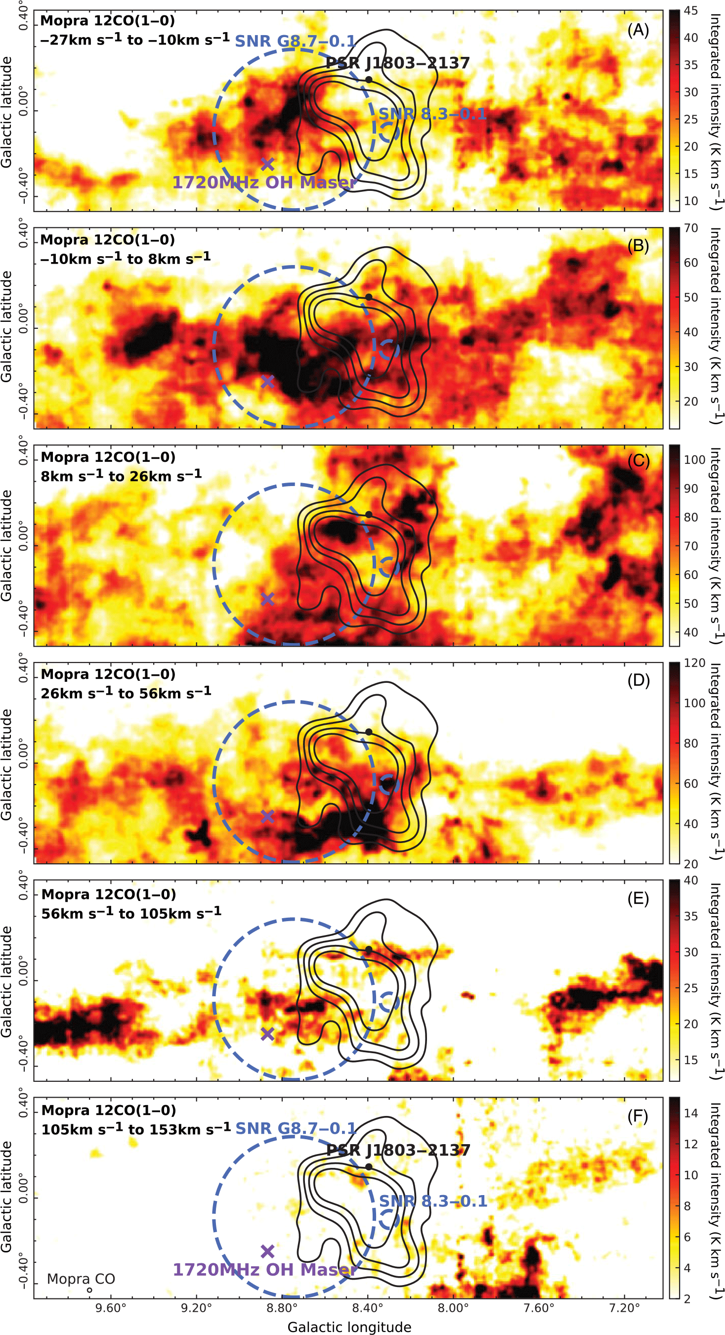
Mosaic of Mopra ${^{13}\text{CO}}$
integrated intensity maps (K
${^{13}\text{CO}}$
integrated intensity maps (K ${\,\,\text{km\,s}^{-1}}$
) towards
${\,\,\text{km\,s}^{-1}}$
) towards ${\text{HESS\,J}1804{-}216}$
. The two dashed blue circles indicate
${\text{HESS\,J}1804{-}216}$
. The two dashed blue circles indicate ${\text{SNR\,G}8.7{-}0.1}$
and
${\text{SNR\,G}8.7{-}0.1}$
and ${\text{SNR}\,8.3{-}0.1}$
. The 1720-MHz OH is indicated by the purple cross and
${\text{SNR}\,8.3{-}0.1}$
. The 1720-MHz OH is indicated by the purple cross and ${\text{PSR\,J}1803{-}2137}$
is indicated by the black dot. The TeV
${\text{PSR\,J}1803{-}2137}$
is indicated by the black dot. The TeV ${\gamma}$
-ray emission for 5-10
${\gamma}$
-ray emission for 5-10 ${\sigma}$
is shown by the solid black contours. The aqua circles in component D indicate Hii regions.
${\sigma}$
is shown by the solid black contours. The aqua circles in component D indicate Hii regions.

Mosaic of SGPS HI integrated intensity maps (K ${\,\,\text{km\,s}^{-1}}$
) towards
${\,\,\text{km\,s}^{-1}}$
) towards ${\text{HESS\,J}1804{-}216}$
. The two dashed blue circles indicate
${\text{HESS\,J}1804{-}216}$
. The two dashed blue circles indicate ${\text{SNR\,G}8.7{-}0.1}$
and
${\text{SNR\,G}8.7{-}0.1}$
and ${\text{SNR}\,8.3{-}0.1}$
. The 1720-MHz OH is indicated by the purple cross and
${\text{SNR}\,8.3{-}0.1}$
. The 1720-MHz OH is indicated by the purple cross and ${\text{PSR\,J}1803{-}2137}$
is indicated by the black dot. The TeV
${\text{PSR\,J}1803{-}2137}$
is indicated by the black dot. The TeV ${\gamma}$
-ray emission for 5-10
${\gamma}$
-ray emission for 5-10 ${\sigma}$
is shown by the solid black contours.
${\sigma}$
is shown by the solid black contours.
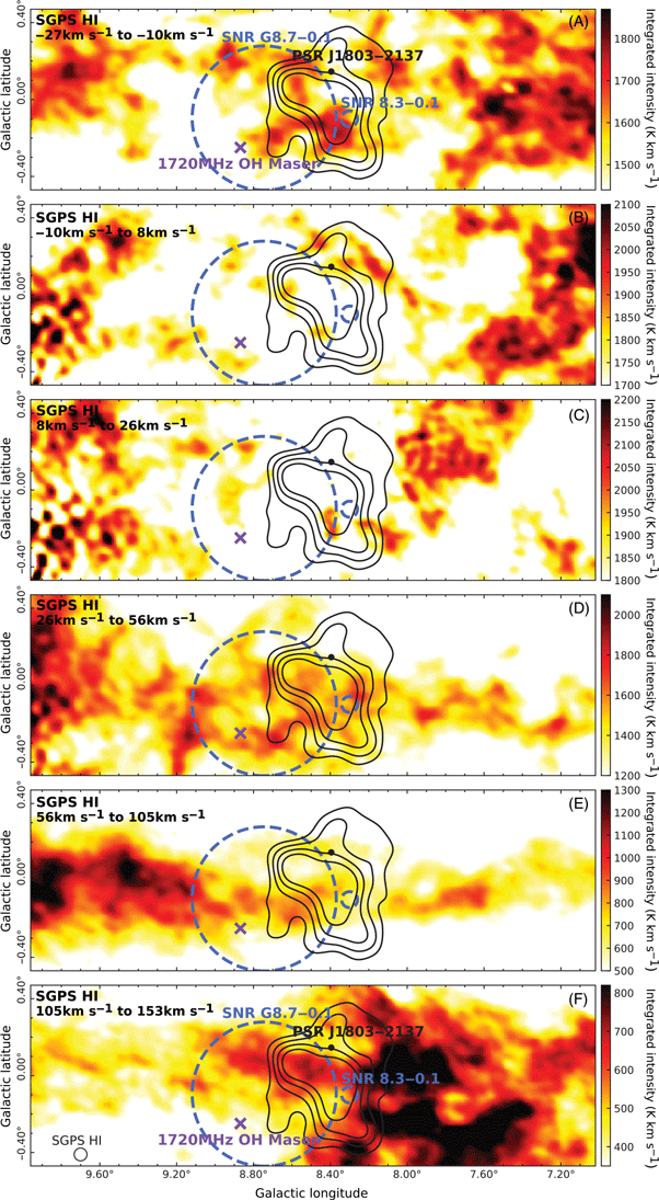
Total column density maps, ${2N_{\text{H}_{2}}+N_{\text{HI}}}$
, (
${2N_{\text{H}_{2}}+N_{\text{HI}}}$
, ( ${\text{cm}^{-2}}$
) towards
${\text{cm}^{-2}}$
) towards ${\text{HESS\,J}1804{-}216}$
, for gas components E and F. The two dashed blue circles indicate
${\text{HESS\,J}1804{-}216}$
, for gas components E and F. The two dashed blue circles indicate ${\text{SNR\,G}8.7{-}0.1}$
and
${\text{SNR\,G}8.7{-}0.1}$
and ${\text{SNR}\,8.3{-}0.1}$
. The 1720-MHz OH is indicated by the purple cross and
${\text{SNR}\,8.3{-}0.1}$
. The 1720-MHz OH is indicated by the purple cross and ${\text{PSR\,J}1803{-}2137}$
is indicated by the black dot. The TeV
${\text{PSR\,J}1803{-}2137}$
is indicated by the black dot. The TeV ${\gamma}$
-ray emission for 5-10
${\gamma}$
-ray emission for 5-10 ${\sigma}$
is shown by the solid black contours.
${\sigma}$
is shown by the solid black contours.

Ratio of molecular hydrogen ( ${N_{\text{H}_{2}}}$
) and atomic hydrogen (
${N_{\text{H}_{2}}}$
) and atomic hydrogen ( ${N_{\text{HI}}}$
) column densities towards
${N_{\text{HI}}}$
) column densities towards ${\text{HESS\,J}1804{-}216}$
, for gas components A–E. The two dashed blue circles indicate
${\text{HESS\,J}1804{-}216}$
, for gas components A–E. The two dashed blue circles indicate ${\text{SNR\,G}8.7{-}0.1}$
and
${\text{SNR\,G}8.7{-}0.1}$
and ${\text{SNR}\,8.3{-}0.1}$
. The 1720-MHz OH is indicated by the purple cross and
${\text{SNR}\,8.3{-}0.1}$
. The 1720-MHz OH is indicated by the purple cross and ${\text{PSR\,J}1803{-}2137}$
is indicated by the black dot. The TeV
${\text{PSR\,J}1803{-}2137}$
is indicated by the black dot. The TeV ${\gamma}$
-ray emission for 5-10
${\gamma}$
-ray emission for 5-10 ${\sigma}$
is shown by the solid black contours.
${\sigma}$
is shown by the solid black contours.

Top: Total column density map ( ${\text{cm}^{-2}}$
) from the SGPS HI and Mopra
${\text{cm}^{-2}}$
) from the SGPS HI and Mopra ${^{12}\text{CO}}$
emission, along the entire line of sight (
${^{12}\text{CO}}$
emission, along the entire line of sight ( ${\text{v}_{\text{lsr}}=50}$
to
${\text{v}_{\text{lsr}}=50}$
to ${150\,\,\text{km\,s}^{-1}}$
) of
${150\,\,\text{km\,s}^{-1}}$
) of ${\text{HESS\,J}1804{-}216}$
. Middle: Planck hydrogen column density. Bottom: Ratio of hydrogen column density as derived from Planck dust opacity and Hii column density from free–free emission. All: The two dashed blue circles indicate
${\text{HESS\,J}1804{-}216}$
. Middle: Planck hydrogen column density. Bottom: Ratio of hydrogen column density as derived from Planck dust opacity and Hii column density from free–free emission. All: The two dashed blue circles indicate ${\text{SNR\,G}8.7{-}0.1}$
and
${\text{SNR\,G}8.7{-}0.1}$
and ${\text{SNR}\,8.3{-}0.1}$
. The 1720-MHz OH is indicated by the purple cross and
${\text{SNR}\,8.3{-}0.1}$
. The 1720-MHz OH is indicated by the purple cross and ${\text{PSR\,J}1803{-}2137}$
is indicated by the black dot. The TeV
${\text{PSR\,J}1803{-}2137}$
is indicated by the black dot. The TeV ${\gamma}$
-ray emission for 5-10
${\gamma}$
-ray emission for 5-10 ${\sigma}$
is shown by the solid black contours.
${\sigma}$
is shown by the solid black contours.

CS(1-0) integrated intensity maps ( ${\text{K\,km\,s}^{-1}}$
) towards
${\text{K\,km\,s}^{-1}}$
) towards ${\text{HESS\,J}1804{-}216}$
. For components A through F, the
${\text{HESS\,J}1804{-}216}$
. For components A through F, the ${\text{T}_{\text{rms}}}$
is 2.5, 2.7, 2.8, 3.5, 4.3, and 4.2 K, respectively. The two dashed blue circles indicate
${\text{T}_{\text{rms}}}$
is 2.5, 2.7, 2.8, 3.5, 4.3, and 4.2 K, respectively. The two dashed blue circles indicate ${\text{SNR\,G}8.7{-}0.1}$
and
${\text{SNR\,G}8.7{-}0.1}$
and ${\text{SNR}\,8.3{-}0.1}$
. The 1720-MHz OH is indicated by the purple cross and
${\text{SNR}\,8.3{-}0.1}$
. The 1720-MHz OH is indicated by the purple cross and ${\text{PSR\,J}1803{-}2137}$
is indicated by the black dot. The TeV
${\text{PSR\,J}1803{-}2137}$
is indicated by the black dot. The TeV ${\gamma}$
-ray emission for 5-10
${\gamma}$
-ray emission for 5-10 ${\sigma}$
is shown by the solid black contours.
${\sigma}$
is shown by the solid black contours.

SiO(1-0, v = 0) integrated intensity maps ( ${\text{K\,km\,s}^{-1}}$
) towards
${\text{K\,km\,s}^{-1}}$
) towards ${\text{HESS\,J}1804{-}216}$
. For components A through F, the
${\text{HESS\,J}1804{-}216}$
. For components A through F, the ${\text{T}_{\text{rms}}}$
is 1.3 K, 1.3 K, 1.4 K, 1.7 K, 2.2 K, and 2.2 K, respectively. The two dashed blue circles indicate
${\text{T}_{\text{rms}}}$
is 1.3 K, 1.3 K, 1.4 K, 1.7 K, 2.2 K, and 2.2 K, respectively. The two dashed blue circles indicate ${\text{SNR\,G}8.7{-}0.1}$
and
${\text{SNR\,G}8.7{-}0.1}$
and ${\text{SNR}\,8.3{-}0.1}$
. The 1720-MHz OH is indicated by the purple cross and
${\text{SNR}\,8.3{-}0.1}$
. The 1720-MHz OH is indicated by the purple cross and ${\text{PSR\,J}1803{-}2137}$
is indicated by the black dot. The TeV
${\text{PSR\,J}1803{-}2137}$
is indicated by the black dot. The TeV ${\gamma}$
-ray emission for 5-10
${\gamma}$
-ray emission for 5-10 ${\sigma}$
is shown by the solid black contours.
${\sigma}$
is shown by the solid black contours.
 ${\text{HC}_3}$
N(5-4) integrated intensity maps (
${\text{HC}_3}$
N(5-4) integrated intensity maps ( ${\text{K\,km\,s}^{-1}}$
) towards
${\text{K\,km\,s}^{-1}}$
) towards ${\text{HESS\,J}1804{-}216}$
. For components A through F, the
${\text{HESS\,J}1804{-}216}$
. For components A through F, the ${\text{T}_{\text{rms}}}$
is 3.6 K, 3.8 K, 3.8 K, 4.9 K, 6.1 K, and 6.1 K, respectively. The two dashed blue circles indicate
${\text{T}_{\text{rms}}}$
is 3.6 K, 3.8 K, 3.8 K, 4.9 K, 6.1 K, and 6.1 K, respectively. The two dashed blue circles indicate ${\text{SNR\,G}8.7-0.1}$
and
${\text{SNR\,G}8.7-0.1}$
and ${\text{SNR}\,8.3{-}0.1}$
. The 1720-MHz OH is indicated by the purple cross and
${\text{SNR}\,8.3{-}0.1}$
. The 1720-MHz OH is indicated by the purple cross and ${\text{PSR\,J}1803{-}2137}$
is indicated by the black dot. The TeV
${\text{PSR\,J}1803{-}2137}$
is indicated by the black dot. The TeV ${\gamma}$
-ray emission for 5-10
${\gamma}$
-ray emission for 5-10 ${\sigma}$
is shown by the solid black contours.
${\sigma}$
is shown by the solid black contours.
 ${\text{CH}_3}$
OH integrated intensity maps (
${\text{CH}_3}$
OH integrated intensity maps ( ${\text{K\,km\,s}^{-1}}$
, uncleaned) towards
${\text{K\,km\,s}^{-1}}$
, uncleaned) towards ${\text{HESS\,J}1804{-}216}$
. For components A through F, the
${\text{HESS\,J}1804{-}216}$
. For components A through F, the ${\text{T}_{\text{rms}}}$
is 0.8 K, 0.9 K, 0.9 K, 1.1 K, 1.4 K, and 1.4 K, respectively. The two dashed blue circles indicate
${\text{T}_{\text{rms}}}$
is 0.8 K, 0.9 K, 0.9 K, 1.1 K, 1.4 K, and 1.4 K, respectively. The two dashed blue circles indicate ${\text{SNR\,G}8.7{-}0.1}$
and
${\text{SNR\,G}8.7{-}0.1}$
and ${\text{SNR}\,8.3{-}0.1}$
. The 1720-MHz OH is indicated by the purple cross and
${\text{SNR}\,8.3{-}0.1}$
. The 1720-MHz OH is indicated by the purple cross and ${\text{PSR\,J}1803{-}2137}$
is indicated by the black dot. The TeV
${\text{PSR\,J}1803{-}2137}$
is indicated by the black dot. The TeV ${\gamma}$
-ray emission for 5-10
${\gamma}$
-ray emission for 5-10 ${\sigma}$
is shown by the solid black contours.
${\sigma}$
is shown by the solid black contours.
 ${\text{NH}_3(1,1)}$
integrated intensity maps (
${\text{NH}_3(1,1)}$
integrated intensity maps ( ${\text{K\,km\,s}^{-1}}$
) towards
${\text{K\,km\,s}^{-1}}$
) towards ${\text{HESS\,J}1804{-}216}$
using HOPS data. The two dashed blue circles indicate
${\text{HESS\,J}1804{-}216}$
using HOPS data. The two dashed blue circles indicate ${\text{SNR\,G}8.7{-}0.1}$
and
${\text{SNR\,G}8.7{-}0.1}$
and ${\text{SNR}\,8.3{-}0.1}$
. The 1720-MHz OH is indicated by the purple cross and
${\text{SNR}\,8.3{-}0.1}$
. The 1720-MHz OH is indicated by the purple cross and ${\text{PSR\,J}1803{-}2137}$
is indicated by the black dot. The TeV
${\text{PSR\,J}1803{-}2137}$
is indicated by the black dot. The TeV ${\gamma}$
-ray emission for 5-10
${\gamma}$
-ray emission for 5-10 ${\sigma}$
is shown by the solid black contours.
${\sigma}$
is shown by the solid black contours. ${\text{H}_2\text{O}}$
maser positions are shown by the green dots.
${\text{H}_2\text{O}}$
maser positions are shown by the green dots.

Modelled energy spectra of CR protons (Equation (14)) escaping from the potential impulsive accelerator ${\text{SNR\,G}8.7{-}0.1}$
, with a total energy of
${\text{SNR\,G}8.7{-}0.1}$
, with a total energy of ${{2\times10^{48}}}$
erg in CRs. Various values of diffusion suppression factor,
${{2\times10^{48}}}$
erg in CRs. Various values of diffusion suppression factor, ${\chi}$
, and index of the diffusion coefficient,
${\chi}$
, and index of the diffusion coefficient, ${\delta}$
, are shown here. A power law spectrum with a spectral index of
${\delta}$
, are shown here. A power law spectrum with a spectral index of ${{\alpha}=2}$
is assumed. The number density is taken to be
${{\alpha}=2}$
is assumed. The number density is taken to be ${n=160\,\text{cm}^{-3}}$
. The distance from the accelerator to the cloud is
${n=160\,\text{cm}^{-3}}$
. The distance from the accelerator to the cloud is ${R\mathord{\sim}12\,\text{pc}}$
and age of the source are taken to be 15 kyr and 28 kyr for the cyan and black curves, respectively. The magenta dashed line represents the CR flux observed at Earth. The red represents the calculated CR enhancement factor for
${R\mathord{\sim}12\,\text{pc}}$
and age of the source are taken to be 15 kyr and 28 kyr for the cyan and black curves, respectively. The magenta dashed line represents the CR flux observed at Earth. The red represents the calculated CR enhancement factor for ${\text{HESS\,J}1804{-}216}$
(
${\text{HESS\,J}1804{-}216}$
( ${k_{\rm CR}\approx37}$
). The green represents the calculated CR enhancement factor for
${k_{\rm CR}\approx37}$
). The green represents the calculated CR enhancement factor for ${\text{FGES\,J}1804.8{-}2144}$
(
${\text{FGES\,J}1804.8{-}2144}$
( ${k_{\rm CR}\approx9}$
).
${k_{\rm CR}\approx9}$
).

Modelled energy spectra of CR protons (Equation (14)) escaping from the potential impulsive accelerator (progenitor SNR from ${\text{PSR\,J}1803{-}2137}$
), with a total energy of
${\text{PSR\,J}1803{-}2137}$
), with a total energy of ${{10}^{{48}}}$
erg in CRs. Various values of diffusion suppression factor,
${{10}^{{48}}}$
erg in CRs. Various values of diffusion suppression factor, ${\chi}$
, and index of the diffusion coefficient,
${\chi}$
, and index of the diffusion coefficient, ${\delta}$
, are shown here. A power law spectrum with a spectral index of
${\delta}$
, are shown here. A power law spectrum with a spectral index of ${{{\alpha}}=2}$
is assumed. The number density is taken to be
${{{\alpha}}=2}$
is assumed. The number density is taken to be ${n=325\,\text{cm}^{-3}}$
. The distance from the accelerator to the cloud is
${n=325\,\text{cm}^{-3}}$
. The distance from the accelerator to the cloud is ${R\mathord{\sim}10\,\text{pc}}$
and age of the source is taken to be 16 kyr for the black curves. The magenta dashed line represents the CR flux observed at Earth. The red represents the calculated CR enhancement factor for
${R\mathord{\sim}10\,\text{pc}}$
and age of the source is taken to be 16 kyr for the black curves. The magenta dashed line represents the CR flux observed at Earth. The red represents the calculated CR enhancement factor for ${\text{HESS\,J}1804{-}216}$
(
${\text{HESS\,J}1804{-}216}$
( ${k_{\rm CR}\approx57}$
). The green represents the calculated CR enhancement factor for
${k_{\rm CR}\approx57}$
). The green represents the calculated CR enhancement factor for ${\text{FGES\,J}1804.8{-}2144}$
(
${\text{FGES\,J}1804.8{-}2144}$
( ${k_{\rm CR}\approx14}$
).
${k_{\rm CR}\approx14}$
).


